Article

Water Quality Grade Identification for Lakes in Middle Reaches of Yangtze River Using Landsat-8 Data with Deep Neural Networks (DNN) Model

1
Faculty of Resources and Environmental Science, Hubei University, Wuhan 430062, China
2
Hubei Key Laboratory of Regional Development and Environmental Response, Hubei University, Wuhan 430062, China
3
Key Laboratory of Natural Resources Monitoring and Supervision in Southern Hilly Region, Ministry of Natural Resources, Changsha 410118, China
4
Department of Geography and Environmental Science, University of Reading, Reading RG6 6AB, UK
5
State Key Laboratory of Hydrology-Water Resources and Hydraulic Engineering, Hohai University, Nanjing 210098, China
6
Hubei Spatial Planning Research Institute, Wuhan 430061, China
*
Author to whom correspondence should be addressed.
Remote Sens. 2022, 14(24), 6238; https://doi.org/10.3390/rs14246238
Submission received: 13 October 2022 / Revised: 25 November 2022 / Accepted: 7 December 2022 / Published: 9 December 2022

Abstract

:
Water quality grade is an intuitive element for people to understand the condition of water quality. However, in situ water quality grade measurements are often labor intensive, which makes measurement over large areas very costly and laborious. In recent years, numerous studies have demonstrated the effectiveness of remote sensing techniques in monitoring water quality. In order to automatically extract the water quality information, machine learning technologies have been widely applied in remote sensing data interoperation. In this study, Landsat-8 data and deep neural networks (DNN) were employed to identify the water quality grades of lakes in two cities, Wuhan and Huangshi, in the middle reach of the Yangtze River, central China. Additionally, linear support vector machine (L-SVM), random forest (RF), decision tree (DT), and multi-layer perceptron (MLP) were selected as comparative methods. The experimental results showed that DNN achieved the most promising performance compared to the other approaches. For the lakes in Wuhan, DNN gave water quality results with overall accuracy (OA) of 93.37% and Kappa of 0.9028. For the lakes in Huangshi, OA and kappa given by DNN were 96.39% and 0.951, respectively. The results show that the use of remote sensing images for water quality grade monitoring is effective. In the future, our method can be used for water quality monitoring of lakes in large areas at a low cost.

1. Introduction

With the acceleration of urbanization and industrialization, water pollution has become a major challenge for the sustainable development of the country [1,2]. Therefore, water quality monitoring techniques have drawn the attention of the government and research institutions. The traditional water quality survey method depends on the on-site sample collection, which is inevitably labor-intensive and costly [3,4]. Thanks to the rapid development of optical remote sensing technology, it has been utilized in large-scale dynamic water quality identification, owing to its advantages of wide monitoring range, fast speed, and low cost [5]. The Landsat 8 OLI, for example, provides relatively fine spatial (30 m) and spectral resolution data, containing 11 bands, with a wavelength range from 0.43 nm to 1.38 nm. Rich spectral information makes wide use of Landsat 8 OLI images in monitoring a variety of water quality parameters.
The optical remote sensing imagery records the spectral information of water, where the polluted water and clean water show different characteristics at specific wavelengths [6,7]. Therefore, the remote sensing and ground monitoring data were fused for the quantitative inversion of colored substances in water, and the strong optically active water-colored substances had been extensively studied [8]. The traditional methods include an empirical method and a semi-analytical method. Although no physical, chemical or other assumptions are made, these methods can still establish a mathematical relationship between water quality parameters and spectral information. For example, onboard the Suomi National Polar-orbiting Partnership (SNPP) satellite, Son et al. [9] were able to retrieve chlorophyll a (Chla) in the Great Lakes by utilizing the maximum ratio of normalized water-leaving radiance at the blue and green bands. Based on in-situ measurements and synchronous MODIS imagery, Wang et al. [10] developed and validated a Forel-Ule Index (FUI) and hue angle-based model to estimate Secchi disk depth (ZSD) for large lakes across China.
In addition, new methods such as artificial intelligence algorithms are popularized in the field of remote sensing, which also provides a new train of thought for water quality monitoring. Kupssinskü et al. [11] estimated the total suspended solids (TSS) and Chla concentration by combining laboratory analysis data with different spatial resolution data from Sentinel-2 spectral images and unmanned aerial vehicles. In response to the inverse problem of retrieving Chla from reflectance for the Sentinel-2 (MSI) and Sentinel-3 (OLCI) observatories, Pahlevan et al. [12] propose a novel machine-learning algorithm (MDN). In addition, to obtain the Chla concentrations of the Yangtze River Plain lakes, Guan et al. [13] combined OLCI images and an integrated SVR-based algorithm for accurate retrieval. It is not difficult to find that these water quality monitoring studies generally only focus on one or a few strong optically active substances [14,15]. Ordinary machine learning algorithms have a simpler structure and limited ability to solve complex problems. Deep learning models represented by DNN have been increasingly used to deal with exploratory problems in the earth domain due to their ability to automatically extract features and handle high-dimensional data.
After several decades of rapid economic development, China has paid more attention to managing water resources, including preventing and controlling water pollution, protecting surface water quality, safeguarding people’s health, and maintaining ecological safety. In particular, the middle reach of the Yangtze River basin has a large number of lakes and a dense network of rivers. At the same time, the surrounding industries and urbanization are progressing rapidly. This has put enormous pressure on the ecology of the lake waters. Water quality monitoring is particularly necessary. The study of water quality conditions of lakes not only promotes the function of river and lake systems and water safety but also has important implications for future hydrological prediction and artificial intervention efforts in the region.
National Environmental Protection Agency has released Environmental Quality Standards for Surface Water (GB 3838-2002, http://sthjt.hubei.gov.cn/ (accessed on 15 October 2019)) [16]. According to the above standards and the water quality automatic monitoring report issued by the China National Environmental Monitoring Centre, the water grade of surface waters is quantified into six grades (I, II, III, IV, V, and VI) [17]. Grades I and II water can be used as a source of drinking water for residents after certain treatments. Grade III water is mainly used for aquaculture as well as swimming. Grade IV water is used for the industrial sector. Grade V water can only be used for agricultural irrigation and general landscape water. Any water that is contaminated beyond the standard of Grade V is classified as Grade VI water.
According to China’s requirements for surface water monitoring, water quality must be measured once every two months. Each water grade is evaluated by testing 24 indicators. The basic water quality parameters include total phosphorus (TP), total nitrogen (TN), biochemical oxygen demand (BOD5), chemical oxygen demand (COD), permanganate index (CODMN), ammonia nitrogen (NH3-N), and heavy metals. The grade identified by the worst indicator is used as the grade for the water body. Therefore, the traditional method for identifying the water quality grade requires measuring a large number of indicators in a certain period. This is costly, cumbersome, and inefficient [18,19].
In this context, this study applied Landsat 8 satellite image as the data source to classify the water quality grades for the lakes in the middle reaches of the Yangtze River, Central China. Meanwhile, to extract water quality grades from the remote sensing data, several machine learning models are leveraged and compared (DT, L-SVM, MLP, and RF). Therefore, the main objectives of the study are to (1) explore the potential of the DNN model for large-scale water quality grade recognition, and (2) use remote sensing images to classify the water quality grade of lakes and reduce the reliance on water quality parameters.

2. Materials and Methods

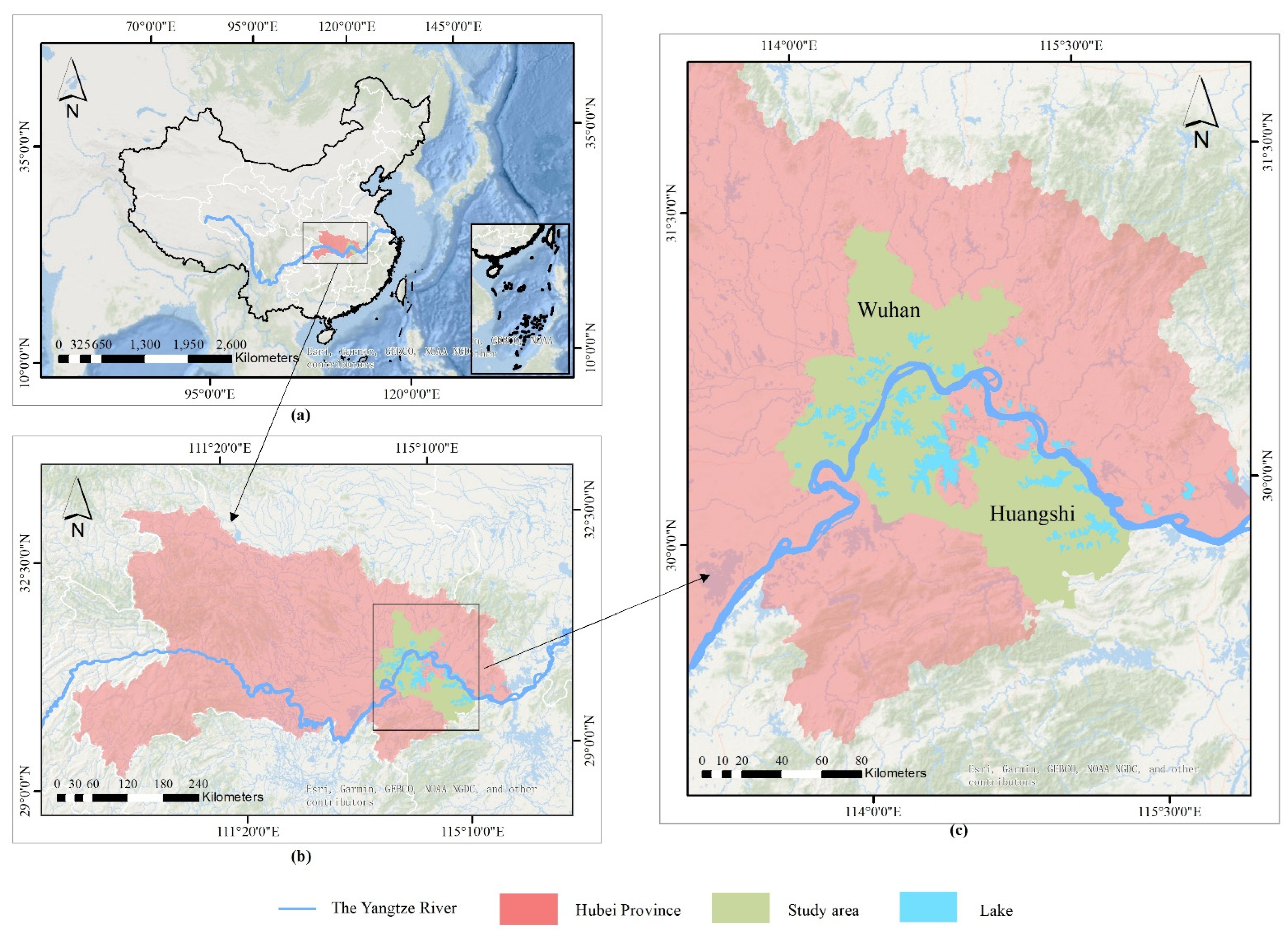
2.1. Study Areas and Datasets

2.1.1. Study Areas

Lakes in Wuhan, Huangshi, and their surrounding areas in the middle reaches of the Yangtze River are used as research areas (Figure 1b). Wuhan City is crossed by the Yangtze River and is divided into two parts. Water covers a quarter of the city’s total area, with an area of 803.17 km2. It is rich in fresh water and has a large proportion of surface water in the city in China [20,21]. Its per capita water resources are about 40 times the national average. This research selected 76 lakes in Wuhan City as the first research area (Wuhan dataset) (Figure 1c). The northeast part of Huangshi City is close to the Yangtze River. Similar to Wuhan, Huangshi City is rich in surface water resources. A total of 49 lakes in Huangshi City and its surrounding areas were chosen to be another study area (Figure 1c). The central part of the Yangtze River basin is among the areas with the highest population density, the highest intensity of economic activities, and the most serious environmental pressure in China. The problem of eutrophication in water bodies is becoming worse every year, and the water ecological environment is facing a great challenge [22]. Applying remote sensing methods to identify water quality grades and monitor water quality changes regularly can provide a good foundation for the government to make effective measures to control water pollution in the region.

2.1.2. Image Data

The Landsat 8 OLI images (7 bands) selected for this experiment were obtained from the United States Geological Survey (USGS) (https://www.usgs.gov/ (accessed on 15 October 2019)). The Landsat 8 satellite was launched in 2013 and carries two sensors, the Operational Land Imager (OLI) and the Thermal Infrared Sensor (TIRS). The satellite has a total of 11 bands, divided into bands 1–7 (coastal, blue, green, red, near-infrared, and two short-wave infrared bands), and 9–11 (cirrus and two thermal infrared bands) with a spatial resolution of 30 m and band 8 having a panchromatic resolution of 15 m. The satellite can achieve global coverage once every 16 days.
In this study, two images were selected. The image for the Wuhan study area was taken in April 2018, and the imaging for the Huangshi study area was taken in April 2017. The data type of both images was L1T, and a total of seven bands (1–7) were selected with a spatial resolution of 30 m. In order to ensure no weather influence, the selected images were free of cloud coverage.

2.1.3. Water Quality and Water Vector Data

The water quality data of the two study areas are from the Wuhan Bureau of Ecology and Environment (http://hbj.wuhan.gov.cn (accessed on 15 October 2019)) and Hubei Province Environmental Monitoring Center Station (http://sthjt.hubei.gov.cn (accessed on 15 October 2019)), respectively. According to the HJ/T 91-2002 document, the frequency of water quality surveys is generally once every two months. Combined with the continuous water quality assessment report provided by the Chinese Environmental Monitoring Department, it was found that the water quality grades of inland lakes did not change much in the short term [23]. Several representative lakes are listed in Table 1. They have several parameters that exceed the standard values and the values inside the brackets are the standard value of the grade of water quality.

2.2. Methods

2.2.1. Deep Neural Networks

There are two parts to the Deep Neural Networks (DNN) training process, those being the signal’s forward propagation and the error’s reverse propagation [24,25]. Backpropagation is the core of training neural networks. It can reduce the model’s loss value by optimizing the neural network’s weight and bias under the defined loss function. In our work, the deployment of DNN models is mainly carried out through Python and TensorFlow.
The DNN is initialized before training, and the network initialization is very important for finding globally optimal results [26]. Inappropriate weight initialization makes the derivative close to zero when passing through the activation function, so the premature gradient disappears. This study used the Xavier initializer, which automatically adjusts the most appropriate distribution based on the number of input and output nodes in the network layer [27]. Its distribution satisfies:
W ~ U [ 6 / ( n i n + n o u t ) , 6 / ( n i n + n o u t ) ]
where n i n and n o u t   are the input dimension and the output dimension [28].
In general, the linear rectifier function refers to the ramp function in mathematics, which can be written as:
a r e l u ( x ) = max ( 0 , x )
Furthermore, in the middle of the neural network, a rectified linear unit (ReLU) is used as the activation function of the neuron, which defines the nonlinear output of the neuron after linear transformation. For the input vector from the previous layer of the neural network entering the neuron, the neuron using the linear rectification activation function will output:
z ( x ) = w T x + b
The ReLU can effectively limit the gradient explosion or gradient disappearance and simplifies the calculation process. As a result, it is a commonly used activation function in neural networks.
Softmax is a logistic regression algorithm that aims to present the results of multiple classifications in the form of probabilities, which are added to the last layer [29]. The probability distributions of the water quality grades predicted by a single pixel on the entire image are finally obtained, and the one with the highest proportion is considered the prediction result. The cross-entropy function was selected:
L = y i ln a i
where a(x) is the output of the softmax, and y is the true value of the water quality grade corresponding to the pixel.
The deep network is called the MLP model if it only comprises of the above process. However, the excellent predictive ability of deep learning depends more on the optimization process of back-propagation, which is a process of continuously calculating the gradients and adjusting the learnable parameters. The parameters are the weight w and the offset b in the linear function z(x). The updated formula for w and b is [30]:
w [ l ] = w [ l ] α d w [ l ]
b [ l ] = b [ l ] α d b [ l ]
where α is the learning rate. Superscript l indicates the l-th hidden layer of the neural network. d w and d b indicate that the cross-entropy loss function L(x) seeks the partial derivatives for the weights and offsets. When the learning rate is too large, the loss value can easily fluctuate or even explode at the lowest point. When the learning rate is too small, it will slow down the whole training process or the model will be overfitted.
The effectiveness of the neural network in expressing a model is largely related to the optimization algorithm. Stochastic gradient descent (SGD), momentum, the adaptive gradient (Adagrad), and root mean square prop (RMSProp) are commonly used optimizers [31,32,33,34]. Kingma and Ba [35] proposed the adaptive moment estimation (Adam) optimizer to consider the update step size for the current moment estimation and the next moment estimation of the gradient. Adam optimizer combines the advantages of both Adagrad and RMSProp. Its high computational efficiency is more advantageous when applied to large-scale data. The parameter update is also not affected by the gradient transformation. Therefore, we choose Adam as the optimization algorithm for the DNN model in this experiment.
In addition, since the number of dataset samples used in this study reached tens of thousands, it was slower to train the entire dataset at the same time. The mini-batch method can solve the discrete value problem of categorical data and is more reasonable in the distance calculation problem of the loss function. Due to the small number of water quality grades, the mini-batch method was suitable for encoding the water quality grades using one-hot encoding [36]. Therefore, we used the mini-batch method [37] to train the samples in batches.

2.2.2. Compared Models

In addition to the DNN model, this study also compares four other classical algorithms, all of which have been widely used in classification tasks for various scenarios.

Linear Support Vector Machine (L-SVM)

L-SVM is a kernel-based algorithm, and its basic idea is to solve the separated hyperplane that correctly partitions the training dataset and maximizes the geometric separation. It can achieve good results for classification tasks of the small sample [38,39,40].

Decision Tree (DT)

DT algorithm is built based on a given training dataset, so it can correctly classify instances, essentially generalizing a set of classification rules from the training set. It can produce feasible and effective results for a large dataset in a relatively short period [41,42].

Random Forest (RF)

RF is an algorithm that integrates multiple trees through the idea of integrating learning. It is composed of many decision trees, with no association between different decision trees. When performing a classification task, new input samples are entered and each decision tree in the forest is allowed to judge and classify them separately, and each decision tree will produce its classification result [43,44].

Multi-Layer Perceptron (MLP)

MLP is a classical artificial neural network model, which generally consists of an input layer, a hidden layer, and an output layer. The input layer is used to obtain the feature vectors of the dataset, and each feature vector is multiplied by its corresponding weight plus bias to form the hidden layer neurons. The output is obtained by multiplying all the neuron outputs of the last hidden layer by their weights and adding bias [45,46].

2.2.3. Training Data Preparation

Before making the dataset, the original image needs to be masked using a water vector in order to ensure that the experimental area is all water and does not contain any other ground objects. Geospatial Data Cloud (http://www.gscloud.cn/search (accessed on 15 October 2019)) provides water vector data. According to the water vector data, the image sizes after masking in the two study areas are 2983 × 3075 pixels and 4294 × 5209 pixels, respectively. The specific steps are as follows.
Firstly, the water vector data and remote sensing images were used for sample annotation to give the water quality grade of the lakes in the study area. Figure 2a,c show the Landsat 8 OLI images and the blue water vector, and the overlapped part is considered as the extent of the lakes. However, the water vector is only used as a reference, and the actual lake extent may be different from the water vector display. For example, in the red box marked in Figure 2a, the vector map shows that the area is a large river, but land accounts for the majority of the map. Moreover, in order to improve the accuracy of the experimental datasets, the regions of interest (ROIs) (Figure 2b,d) were selected by visual interpretation (grade II, light blue; grade III, green; grade IV, yellow; grade V, dark blue; grade VI, red) combined with the water vector from the Geospatial Data Cloud.
Secondly, the Landsat 8 OLI images were cropped based on the labeled ROIs to produce the final datasets [features, samples], where 10% of the data are used for training the model and the remaining 90% for testing. Since the random selection of training samples may lead to a change in classification results, the training dataset was randomly selected 10 times and the experiment was repeated. All image processing was carried out using ArcGIS 10.6 (ESRI, Redlands, CA, USA) and MATLAB software (Mathworks®, Natick, MA, USA).
After the water vector mask and before the ROI extraction, notably, the extraction of lakes was initially completed within the study area based on the water body index. However, some lakes existing in the water vector map may not be included in the datasets, which were made according to the ROIs depicted in Figure 2. The water quality grades in Table 2 correspond to Figure 2, and the last column shows the number of samples in all study areas. Combined with Figure 2, the sample sizes of each grade in Wuhan are unevenly distributed. The proportion of the inferior grade V waters is only 4%, grade II is 7%, and grade IV is the maximum, at 47%. The inconsistency between the ratio of the sample numbers of the dataset and the ratio of the lake numbers is due to the fragmentation of some lakes. For example, the grade VI lakes are concentrated around populated cities. These lakes are prone to eutrophication since they have poor circulation and self-cleaning capacity. For a very large grade IV Lake (Liangzi Lake), a large number of samples were also selected to ensure a uniform distribution of samples. For the lakes in the Huangshi, the proportions of water in each grade were close (20–30%). In addition, the division of the ROIs was based on the principle of uniform distribution, and the central area of the lake was selected as much as possible, in order to avoid the inconsistency of water quality between the shore and the lake center.

2.2.4. Accuracy Evaluation

According to the datasets produced, the five models of L-SVM, DT, RF, MLP, and DNN were trained. Based on the water maps, the final classification results for the two study areas were output. Kappa coefficient (Kappa) and the overall accuracy (OA) were used in classification problems to evaluate the prediction accuracy of the classifier, which was calculated by the confusion matrix. The confusion matrix can show the number and the grade of correct classification or misclassification of each ground object. However, the confusion matrix does not completely indicate classification accuracy. Therefore, it is essential to evaluate the classification result quantitatively by the index derived from the confusion matrix. OA represents the proportion of examples in the dataset that are correctly classified. Kappa is often used for multi-classification problems for consistency testing [47,48]. The higher the value, the stronger the consistency. In addition, the range of Kappa is usually [0, 1]. Kappa is calculated as follows [49]:
K a p p a = p o a p e 1 p e
p e = a 1 b 1 + a 2 b 2 + + a c b c n n
where p o a is the overall accuracy, a i is the number of target samples of the i-th grade, b i is the number of samples classified into the i-th grade, and n is the number of the entire sample.
The accuracy evaluation format was the difference between the mean deviation and the standard deviation of 10 experiments. The vector map of the water and the classification result map were superposed. The number of pixels for each water quality grade was calculated separately, and the grade with the highest percentage was considered to be the final water quality grade of the lake. The above evaluation process was implemented in Python.

3. Result

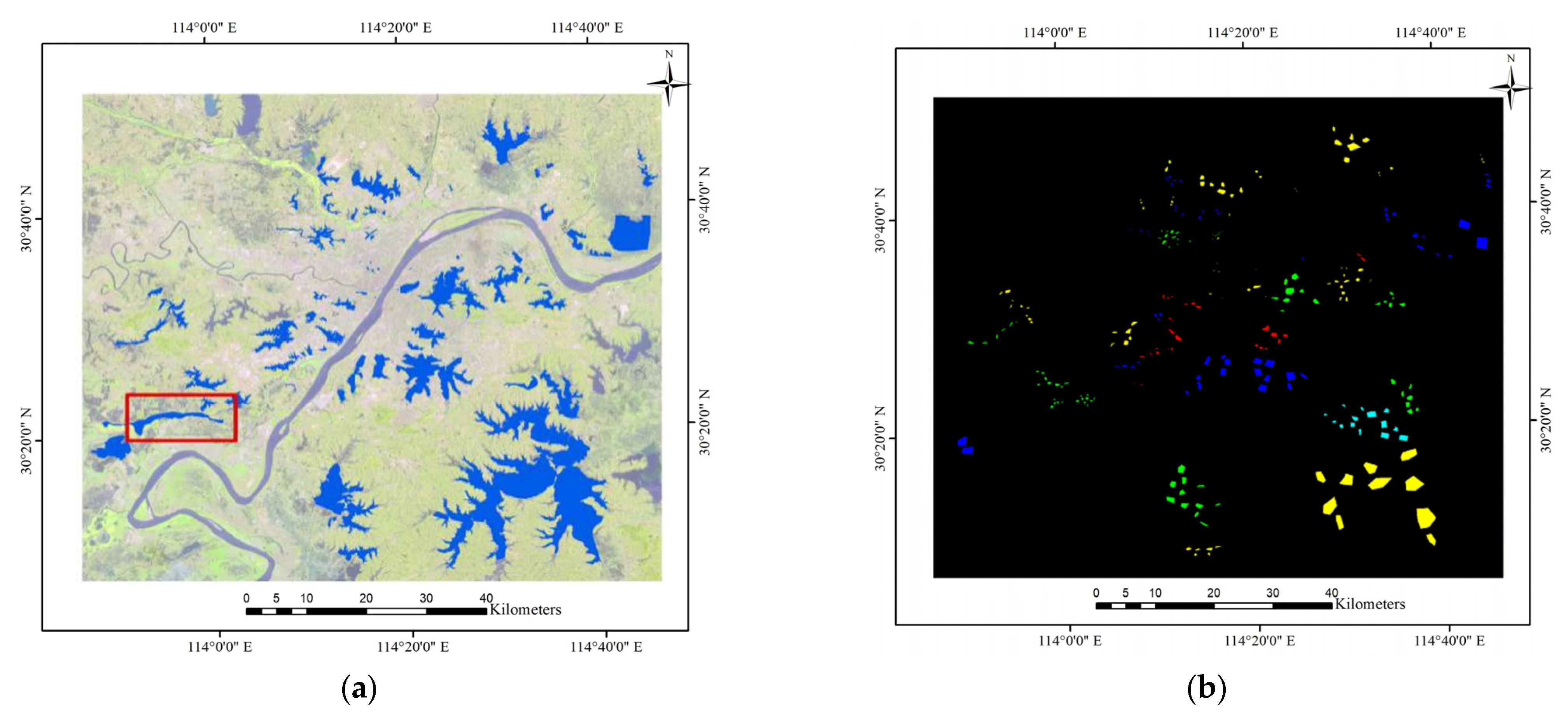
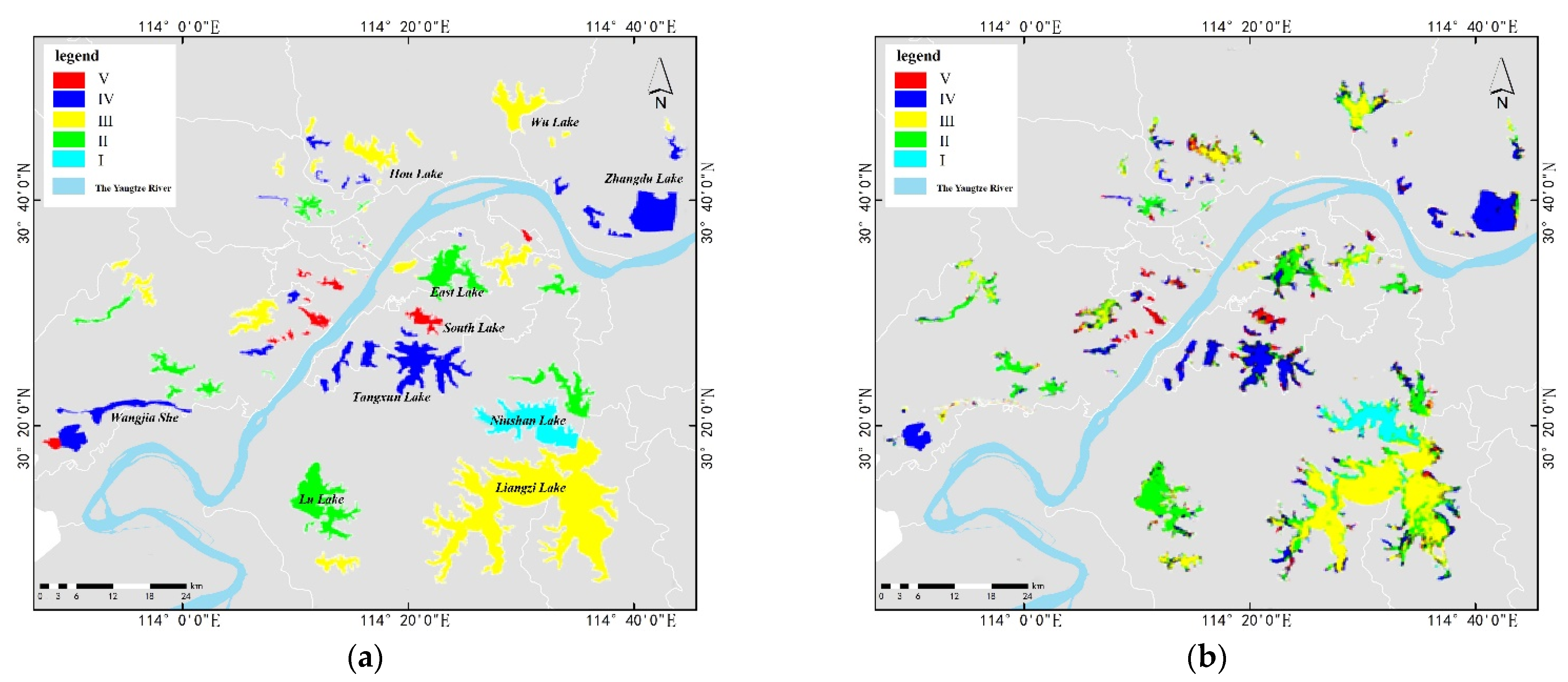
3.1. Experiment 1: The Wuhan Dataset

Experiment 1 targeted the water systems around Wuhan City. Table 3 shows the experimental accuracy of the Wuhan dataset. The supervised classification models were selected to explore the effects of the water quality classification, i.e., linear SVM (L-SVM), DT, RF, MLP, and DNN.
The hyperparameters of the model were determined by several experiments. For RF and DT, no adjustment of the maximum features is required due to the selection of 7 bands of Landsat 8 OLI images. In total, 100 trees were set in the experiment for RF. The minimum number of samples required to split an internal node was 10.
MLP was tuned in a similar way to DNN, where a maximum-minimum normalization is required before data input. When the depth and breadth of the network structure increased, the model accuracy did not improve and the parameters were fixed. The initial learning rate of MLP was set to 0.001, the maximum number of iterations was 1000, and the activation function was selected as ReLU.
The optimizer of DNN was chosen as Adam, with the highest accuracy and the most stability after several trials. Five hidden layers ( 2 8 ) were determined by manual adjustment of the neural network. According to the number of samples listed in Table 3, the minibatch was set to 2 11 . To avoid overfitting, the dropout method was used to randomly delete 10% of the neuron nodes, to make the models more adaptable and reduce the network complexity.
Table 3 compares the classification accuracy of all samples and individual labels for different classifiers. From the accuracy of each classifier for predicting the grade VI water grade, the prediction accuracy is significantly lower than for the other water quality grades. Furthermore, compared with the other grades, the standard deviation for grade V is the highest, indicating that the prediction result is unstable. This is the result of the lack of sufficient samples, which leads to poor predictive accuracy for this grade. The classification accuracies of the remaining four grades are the highest for the DNN model, reaching more than 90%. For the grade IV and grade V water grades, the predictive accuracy reaches more than 95%. Comparing all the classification results, the DNN model obtains the best prediction results, on average, and the Kappa of 0.9028 is 0.0186, higher than the result of RF. The standard deviation of the DNN prediction accuracy is the smallest, which indicates that the model has predictive stability. Although the DNN model uses the same deep structure as the MLP model, the classification accuracy of MLP is not as good without the backpropagation adjusting the weight and offset. The worst classification accuracy is obtained by L-SVM, for which the Kappa is 0.5229.
Based on the DNN model trained by the above methods, the water image extracted in step four was predicted. The spatial distribution of lake water quality grades in the Wuhan study area is shown in Figure 3a. The image on the left shows the true distribution. In general, most of the lakes can be accurately identified. Several different areas belonging to the same larger lake were classified into different grades. This is consistent with the fact that the lake water is not homogeneous, and the water quality is usually not consistent across the various areas of large lakes.
The figure shows that several major inferior-grade V lakes can be accurately predicted. However, the classification effect for a few lakes is not good. For example, South Lake is classified as both grade IV water and grade V water, which may be related to the uneven distribution of the lake water quality, and the noise in this part of the image may also have led to misclassification. From the overall classification results for all the lakes, the water quality grade of each lake can be easily determined. Niushan Lake (the only grade II lakes in the entire study area), Lu Lake and East Lake (grade III), Liangzi Lake, Hou Lake, and Wu Lake (grade IV), and Zhangdu Lake and Tangxun Lake (grade V) all show a clear classification of the water quality.
After completing the pixel-based classification task, the critical step is to establish statistics for the correct classification samples of each category for each lake. The result takes the maximum probability label to be the final grade of the lake. The statistics of the prediction results for the Wuhan dataset are shown in Table 4. Non-Water indicates that the lake has not been completely extracted by the modified normalized difference water index (MNDWI), and is not included in the counted category. As shown in Table 4, three lakes have not been extracted. The number of lakes that were correctly predicted is shown in bold. There was only one grade II Lake predicted correctly. Within the scope of the lakes, 78.45% of the samples were divided into grade II. The DNN model performs better in predicting grade III lakes, with all 13 lakes being predicted with 100% accuracy. Among the 29 grade IV lakes, 24 were accurately predicted for water quality. Moreover, two lakes were predicted to be grade III, and two lakes were predicted to be grade VI (inferior grade V). There are 20 lakes in grade V, except for one unextracted lake, the remaining 19 lakes were correctly identified. Ten of the 13 grade VI lakes were correctly predicted. However, one was still judged to be grade III, and one was judged to be grade V. According to the statistical results of all grade labels, 67 of the 73 lakes included in the statistics were correctly predicted, with a correct rate of 91.78%. Most of the lakes with incorrect predictions are small, considering the result is related to the number of samples and the presence of bottom reflection.

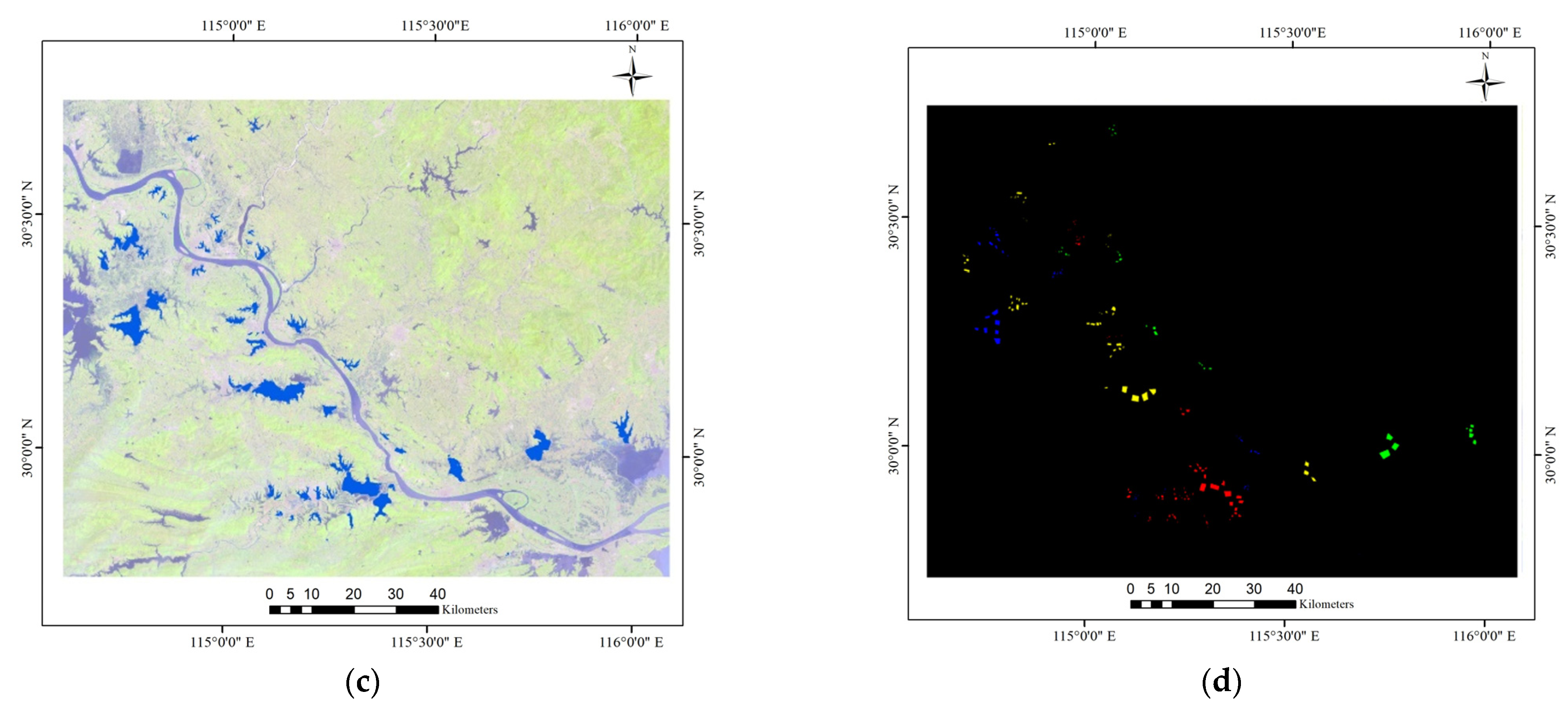
3.2. Experiment 2: The Huangshi Dataset

Another experiment targets the major lakes around Huangshi City, which are mostly on both sides of the Yangtze River. A comparison of different classification accuracy results is shown in Table 5. It should be noted that the parameter adjustment strategy for all classifiers is the same as in the previous experiment. In terms of classification results, L-SVM has the lowest classification accuracy among the five models. The prediction accuracies for the four grades of water quality are close, but the classification results are not ideal.
For DNN, the number of hidden layers is five ( 2 8 ). As in the Wuhan dataset, the Adam optimizer was selected with the following settings: a learning rate of 0.0001 and a number of iterations of 3000, and 10% of the neurons were randomly removed. Since the sample number of the Huangshi dataset is slightly less than that of the first dataset, the number of a batch was adjusted 2 10 . As shown in Table 5, the DNN model has the best prediction and higher accuracy than other models, and the Kappa is 0.0091 greater than that of RF. The Kappa is also 0.0482 higher than for the Wuhan dataset. There is no obvious grade with a high misclassification ratio, and the samples for the four grades have a prediction accuracy of 97.6%. The standard deviations of the average OA and Kappa are 0.17% and 0.0023, respectively. The results of several experiments show that the classification accuracy does not very much, and random changes in the training data do not have a large impact.
Figure 4a,c show the distribution maps generated from the water quality data provided in the government documents, and Figure 4b,d are the results predicted by the DNN model. Figure 4a,c are two parts of the same study area, with part c located downstream from part a. The two largest lakes in the grade V water quality grade are Baoan Lake and Wusi Lake. It is clear that the central areas of the lakes are all dark blue, but the shore areas are red or yellow. This suggests that the water quality of the lakes has been accurately determined, but the pollution degree may be significantly increased close to the bank and in the narrow channels, leading to the classification of the single sample as other grades. Other small lakes (dark blue) are classified into the grade V water quality grade. The largest grade VI lake in the study area is Wang Lake. Wang Lake and its surrounding grade VI lakes are classified accurately, Taibai Lake and Dayuan Lake in the lower reaches of the Yangtze River, as well as Ce Lake in the upper reaches, can be identified as grade III lakes.
Through the prediction results of the DNN model, the water quality grade of each lake can be determined. In particular, Wang Lake, Dazhi Lake, and the other large lakes which have relatively uniform water quality distributions are easily determined. However, for some lakes with a small area, such as Muyang Lake and Taihu Lake, the circulation of the lakes is poor, the degree of pollution varies greatly in different areas of the same lake, and the water quality is easily disturbed by natural and human factors. Therefore, it is difficult to characterize the water quality grade of a lake as a whole when the water quality of the lake is not homogeneous. Further studies in the future could use higher resolution satellite imagery, or a combination of images from multiple times to determine.
Similarly, this research calculated the maximum probability label for each lake, and the statistics of the classification results (Table 6). Comparing the classification accuracies of the test samples in the ROI range, it can be found that the classification accuracy is much higher than in the first study area. The Kappa coefficient is 4.82% higher than for the first study area. However, the predictions for the water quality grades of each lake are worse. Except for a lake in the grade V water quality grade that was not abstracted, 39 lakes could be correctly identified (bold), with an accuracy of 81.25%, which is much lower than for the first study area. In particular, three lakes in each of the grade IV and grade V lakes are judged to be grade VI. This is probably related to the bottom reflectance in the inland water remote sensing, especially at the small ponds or the edge of lakes. Furthermore, because the classification is based on pixels, when the range of the lake is small enough, it means that the misclassification of a small number of samples will also lead to certain uncertainties in determining the lake grade.

4. Discussion

4.1. Statistics-Pixel Assessment of Lake Water Quality Using a Deep Neural Network Model

The previous study extracted the range of the study area based on the water vector mask and the water index, and used the conditional random field (CRF) algorithm associated with context spatial information to classify the water quality grades [50]. Pu et al. [51] used a convolutional neural network (CNN) to complete the classification of water quality. However, the assessment result thought the context spatial information will be affected by incomplete water extraction. The scope of the study area in this paper refers to the official lake vector data. Due to the limited spatial resolution of Landsat 8, the experimental dataset was established by the ROI of finely divided patches. Since the CRF refers to the adjacent pixel label grade, the training of the dataset on the broken patch will increase the misclassified pixels, resulting in inaccurate predicted lake water quality grades.
From the analysis of the neural network structure, a simple network structure has been able to acquire better classification results. The training effect of deep neural networks is related to factors such as hidden layer structure and training samples. As the number of neuron nodes increases, the prediction accuracy will increase [52]. However, after reaching the fifth layer, increasing the complexity of the network structure can no longer improve the accuracy, or even decline. In the experiments of the two study areas, 10 random sample selections were used for training, and the value of mean ± standard deviation was compared to demonstrate the superiority and feasibility of deep learning technology in water quality classification. It is meaningless to just discuss the number of pixels that are accurately predicted, at least it is not necessarily related to the judgment of lake water quality grades. This research determined the water quality grade of a lake by counting the ratio of pixels of different grades within the vector of a lake. It is a relatively simple method, and the results are acceptable. This provides a feasible future research direction.

4.2. Implications for Lake Ecosystem Management

Urban population distribution and land use status greatly affect the water quality grade of lakes. In Figure 3, the red patches are grade VI water, which is mainly distributed in the first ring area of Wuhan near the densely populated Yangtze River. In addition, by observing long-term remote sensing images, researchers can further analyze the related factors that cause lake pollution. GB 3838-2002 proposes that the minimum requirement for landscape water is grade V water, while the water suitable for direct contact with entertainment needs to reach grade III. However, in reality, many water bodies have multiple functions. Areas that serve as both landscape and recreational water need to be regulated to a higher standard [53,54]. Especially in East Lake, an entertainment water, the supervision work needs to be stricter. Supervision through remote sensing is not only quantifiable and assessable but also timely and efficient.

4.3. Limitation and Future Research

The current study has several limitations. The algorithms used in this research were mostly focused on spectral dimension properties for classification. Neither the DNN model with the highest classification accuracy nor the RF model with the second-highest classification accuracy uses the full information of the spatial and temporal dimensions. Therefore, in the future, based on big data, more complex deep learning models could be developed to further improve the classification accuracy of water quality grades. When spatial information was used, the difference in edge attributes will not seriously affect the determination of the pixel grade in the study area. When the lake range is small, the selected ROI range will not be large, and the impact of edge information on the lake water quality judgment will be huge. At the same time, time dimension information has now been widely applied to satellite image data, and iconic deep learning models include bidirectional recurrent neural networks (BiRNN) and long/short term memory networks (LSTM) [55,56], or a mixed model of convolutional neural network (CNN) and recurrent neural networks (RNN) [57,58]. In addition to training models that need to be improved, the process of calculating lake water quality grades through pixels also needs to be improved in future studies. Since the lake water quality grade is not only determined by the number of pixels, in some small lakes, the reflection of sunlight from the lake bottom mud also has a certain impact on the remote sensing image spectrum. This is also a factor to be considered in future research.

5. Conclusions

This study set out to explore the potential of using DNN models to simulate the relationship between water quality grades and Landsat 8 OLI images. Wuhan and Huangshi in the middle reaches of the Yangtze River were selected as the study area. The results show that the DNN model trained with Landsat 8 images can accurately assess the water quality grade of lakes. Furthermore, compared to other commonly used models (DT, L-SVM, MLP, RF), DNN shows better performance (overall accuracy = 93.37% and Kappa = 0.9028 for the lakes in Wuhan, overall accuracy = 96.39% and Kappa = 0.951 for the lakes in Huangshi). Our work provides a practical regional-scale approach for water quality classification in inland lakes. This method eliminates the complicated process of water quality parameter assay, constructs the relationship between optical image and water quality grade, and obtains the water quality condition of the lake in an efficient and low-cost way, which contributes to the management of water resources and the ecological environment. In addition, future work will be devoted to enhancing the model’s ability to extract spatio-temporal information and further expand the study area to explore the generalization ability of the model.

Author Contributions

Z.W. (Zeyang Wei) and L.W. were responsible for the overall design of the study. Z.W. (Zeyang Wei) performed all the experiments and drafted the manuscript. H.Y. and Z.W. (Zhengxiang Wang) pre-processed the datasets. Z.X., Z.L., Y.Y. and G.X. contributed to designing the study. All authors have read and agreed to the published version of the manuscript.

Funding

This research was supported in part by the National Natural Science Foundation (42271392), the National Key Research and Development Program of Hubei (2021BID002), Hubei Key Research and Development Program in China (2020AAA004), Natural Science Foundation Key Projects of Hubei Province (2020CFA005), the Opening Foundation of Hubei Key Laboratory of Regional Development and Environmental Response (2019(B)002), the Opening Foundation of Hunan Engineering and Research Center of Natural Resource Investigation and Monitoring (2020-2), the Opening Foundation of Key Laboratory of Natural Resources Monitoring and Supervision in Southern Hilly Region, Ministry of Natural Resources (NRMSSHR2022Y02), and the Belt and Road Special Foundation of the State Key Laboratory of Hydrology-Water Resources and Hydraulic Engineering (No. 2019491611).

Data Availability Statement

The data presented in this study are available on request from the corresponding author.

Conflicts of Interest

The authors declare no conflict of interest.

References

  1. Ma, X.; Wang, L.; Yang, H.; Li, N.; Gong, C. Spatiotemporal Analysis of Water Quality Using Multivariate Statistical Techniques and the Water Quality Identification Index for the Qinhuai River Basin, East China. Water 2020, 12, 2764. [Google Scholar] [CrossRef]
  2. Yang, H.; Flower, R.J.; Thompson, J.R. Sustaining China’s Water Resources. Science 2013, 339, 141. [Google Scholar] [CrossRef] [PubMed]
  3. Yang, H.; Xie, P.; Ni, L.; Flower, R.J. Pollution in the Yangtze. Science 2012, 337, 410. [Google Scholar] [CrossRef] [PubMed]
  4. Yang, H.; Huang, X.; Thompson, J.R.; Flower, R.J. Enforcement Key to China’s Environment. Science 2015, 347, 834–835. [Google Scholar] [CrossRef] [PubMed]
  5. Xiao, Y.; Guo, Y.; Yin, G.; Zhang, X.; Shi, Y.; Hao, F.; Fu, Y. UAV Multispectral Image-Based Urban River Water Quality Monitoring Using Stacked Ensemble Machine Learning Algorithms—A Case Study of the Zhanghe River, China. Remote Sens. 2022, 14, 3272. [Google Scholar] [CrossRef]
  6. Salazar, K.; Staub, G. Remote Sensing Based Analysis of Changes in Water Quality—Case Study at Quintero Bay (Chile). In Proceedings of the 2021 IEEE International Geoscience and Remote Sensing Symposium IGARSS, Brussels, Belgium, 11–16 July 2021; pp. 7627–7630. [Google Scholar]
  7. Nasir, N.; Kansal, A.; Alshaltone, O.; Barneih, F.; Sameer, M.; Shanableh, A.; Al-Shamma’a, A. Water Quality Classification Using Machine Learning Algorithms. J. Water Process Eng. 2022, 48, 102920. [Google Scholar] [CrossRef]
  8. Ritchie, J.C.; Zimba, P.V.; Everitt, J.H. Remote Sensing Techniques to Assess Water Quality. Photogramm. Eng. Remote Sens. 2003, 69, 695–704. [Google Scholar] [CrossRef] [Green Version]
  9. Son, S.; Wang, M. Water Quality Properties Derived from VIIRS Measurements in the Great Lakes. Remote Sens. 2020, 12, 1605. [Google Scholar] [CrossRef]
  10. Wang, S.; Li, J.; Zhang, B.; Lee, Z.; Spyrakos, E.; Feng, L.; Liu, C.; Zhao, H.; Wu, Y.; Zhu, L.; et al. Changes of Water Clarity in Large Lakes and Reservoirs across China Observed from Long-Term MODIS. Remote Sens. Environ. 2020, 247, 111949. [Google Scholar] [CrossRef]
  11. Kupssinskü, L.S.; Guimarães, T.T.; de Souza, E.M. A Method for Chlorophyll-a and Suspended Solids Prediction through Remote Sensing and Machine Learning. Sensors 2020, 20, 2125. [Google Scholar] [CrossRef]
  12. Pahlevan, N.; Smith, B.; Schalles, J.; Binding, C.; Cao, Z.; Ma, R.; Alikas, K.; Kangro, K.; Gurlin, D.; Ha, N.; et al. Seamless Retrievals of Chlorophyll-a from Sentinel-2 (MSI) and Sentinel-3 (OLCI) in Inland and Coastal Waters: A Machine-Learning Approach. Remote Sens. Environ. 2020, 240, 111604. [Google Scholar] [CrossRef]
  13. Guan, Q.; Feng, L.; Hou, X.; Schurgers, G.; Zheng, Y.; Tang, J. Eutrophication Changes in Fifty Large Lakes on the Yangtze Plain of China Derived from MERIS and OLCI Observations. Remote Sens. Environ. 2020, 246, 111890. [Google Scholar] [CrossRef]
  14. Zhou, Y.; Yu, D.; Cheng, W.; Gai, Y.; Yao, H.; Yang, L.; Pan, S. Monitoring Multi-Temporal and Spatial Variations of Water Transparency in the Jiaozhou Bay Using GOCI Data. Mar. Pollut. Bull. 2022, 180, 113815. [Google Scholar] [CrossRef]
  15. Nazirova, K.; Alferyeva, Y.; Lavrova, O.; Shur, Y.; Soloviev, D.; Bocharova, T.; Strochkov, A. Comparison of In Situ and Remote-Sensing Methods to Determine Turbidity and Concentration of Suspended Matter in the Estuary Zone of the Mzymta River, Black Sea. Remote Sens. 2021, 13, 143. [Google Scholar] [CrossRef]
  16. GB3838-2002; Surface Water Environmental Quality Standards. The State Environmental Protection Administration, The State Administration of Quality Supervision Inspection and Quarantine: Beijing, China, 2002; pp. 1–4. (In Chinese)
  17. Zou, Z.; Yun, Y.; Sun, J. Entropy Method for Determination of Weight of Evaluating Indicators in Fuzzy Synthetic Evaluation for Water Quality Assessment. J. Environ. Sci. 2006, 18, 1020–1023. [Google Scholar] [CrossRef]
  18. Wang, Y.; Ouyang, W.; Lin, C.; Zhu, W.; Critto, A.; Tysklind, M.; Wang, X.; He, M.; Wang, B.; Wu, H. Higher Fine Particle Fraction in Sediment Increased Phosphorus Flux to Estuary in Restored Yellow River Basin. Environ. Sci. Technol. 2021, 55, 6783–6790. [Google Scholar] [CrossRef]
  19. Zeng, S.; Du, C.; Li, Y.; Lyu, H.; Dong, X.; Lei, S.; Li, J.; Wang, H. Monitoring the Particulate Phosphorus Concentration of Inland Waters on the Yangtze Plain and Understanding Its Relationship with Driving Factors Based on OLCI Data. Sci. Total Environ. 2022, 809, 151992. [Google Scholar] [CrossRef]
  20. Du, N.; Ottens, H.; Sliuzas, R. Spatial Impact of Urban Expansion on Surface Water Bodies—A Case Study of Wuhan, China. Landsc. Urban Plan. 2010, 94, 175–185. [Google Scholar] [CrossRef]
  21. Wang, W.; Ndungu, A.W.; Li, Z.; Wang, J. Microplastics Pollution in Inland Freshwaters of China: A Case Study in Urban Surface Waters of Wuhan, China. Sci. Total Environ. 2017, 575, 1369–1374. [Google Scholar] [CrossRef]
  22. Fang, C.; Yang, X.; Ding, S.; Luan, X.; Xiao, R.; Du, Z.; Wang, P.; An, W.; Chu, W. Characterization of Dissolved Organic Matter and Its Derived Disinfection Byproduct Formation along the Yangtze River. Environ. Sci. Technol. 2021, 55, 12326–12336. [Google Scholar] [CrossRef]
  23. Geng, M.; Wang, K.; Yang, N.; Li, F.; Zou, Y.; Chen, X.; Deng, Z.; Xie, Y. Spatiotemporal Water Quality Variations and Their Relationship with Hydrological Conditions in Dongting Lake after the Operation of the Three Gorges Dam, China. J. Clean. Prod. 2021, 283, 124644. [Google Scholar] [CrossRef]
  24. Hinton, G.; Deng, L.; Yu, D.; Dahl, G.E. Deep Neural Networks for Acoustic Modeling in Speech Recognition: The Shared Views of Four Research Groups. IEEE Signal Process. Mag. 2012, 29, 82–97. [Google Scholar] [CrossRef]
  25. Zhou, Z.-H.; Feng, J. Deep Forest: Towards An Alternative to Deep Neural Networks. In Proceedings of the 26th International Joint Conference on Artificial Intelligence, Melbourne, Australia, 19–25 August 2017; pp. 3553–3559. [Google Scholar]
  26. Hinton, G.E.; Osindero, S.; Teh, Y.-W. A Fast Learning Algorithm for Deep Belief Nets. Neural Comput. 2006, 18, 1527–1554. [Google Scholar] [CrossRef] [PubMed]
  27. Glorot, X.; Bengio, Y. Understanding the Difficulty of Training Deep Feedforward Neural Networks. J. Mach. Learn. Res.—Proc. Track 2010, 9, 249–256. [Google Scholar]
  28. Zhang, Y.; Xia, G.; Wang, J.; Lha, D. A Multiple Feature Fully Convolutional Network for Road Extraction From High-Resolution Remote Sensing Image Over Mountainous Areas. IEEE Geosci. Remote Sens. Lett. 2019, 16, 1600–1604. [Google Scholar] [CrossRef]
  29. Dewa, C.K. Afiahayati Suitable CNN Weight Initialization and Activation Function for Javanese Vowels Classification. Procedia Comput. Sci. 2018, 144, 124–132. [Google Scholar] [CrossRef]
  30. Qin, Z.; Zhang, Z.; Li, Y.; Guo, J. Making Deep Neural Networks Robust to Label Noise: Cross-Training with a Novel Loss Function. IEEE Access 2019, 7, 130893–130902. [Google Scholar] [CrossRef]
  31. Tang, M.; Huang, Z.; Yuan, Y.; Wang, C.; Peng, Y. A Bounded Scheduling Method for Adaptive Gradient Methods. Appl. Sci. 2019, 9, 3569. [Google Scholar] [CrossRef] [Green Version]
  32. Liang, D.; Ma, F.; Li, W. New Gradient-Weighted Adaptive Gradient Methods With Dynamic Constraints. IEEE Access 2020, 8, 110929–110942. [Google Scholar] [CrossRef]
  33. Duchi, J.; Hazan, E.; Singer, Y. Adaptive Subgradient Methods for Online Learning and Stochastic Optimization. J. Mach. Learn. Res. 2011, 12, 2121–2159. [Google Scholar]
  34. Yang, L.; Cai, D. AdaDB: An Adaptive Gradient Method with Data-Dependent Bound. Neurocomputing 2020, 419, 183–189. [Google Scholar] [CrossRef]
  35. Kingma, D.P.; Ba, J. Adam: A Method for Stochastic Optimization. arXiv 2017, arXiv:1412.6980. [Google Scholar]
  36. Ghadimi, S.; Lan, G.; Zhang, H. Mini-Batch Stochastic Approximation Methods for Nonconvex Stochastic Composite Optimization. arXiv 2013, arXiv:1308.6594. [Google Scholar] [CrossRef]
  37. Santoro, A.; Bartunov, S.; Botvinick, M.; Wierstra, D.; Lillicrap, T. One-Shot Learning with Memory-Augmented Neural Networks. arXiv 2016, arXiv:1605.06065. [Google Scholar]
  38. Gilcher, M.; Ruf, T.; Emmerling, C.; Udelhoven, T. Remote Sensing Based Binary Classification of Maize. Dealing with Residual Autocorrelation in Sparse Sample Situations. Remote Sens. 2019, 11, 2172. [Google Scholar] [CrossRef] [Green Version]
  39. Mugiraneza, T.; Nascetti, A.; Ban, Y. WorldView-2 Data for Hierarchical Object-Based Urban Land Cover Classification in Kigali: Integrating Rule-Based Approach with Urban Density and Greenness Indices. Remote Sens. 2019, 11, 2128. [Google Scholar] [CrossRef] [Green Version]
  40. Phan, A.; Ha, D.N.; Man, C.D.; Nguyen, T.T.; Bui, H.Q.; Nguyen, T.T.N. Rapid Assessment of Flood Inundation and Damaged Rice Area in Red River Delta from Sentinel 1A Imagery. Remote Sens. 2019, 11, 2034. [Google Scholar] [CrossRef] [Green Version]
  41. Jiao, L.; Sun, W.; Yang, G.; Ren, G.; Liu, Y. A Hierarchical Classification Framework of Satellite Multispectral/Hyperspectral Images for Mapping Coastal Wetlands. Remote Sens. 2019, 11, 2238. [Google Scholar] [CrossRef] [Green Version]
  42. Xiong, Y.; Zhang, Q.; Chen, X. Large Scale Agricultural Plastic Mulch Detecting and Monitoring with Multi-Source Remote Sensing Data: A Case Study in Xinjiang, China. Remote Sens. 2019, 11, 2088. [Google Scholar] [CrossRef] [Green Version]
  43. Muñoz, D.F.; Cissell, J.R.; Moftakhari, H. Adjusting Emergent Herbaceous Wetland Elevation with Object-Based Image Analysis, Random Forest and the 2016 NLCD. Remote Sens. 2019, 11, 2346. [Google Scholar] [CrossRef] [Green Version]
  44. Shirvani, Z.; Abdi, O.; Buchroithner, M. A Synergetic Analysis of Sentinel-1 and -2 for Mapping Historical Landslides Using Object-Oriented Random Forest in the Hyrcanian Forests. Remote Sens. 2019, 11, 2300. [Google Scholar] [CrossRef] [Green Version]
  45. Yuan, H.; van der Wiele, C.F.; Khorram, S. An Automated Artificial Neural Network System for Land Use/Land Cover Classification from Landsat TM Imagery. Remote Sens. 2009, 1, 243–265. [Google Scholar] [CrossRef] [Green Version]
  46. Peña, J.M.; Gutiérrez, P.A.; Hervás-Martínez, C. Object-Based Image Classification of Summer Crops with Machine Learning Methods. Remote Sens. 2014, 6, 5019–5041. [Google Scholar] [CrossRef] [Green Version]
  47. Fu, G.; Liu, C.; Zhou, R.; Sun, T.; Zhang, Q. Classification for High Resolution Remote Sensing Imagery Using a Fully Convolutional Network. Remote Sens. 2017, 9, 498. [Google Scholar] [CrossRef]
  48. Zhu, K.; Chen, Y.; Ghamisi, P.; Jia, X.; Benediktsson, J.A. Deep Convolutional Capsule Network for Hyperspectral Image Spectral and Spectral-Spatial Classification. Remote Sens. 2019, 11, 223. [Google Scholar] [CrossRef] [Green Version]
  49. Miraki, S.; Zanganeh, S.H.; Chapi, K.; Singh, V.P.; Shirzadi, A.; Shahabi, H.; Pham, B.T. Mapping Groundwater Potential Using a Novel Hybrid Intelligence Approach. Water Resour. Manag. 2018, 33, 281–302. [Google Scholar] [CrossRef]
  50. Wei, L.; Zhang, Y.; Huang, C.; Wang, Z.; Huang, Q.; Yin, F.; Guo, Y.; Cao, L. Inland Lakes Mapping for Monitoring Water Quality Using a Detail/Smoothing-Balanced Conditional Random Field Based on Landsat-8/Levels Data. Sensors 2020, 20, 1345. [Google Scholar] [CrossRef] [Green Version]
  51. Pu, F.; Ding, C.; Chao, Z.; Yu, Y.; Xu, X. Water-Quality Classification of Inland Lakes Using Landsat8 Images by Convolutional Neural Networks. Remote Sens. 2019, 11, 1674. [Google Scholar] [CrossRef] [Green Version]
  52. Hashemi, S.; Anthony, N.; Tann, H.; Bahar, R.I.; Reda, S. Understanding the Impact of Precision Quantization on the Accuracy and Energy of Neural Networks. In Proceedings of the Design, Automation Test in Europe Conference Exhibition (DATE), 2017, Lausanne, Switzerland, 27–31 March 2017; pp. 1474–1479. [Google Scholar]
  53. Yang, H. China Must Continue the Momentum of Green Law. Nature 2014, 509, 535. [Google Scholar] [CrossRef] [Green Version]
  54. Yang, H.; Flower, R.J.; Thompson, J.R. China’s New Leaders Offer Green Hope. Nature 2013, 493, 163. [Google Scholar] [CrossRef] [Green Version]
  55. Wei, L.; Guan, L.; Qu, L.; Guo, D. Prediction of Sea Surface Temperature in the China Seas Based on Long Short-Term Memory Neural Networks. Remote Sens. 2020, 12, 2697. [Google Scholar] [CrossRef]
  56. Wang, X.; Huang, J.; Feng, Q.; Yin, D. Winter Wheat Yield Prediction at County Level and Uncertainty Analysis in Main Wheat-Producing Regions of China with Deep Learning Approaches. Remote Sens. 2020, 12, 1744. [Google Scholar] [CrossRef]
  57. Chang, Y.; Luo, B. Bidirectional Convolutional LSTM Neural Network for Remote Sensing Image Super-Resolution. Remote Sens. 2019, 11, 2333. [Google Scholar] [CrossRef] [Green Version]
  58. Ji, J.; Jing, W.; Chen, G.; Lin, J.; Song, H. Multi-Label Remote Sensing Image Classification with Latent Semantic Dependencies. Remote Sens. 2020, 12, 1110. [Google Scholar] [CrossRef]
Figure 1. The location of the study area: (a) the study area in central China; (b) the Wuhan and Huangshi city in middle reaches of Yangtze River; (c) the Wuhan and Huangshi city in Hubei Province.
Remotesensing 14 06238 g001
Figure 2. The datasets of Wuhan and Huangshi. (a) The image and water vectors for the Wuhan dataset. (b) The region of interest (ROIs) for the Wuhan dataset. (c) The image and water vectors for the Huangshi dataset. (d) ROIs for the Huangshi dataset.
Remotesensing 14 06238 g002aRemotesensing 14 06238 g002b
Figure 3. The classification of water quality grades in Wuhan. (a) The vector data of water quality grades. (b) The prediction results.
Remotesensing 14 06238 g003
Figure 4. The Huangshi dataset’s water quality grades classification result map. (a) The vector data of water quality grades in the upstream area. (b) The prediction results in the upstream area. (c) The vector data of water quality grades in the downstream area. (d) The prediction results in the downstream area.
Remotesensing 14 06238 g004
Table 1. The selected lakes in different water grades in the study area (values in brackets are standard line in the grade).
LakesGradeParameters (mg/L)
TPCODBOD5CODMn
Niushan LakeIII0.084 (0.05)33.6 (20)4.28 (4)7.32 (6)
Chen LakeIV0.16 (0.1)48 (30)8.28 (6)11.2 (10)
Longyang LakeV0.76 (0.2)152 (40)16 (10)19.05 (15)
Chaibo LakeVI0.72 (0.2)70 (40)17.5 (10)19.5 (15)
Table 2. The sample sizes in the study areas.
Study AreasGradesSample NumbersPercentages
WuhanII93117%
III24,00618%
IV63,71747%
V33,25924%
VI57454%
Total136,038100%
HuangshiIII17,39221%
IV26,00832%
V14,95418%
VI23,86329%
Total82,217100%
Table 3. The Wuhan dataset: classification accuracy.
GradeL-SVMDTRFMLPDNN
II61.89 ± 1.5290.34 ± 0.8290.58 ± 0.9071.18 ± 3.3491.53 ± 0.87
III47.08 ± 2.2481.13 ± 0.5385.20 ± 0.6065.85 ± 7.1890.11 ± 0.50
IV79.09 ± 0.6692.30 ± 0.3995.18 ± 0.2384.85 ± 2.4195.30 ± 0.23
V68.34 ± 0.5788.14 ± 0.2494.29 ± 0.2988.44 ± 3.5395.25 ± 0.36
VI30.37 ± 2.5870.37 ± 1.8876.98 ± 1.5054.30 ± 6.5077.62 ± 1.54
OA67.58 ± 0.3588.26 ± 0.2492.12 ± 0.2180.15 ± 2.0193.37 ± 0.09
Kappa0.5229 ± 0.00590.8278 ± 0.00340.8842 ± 0.00310.7085 ± 0.02960.9028 ± 0.0015
Table 4. The statistics of the predicted water quality grades in Wuhan (No. under Prediction corresponds to the number of the first column).
No.Water Quality GradesLakes
(Number)
Non-WaterOAPrediction
No. 1No. 2No. 3No. 4No. 5
1Grade II10100%10000
2Grade III130100%013000
3Grade IV29185.71%022402
4Grade V201100%000190
5Grade VI13183.33%010110
Table 5. Classification accuracy of water quality grades in Huangshi.
GradesL-SVMDTRFMLPDNN
Grade III55.30 ± 0.5291.05 ± 0.6095.02 ± 0.5488.16 ± 2.0696.33 ± 0.59
Grade IV76.32 ± 0.6192.46 ± 0.2695.68 ± 0.4189.20 ± 2.0696.36 ± 0.47
Grade V42.21 ± 0.7191.23 ± 0.5693.98 ± 0.3789.56 ± 2.6894.58 ± 0.54
Grade VI81.64 ± 0.4392.06 ± 0.4097.36 ± 0.2394.92 ± 1.9997.60 ± 0.36
OA67.22 ± 0.2791.82 ± 0.2595.72 ± 0.1790.71 ± 1.2096.39 ± 0.17
Kappa0.5460 ± 0.00390.8891 ± 0.00340.9419 ± 0.00230.8739 ± 0.01620.9510 ± 0.0023
Table 6. The statistics of the predicted water quality grade in Huangshi (No. under Prediction corresponds to the number of the first column).
No.Water Quality GradesLakes
(Number)
Non-WaterOAPrediction
No. 1No. 2No. 3No. 4
1Grade III8087.50%7001
2Grade IV11072.73%0803
3Grade V11170.00%0073
4Grade VI19089.47%00217
Publisher’s Note: MDPI stays neutral with regard to jurisdictional claims in published maps and institutional affiliations.

