Road Damage Detection Using the Hunger Games Search with Elman Neural Network on High-Resolution Remote Sensing Images

Abstract

Roads can be significant traffic lifelines that can be damaged by collapsed tree branches, landslide rubble, and buildings debris. Thus, road damage detection and evaluation by utilizing High-Resolution Remote Sensing Images (RSI) are highly important to maintain routes in optimal conditions and execute rescue operations. Detecting damaged road areas through high-resolution aerial images could promote faster and effectual disaster management and decision making. Several techniques for the prediction and detection of road damage caused by earthquakes are available. Recently, computer vision (CV) techniques have appeared as an optimal solution for road damage automated inspection. This article presents a new Road Damage Detection modality using the Hunger Games Search with Elman Neural Network (RDD–HGSENN) on High-Resolution RSIs. The presented RDD–HGSENN technique mainly aims to determine road damages using RSIs. In the presented RDD–HGSENN technique, the RetinaNet model was applied for damage detection on a road. In addition, the RDD–HGSENN technique can perform road damage classification using the ENN model. To tune the ENN parameters automatically, the HGS algorithm was exploited in this work. To examine the enhanced outcomes of the presented RDD–HGSENN technique, a comprehensive set of simulations were conducted. The experimental outcomes demonstrated the improved performance of the RDD–HGSENN technique with respect to recent approaches in relation to several measures.

1. Introduction

Natural disasters such as floods, earthquakes, and wildfires cause massive destruction to substructures, block roads, and flatten buildings, leading to social and heavy economic losses. Roads are considered to be lifelines [1]. Once a disaster has occurred, road assessment and road damage detection are the foundation for emergency response activities and rescue operations. For identifying, detecting, and assessing road damage, numerous types of remote sensing data, namely, satellite or aerial images, SAR, and Lidar, are used broadly [2]. In particular, high-resolution aerial imageries are gained in a controlled way, relating to both time and flight planning and at high spectral, radiometric, and geometric resolution to allow an emergency response [3]. This method can be highly suitable for a rapid and reliable post-disaster damage evaluation because of the rapid acquisition and accessibility of the images which enable the detection of damaged road regions. Identifying damaged roads through high-resolution aerial imageries can speed up and improve the process of decision making during a disaster. Several methods for the prediction and detection of road damage caused by earthquakes were proposed [4]. Such techniques are classified into three types. The visual interpretation technique can be used for assessing and detecting road damage by several GIS data and remote sensing imageries; however, it relies upon numerous auxiliary tools (e.g., ArcGIS) [5]. Recently, a most precise technique commonly utilized in practice for road damage detection has been presented and is known as visual interpretation.

Though these techniques are promising, most of them utilize limited data [6]. In several cases, this may be due to the lack of diverse and large datasets and machine learning techniques. A sub-optimal feature extraction results in solutions that do not perform well in highly complicated scenarios (i.e., images with changing grades of illumination, varied camera perception, amongst others) [7,8,9]. However, new endeavors in the field seem able to increase the performance of these techniques because of the adoption of DL-related CV acquisition mechanisms. These AI-related mechanisms would cost less compared to other technological choices and, when enforced properly, could represent a cost-effective solution for governments or agencies having limited budgets [10,11,12]. Additionally, such AI-related techniques would be improved if they were integrated with mobile and cloud computing elements; the former is used to implement lightweight mobile acquisition mechanisms, whereas the latter is utilized to store the data processed and captured by edge sensors for executing big data investigations [13]. For example, by digitizing and geo-localizing the captured data, road damages are tracked over time when introducing the data inside an asset managing device for data analytics (i.e., planning, allotting budgetary sources, amongst others) [14,15]. This technique with the latest digital transformation patterns is effective and is readily positioned as a business method and a means to enhance management decisions.

This article presents a new Road Damage Detection method using Hunger Games Search with Elman Neural Network (RDD–HGSENN) on High-Resolution Remote Sensing Images. The presented RDD–HGSENN technique mainly aims to determine road damages using remote sensing images. In the presented RDD–HGSENN technique, the RetinaNet model was applied for damage detection on a road. Besides, the RDD–HGSENN technique performed road damage classification using the ENN model. To tune the ENN parameters automatically, the HGS algorithm was exploited in this work. For examining the enhanced outcomes of the presented RDD–HGSENN technique, a comprehensive set of simulations were conducted.

The rest of the paper is organized as follows. Section 2 offers a brief overview of the existing models. Section 3 discusses the proposed RDD–HGSENN technique, and Section 4 provides an experimental validation. Finally, Section 5 concludes the paper, discussing its key findings.

2. Related Works

In [16], the authors formulated a novel sensor technology that identifies road damages by utilizing a DL-related image processing method. This modelled technology involves a semi-supervised and super-resolution learning technique depending on generative adversarial networks (GAVs). The former enhances the road image quality to obtain a clear view of the damaged region. In [17], an innovative technique related to the Tracking, Learning, and Detector (TLD) structure to detect damaged roads through post-disaster high-resolution RSI was offered. Firstly, a spoke wheel operator was leveraged for describing the primary template of a road. After that, the TLD structure was utilized for detecting the supposed damaged road areas. At last, the damaged road regions were derived by pruning the roads incorrectly detected as damaged. Yuan et al. [18] presented FedRD, a new privacy-preserving edge cloud and federated learning-related structure for intelligent dangerous Road Damage warning and detection. In FedRD, an innovative perilous road damage detecting method was formulated by utilizing the benefits of ordered feature fusion. (size) A novel individualized differential privacy technique adding pixelization was modelled for protecting the privacy of users before sharing the data.

Fan and Liu [19] introduced a new road damage detection technique related to unsupervised disparity map segmentations. The authors identified its numerical solution, resolving the energy reduction issue, by utilizing non-linear optimized approaches. The disparity map which was transformed could be divided by utilizing the Otus’s thresholding technique, and the damaged road areas were identified. This technique requires no variables while identifying a road damage. Fan et al. [20] presented a real-time road damage inspection mechanism, which was entrenched in drones, for reconstructing a 3D road geometry utilizing stereo vision along with visual simultaneous localization and mapping and disparity map segmentation to localize and detect road damage. Furthermore, the 3D road map can be updated, allowing road damage superintendents to easily assess the conditions of roads.

Kortmann et al. [21] examined the automatic detection of various kinds of road damages through imageries from front-facing cameras in a vehicle. This DL method uses the pre-trained Faster Region-related CNN (R-CNN). In the initial step, the authors categorize the images followed by the application of skilled networks in different area. In [22], the authors modelled an innovative technique for the semi-automatic detection and evaluation of destructed roads in urban regions by utilizing pre-event vector maps and post- and pre-earthquake QuickBird imageries. Many texture and spectral features were considered, and GA was utilized for finding the optimal features. Then, an SVM classification was implemented to the optimal features for detecting damages.

3. The Proposed Model

In this article, a new RDD–HGSENN method is proposed for road damage detection using high-resolution RSIs. The presented RDD–HGSENN technique majorly focuses on the detection and classification of road damages using remote sensing images. In the RDD–HGSENN technique, the RetinaNet model is applied for damage detection on a road. Moreover, the RDD–HGSENN technique performs road damage classification using the HGS with the ENN model. Figure 1 illustrates the working process of the RDD–HGSENN system.

3.1. Road Damage Detection: The RetinaNet Model

In the initial stage, the RetinaNet model was applied for damage detection on a road. Facebook AI Research 2018 initially developed the RetinaNet model using a single-shot object detector with advanced performance [23]. This network structure comprises three individual components: a Feature Pyramid Network, ResNet-50, and ‘‘heads” or sub-networks for regression and classification. Every component is here individually described. ResNet, initially developed by He et al., comprises a class of neural networks that differ from the conventional CNN, having skip connections amongst the layers. The additional skip connections permit deep neural networks to be trained with high performance when compared to their predecessor. ResNet-50 is a Residual Network with 50 layers that are pretrained on ImageNet. The Feature Pyramid Network (FPN), developed by Facebook AI Research, is an NN structure that seeks to manage scale variances in objects within an image. It was inspired by the conventional Image Pyramid in the classical Computer Vision technique that manages scale variance by sampling an image at different resolutions and running the desirable model on every re-sampling image. The FPN achieves the same effects by leveraging the tendency of the deep layer of ResNet to have low resolution and at the same time rich semantic data. Thus, to accomplish a precise object detection at different scales, numerous feature layers in the ResNet framework are selected by means of rich multiscale feature layers that are generated with the integration of shallower feature layers component-wise to the next deep feature layers with nearest neighbor up-sampling.

The output of the feature map generated by the FPN is transferred to fully convolutional subnetworks that evaluate the location and class of dissimilar objects in the image. The RetinaNet detectors utilize an anchor as an initial point for the estimation of bounding boxes; hence, the subnetwork produces the output for all the bounding boxes. The class prediction subnetworks have the resultant dimension of W ∗ H ∗ K ∗ A, where K represents the class count (K = 2, background and vehicle), and A indicates the anchor count. The position estimation subnetworks have an output dimension of 4 ∗ W ∗ H ∗ A, whereby the four variables for all the anchors are an offset to the repositioning anchor over the recognized object. In the presented method, further subnetworks to evaluate metadata about the orientation of objects, the satellite’s orientation, and the ground sample distance were added as further multitask learning processes. The major contribution toward object recognition is the Focal Loss function; class imbalance issues found for object recognition are also addressed, whereby the commonest class is an insignificant background class. To overcome the imbalance among foreground and background classes, the Focal Loss function decreases the loss, increasing the model confidence.

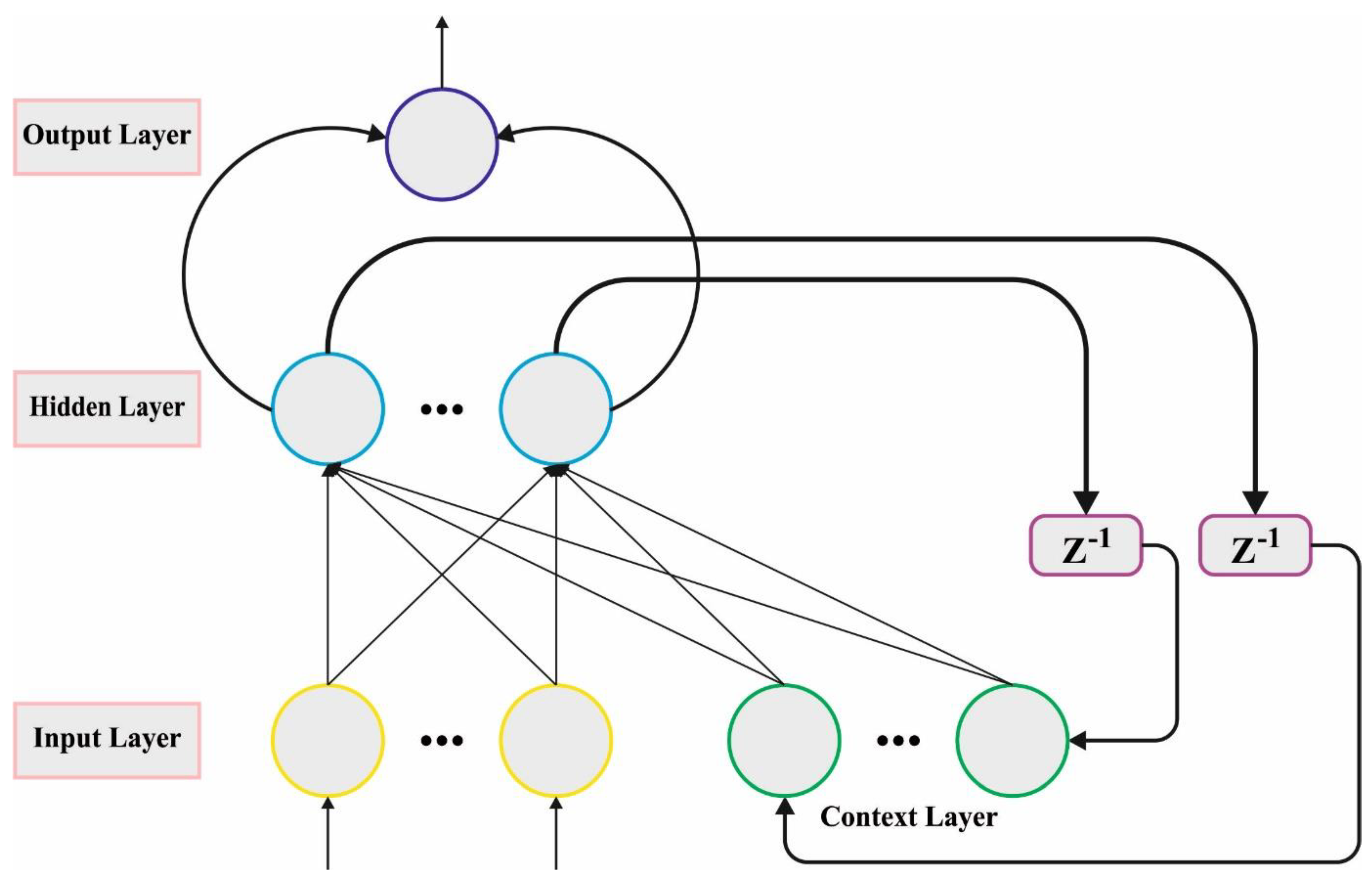
3.2. Road Damage Classification: Optimal ENN Model

Once a road damage was identified, the next stage involved its classification using the ENN model. The ENN technique comprises hidden, input, context, and output layers [24]. The major configuration of the ENN module is analogous to that of the FFNN as regards the connections, whereas the context layers are the same as in the MLP. The context layer obtains the input from the hidden state and stores earlier values of the hidden layer. $W_h^i,$ $W_h^c,$ $W_h^0$ represent output weight, external input, and context weight matrixes. Figure 2 depicts the infrastructure of the ENN. The dimension of the output and input layers are characterized by $n$, that is, the dimension of the context layer represents $m$, and $x^1\left(t\right)={[x_1^1\left(t\right),x_2^1\left(t\right),\dots .,x_n^1\left(t\right)]}^T$, $y\left(t\right)={[y_1\left(t\right), y_2\left(t\right), \dots , y_n\left(t\right)]}^T$.

The input unit of the ENN can be as follows:

$$u_i\left(l\right)=e_i\left(l\right), i=1,2, \dots , n$$

(1)

Now, $l$ defines the input and output units at the $l$ round in the following:

$$\begin{array}{l}{v}_k\left(l\right)={\displaystyle {\displaystyle \sum }_{j=1}^N}{\omega }_{kj}^1\left(l\right)x_j^c\left(l\right)+{\displaystyle {\displaystyle \sum }_{i=1}^n}{\omega }_{ki}^2\left(l\right)u_i\left(l\right)\\ k=1,2, \dots , N \end{array}$$

(2)

Here, $x_j^c\left(l\right)$ defines the signals that are disseminated from the $k$-$th$ context node, ${\omega }_{kj}^1\left(l\right)$ describes the $i$-$th$ and $j$-$th$ weights of the hidden state directed from the $o$-$th$ nodes. Eventually, the outcome of the hidden states is obtained into the context layer, as shown below:

$$W_k\left(l\right)=f_0\left({\overline{v}}_k\left(l\right)\right)$$

(3)

Now,

$${\overline{v}}_k\left(l\right)=\frac{v_k\left(l\right)}{\max \left\{v_k\left(l\right)\right\}}$$

(4)

The above-mentioned formula denotes the normalized value of the hidden state as

$$C_k\left(l\right)=\beta C,\left(l-1\right)+W_k\left(l-1\right), k=1,2, \dots , N$$

(5)

In Equation (5), $W_k$ specifies the gain of self-connected feedback among [0, 1]. Eventually, the output unit in the network is:

$$y_0\left(l\right)={\displaystyle \sum }_{k=1}^N{\omega }_{ok}^3\left(l\right)W_k,\left(l\right), 0=1,2, \dots , n$$

(6)

In the above expression, ${\omega }_{ok}^3$ describes the connection weight from the $k$-$th$ into the $o$-$th$ layer.

In the final stage, the HGS algorithm was enforced to tuning the parameters relevant to the ENN model. Hunger produces internal animal requirements that induce animals to forage [25]. There is no doubt that different stimuli affect the life of animals and that animals lacking calories will seek food. To satisfy its needs, the animals forage continuously in their environments, alternating between competitive, exploratory, and defensive activities. The animals can alter dynamically their search patterns based on their hunger level. Once hunger is high, separate animal may seek food together in a restricted region moving in the same direction and concentrating in areas with high resources. This efficiently stimulates animals to organize socially. This approach becomes well-established once animals with dissimilar hunger levels are dispersed in similar regions. The mathematical mechanism and model regarding the described state of hunger can be defined as follows. The key stages of the HGS are shown below.

1.

Population initialized: to determine the first location for optimal search, the population will be initialized. The HGS approach makes use of the $N$ real-valued vector of dimension $D$, and all the members of the population are denoted by $X_i={[X_{i1}{X}_{i2}\dots X_{iD}]}_r^{T}i=1,2,\dots N.$ In the original HGS model, each population member is considered to conform to a mean and probabihty distribution with the subsequent formula

$$X_{N\times D}=rand\left(N,D\right)\times \left(ub-lb\right)+lb$$

(7)

In Equation (7), $N\times D$ signifies a Euclidean space, $N$ signifies the population count, and $D$ represents the dimension of space; $ub$ and $lb$ represent the upper and the lower bounds of the search region.

2.

Approach food: This phase can be described as follows

$$\overrightarrow{X\left(t+1\right)}=\{\begin{array}{l}\overrightarrow{X\left(t\right)}\cdot \left(1+randn\left(1\right)\right),r l\hfill \\ \overrightarrow{W_1}\cdot \overrightarrow{X_b}+\overrightarrow{R}\cdot \overrightarrow{W_2}|\overrightarrow{X_b}-\overrightarrow{X\left(t\right)}|, r_1\rangle l, r_2\rangle E\hfill \\ \overrightarrow{W_1}\cdot \overrightarrow{X_b}-\overrightarrow{R}\cdot \overrightarrow{W_2}\left|\overrightarrow{X_b}-\overrightarrow{X\left(t\right)}\right|,r l,r E\hfill \end{array}$$

(8)

In Equation (8), $\overrightarrow{X\left(t\right)}$ represents the existing individual. $\overrightarrow{X_b}$ signifies the position of the individuals with better fitness values; randn (l) follows a standard distribution having the mean of $0$ and the variance of 1; $r1$ and $r2$ indicate arbitrary numbers in the range $\left[-1,1\right]. \overrightarrow{R}$ indicates the values in the range [$-a,a].$ $\overrightarrow{W_1}$ and $\overrightarrow{W_2}$ characterize the hunger weight. The variable $l$ is intended for facilitating the application to a varied population, upgrading the existing search agent, and thereby enhancing the algorithm performance. The $E$ parameter can efficiently control the direction in the searching region and thereby increase the diversity of the population; it is determined as follows

$$E=sech\left(\left|F_i-BF\right|\right)$$

(9)

In Equation (9), $i$ represents a positive integer within $[$1, $N]$, and $F_i$ signifies the fitness of the $i$-$th$ population member. $BF$ signifies the best fitness attained so far. Sech is a function (sech $\left(x\right)=2/\left(e^{\chi }+e^{-x}\right))$. The variable $\overrightarrow{R}$ is presented to dynamically control the search phase of the search agents

$$\overrightarrow{R}\times a\times rand-a$$

(10)

$$a\times \left(1-\frac{t}{T}\right)$$

(11)

Now, $rand$ represents a random parameter, whose values range is $\left[-1\right];$ $t$ characterizes the iteration count of the existing model, and $T$ denotes the maximal iteration count.

3.

Hunger role: here, the hunger features of the search agent were simulated mathematically. In Equation (8), $\overrightarrow{W_1}$ and $\overrightarrow{W_2}$ characterize the extent of the population starvation, which vigorously controls the upgrade of the search agents’ position.

$\overrightarrow{W_1}$ is determined with Equation (12):

$$\overrightarrow{W_1}\{\begin{array}{l}hungry\left(i\right)\times \frac{N}{SHungry}\times r_4,r_3<l\hfill \\ r_3>l\hfill \end{array}$$

(12)

The equation for $\overrightarrow{W_2}$ in Equation (7) is shown below:

$$\overrightarrow{W_2\left(\iota \right)}=\left(1-exp\left(-\left|hungry\left(i\right)-SHungry\right|\right)\right)\times r_5\times 2$$

(13)

In Equation (13), $hungry$ specifies the level of hunger of all the individuals in the population. $N$ denotes the number of the individuals in the population. $SHungry$ indicates the sum of the hunger levels of all the population associates; $r3,$ $r4,$ and $r5$ indicate random values within $\left[-1,1\right]$ as follows:

$$hungry\left(i\right)=\{\begin{array}{l}0,AllFitness\left(i\right)==BF\hfill \\ hungry\left(i\right)+H, AllFitness \left(\right)!=BF\hfill \end{array}$$

(14)

For better modelling the hunger levels of every population member, the hunger level of every population member was interconnected to the fitness values, where AllFitness(i) indicates the fitness value of $i$-$th$ population member of existing iteration; $BF$ denotes better fitness values of the population till the existing iteration. When the fitness values of the existing search affiliates are equivalent to $BF$, it indicates that each associate is sated and does not feel hunger. In contrast, if the affiliate is in a starvation state, the starvation activation variable $H$ is determined:

$$TH\frac{F_i-BF}{WF-BF}\times r_6\times 2\times \left(ub-lb\right)$$

(15)

$$H=\{\begin{array}{l}LH\times \left(1+r\right), TH<LH\hfill \\ TH,TH\ge LH\hfill \end{array}$$

(16)

Now, $F_i$ indicates the fitness values of every individual in the population. $BF$ and $WF$ show the best and worst fitness values of the individuals attained till the existing iteration. The upper and the lower bounds of the potential area are denoted as $ub$ and $lb$; $r6$ indicates a random value within the range $\left[1,1\right]$. The sensation of hunger $H$ was fixed to its lowest limit, $LH$, that generally takes the value of 100.

4. Experimental Validation

The proposed model was simulated using the Python 3.6.5 tool. The proposed model was experimented on PC i5-8600k, GeForce 1050Ti 4GB, 16GB RAM, 250GB SSD, and 1TB HDD. The parameter settings were: learning rate, 0.01, dropout, 0.5, batch size, 5, epoch count, 50, and activation, ReLU. In this study, the road damage classification results of the RDD–HGSENN method were assessed using the dataset of 4000 images as reported in

Table 1. Dataset details.

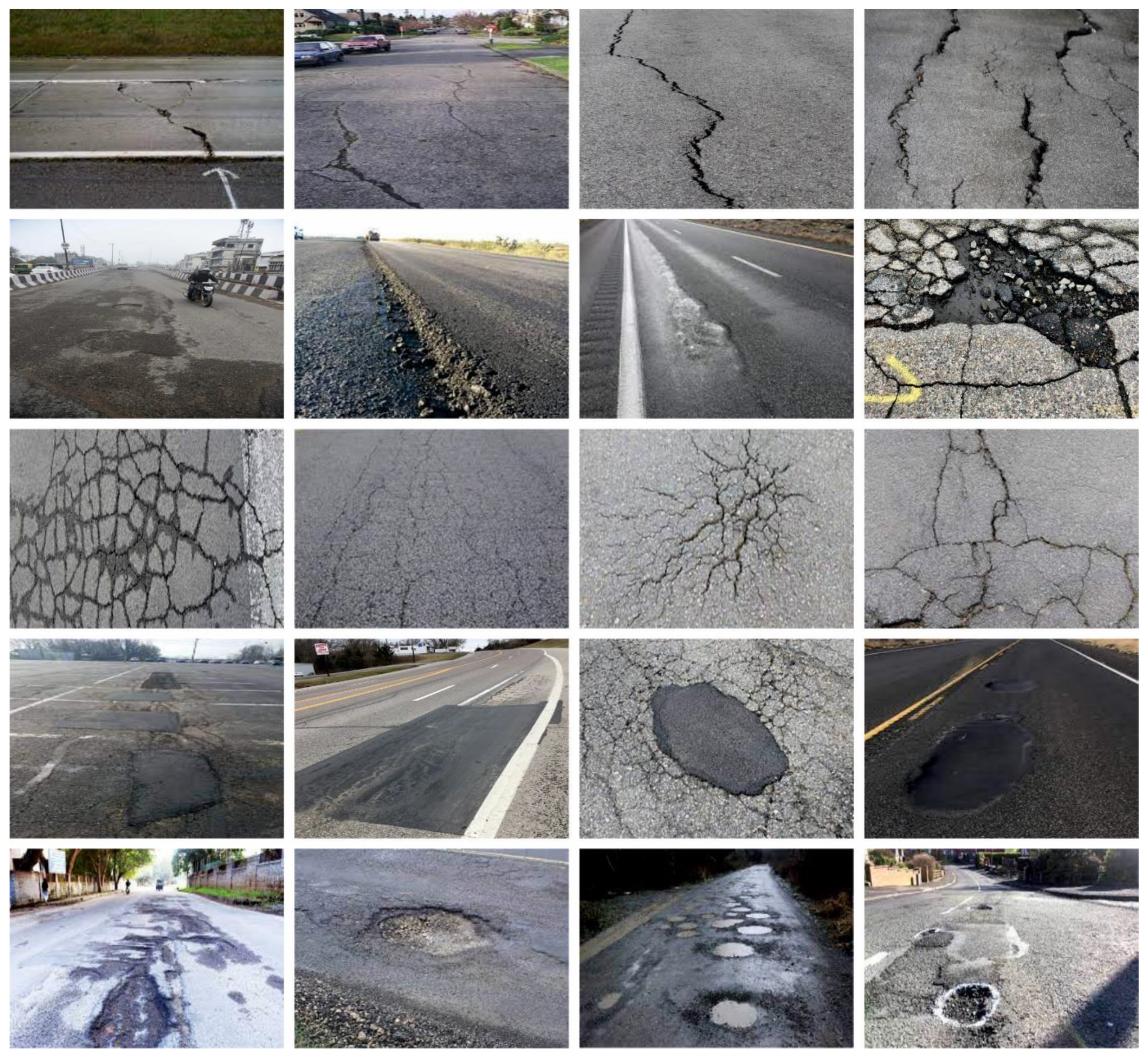
Class	No. of Samples
Linear Cracks	1000
Peeling	1000
Alligator Cracks	1000
Potholes	1000
Total Number of Samples	4000

. Figure 3 shows some sample images.

The road damage classification results of the RDD–HGSENN model were examined using a confusion matrix shown in Figure 4. The confusion matrix portrayed that the RDD–HGSENN model had properly recognized all types of road damages.

Table 2. Road damage detection outcome of the RDD–HGSENN system for 80:20 of the TR/TS databases.

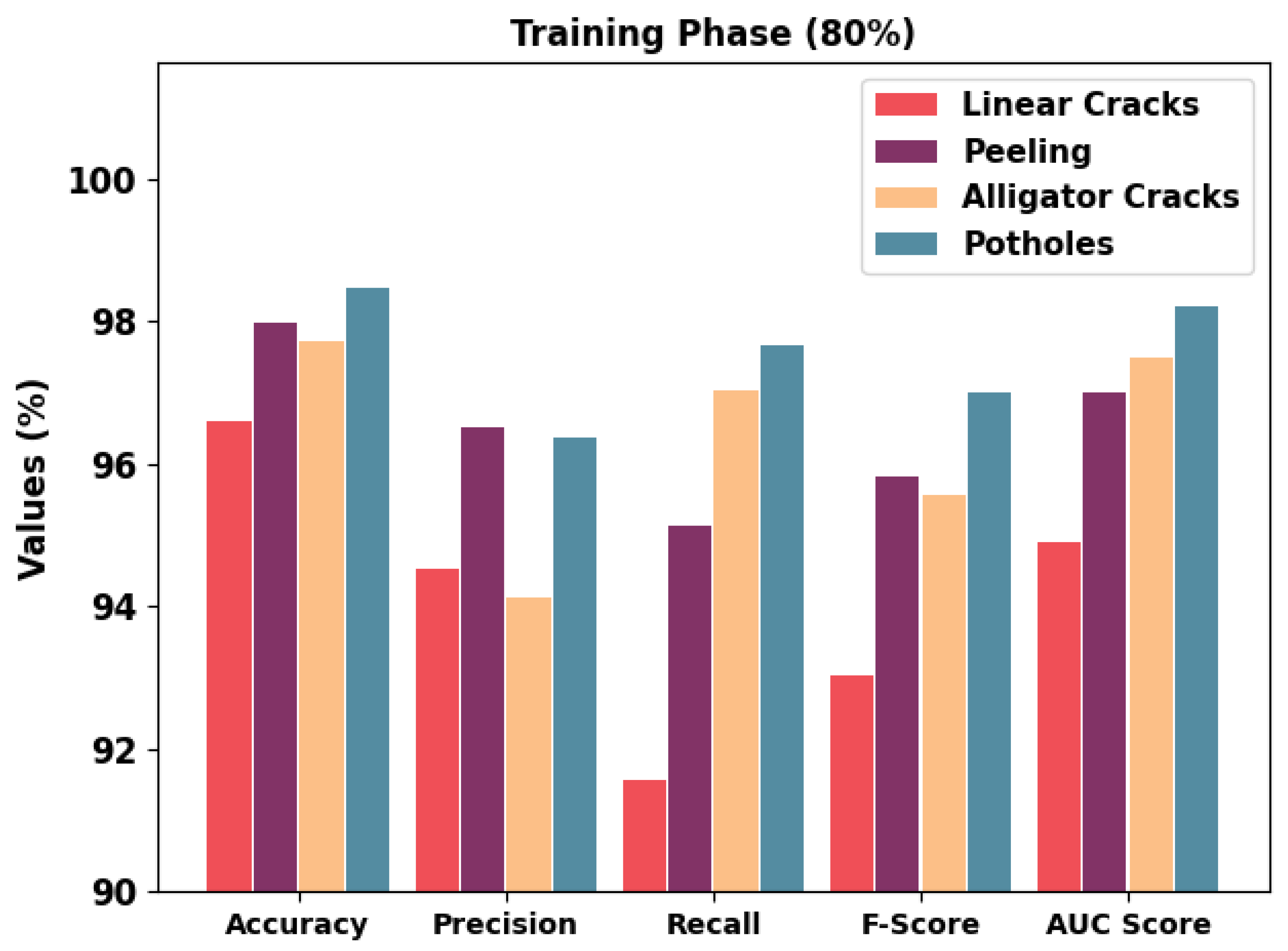
Class	Accuracy	Precision	Recall	F-Score	AUC Score
Training Phase (80%)
Linear Cracks	96.59	94.53	91.55	93.02	94.90
Peeling	97.97	96.50	95.14	95.81	97.01
Alligator Cracks	97.72	94.13	97.04	95.56	97.49
Potholes	98.47	96.37	97.67	97.01	98.21
Average	97.69	95.38	95.35	95.35	96.90
Testing Phase (20%)
Linear Cracks	96.63	93.69	93.24	93.46	95.52
Peeling	98.38	98.12	95.87	96.98	97.59
Alligator Cracks	98.88	96.41	98.95	97.66	98.90
Potholes	98.62	96.77	97.30	97.04	98.16
Average	98.13	96.25	96.34	96.29	97.54

provides the road damage detection output of the RDD–HGSENN method for 80% of the TR database and 20% of the TS database. Figure 5 showcases the road damage classification results of the RDD–HGSENN method for 80% of the TR database. The results showed that the RDD–HGSENN model identified all distinct kinds of road damage. For instance, the RDD–HGSENN model detected linear cracks with an $acc{u}_y$ of 96.59% and peeling with an $acc{u}_y$ of 97.97%. Finally, the RDD–HGSENN approach detected potholes with an $acc{u}_y$ of 98.47%.

Figure 6 displays the road damage classification results of the RDD–HGSENN method with 20% of the TS database. The results displayed that the RDD–HGSENN algorithm identified all distinct kinds of road damages. For example, the RDD–HGSENN technique detected linear cracks with an $acc{u}_y$ of 96.63% and peeling with an $acc{u}_y$ of 98.38%. Finally, the RDD-HGSENN approach identified potholes with an $acc{u}_y$ of 98.62%.

Table 3. Road damage detection outcome of the RDD–HGSENN system for 70:30 of the TR/TS databases.

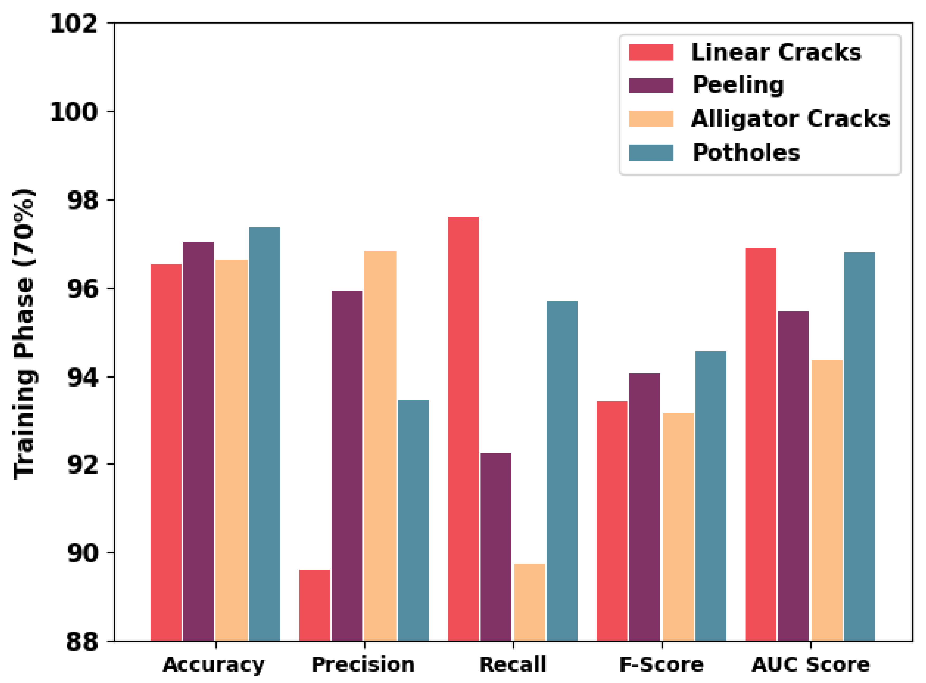
Class	Accuracy	Precision	Recall	F-Score	AUC Score
Training Phase (70%)
Linear Cracks	96.54	89.61	97.60	93.43	96.89
Peeling	97.04	95.91	92.26	94.05	95.46
Alligator Cracks	96.64	96.81	89.73	93.14	94.36
Potholes	97.36	93.45	95.68	94.55	96.78
Average	96.89	93.94	93.82	93.79	95.87
Testing Phase (30%)
Linear Cracks	97.17	91.64	97.27	94.37	97.20
Peeling	97.92	96.48	94.81	95.64	96.86
Alligator Cracks	97.50	98.14	91.35	94.62	95.40
Potholes	98.58	96.43	98.48	97.44	98.55
Average	97.79	95.67	95.48	95.52	97.00

presents the road damage detection output of the RDD–HGSENN system with 70% of the TR database and 30% of the TS database. Figure 7 portrays the road damage classification outcomes of the RDD–HGSENN approach with 70% of the TR database. The results displayed the RDD–HGSENN method identified all distinct kinds of road damage. For example, the RDD–HGSENN technique detected linear cracks with an $acc{u}_y$ of 96.54% and peeling with an $acc{u}_y$ of 97.04%. Finally, the RDD–HGSENN technique detected potholes with an $acc{u}_y$ of 97.36%.

Figure 8 exhibits the road damage classification results of the RDD–HGSENN technique with 30% of the TS database. The results displayed the RDD–HGSENN technique has identified all distinct kinds of road damage. For example, the RDD–HGSENN approach detected linear cracks with an $acc{u}_y$ of 97.17% and peeling with an $acc{u}_y$ of 97.92%. Finally, the RDD–HGSENN approach detected potholes with an $acc{u}_y$ of 98.58%.

The training accuracy (TRA) and validation accuracy (VLA) reached by the RDD–HGSENN approach using the test database are shown in Figure 9. The simulation result indicates that the RDD–HGSENN methodology reached high values of TRA and VLA. In addition, the VLA was higher than the TRA.

The training loss (TRL) and validation loss (VLL) attained by the RDD–HGSENN system using the test database are shown in Figure 10. The simulation results indicated the RDD–HGSENN approach exhibited low values of TRL and VLL. In particular, the VLL was lower than the TRL.

A clear precision–recall examination of the RDD–HGSENN method using the test database is depicted in Figure 11. The figure shows that the RDD–HGSENN system resulted in improved precision–recall values in every class label.

A brief ROC examination of the RDD–HGSENN system using the test database is portrayed in Figure 12. The results indicated that the RDD–HGSENN was able to distinguish different classes in the test database.

At last, an extensive comparative study of the RDD–HGSENN model with recent DL models, reported in

Table 4. Comparative analysis of the RDD–HGSENN system with the currently used DL approaches.

Methods	Accuracy	Precision	Recall	F-Score
RDD-HGSENN	98.13	96.25	96.34	96.29
MobileNet	90.03	90.88	88.97	89.15
AlexNet	92.84	93.52	93.83	92.95
GoogleNet	91.47	92.23	91.33	91.39
RetinaNet	90.70	89.45	89.80	90.17

, was conducted [26]. Figure 13 reports a detailed $acc{u}_y$ assessment of the RDD–HGSENN method and the existing methods. The figure shows that the RDD–HGSENN method gained a higher $acc{u}_y$ of 98.13% compared to the MobileNet, AlexNet, GoogleNet, and RetinaNet models, whose $acc{u}_y$ was 90.03%, 92.84%, 91.47%, and 90.70%, respectively.

Finally, comparative results of the RDD–HGSENN model are provided in terms of $pre{c}_n$, $rec{a}_l$, and $F_{score}$, as shown in Figure 14. The results demonstrated that the MobileNet and RetinaNet models showed lower classification outcomes.

The AlexNet and GoogleNet methods reached a realistic performance. However, the RDD–HGSENN model showed enhanced results, with maximum $pre{c}_n$, $rec{a}_l$, and $F_{score}$ of 96.25%, 96.34%, and 96.29%, respectively. Therefore, the RDD–HGSENN model can be employed for an accurate road damage classification.

5. Conclusions

In this article, a new RDD–HGSENN method was developed for road damage detection using high-resolution RSIs. The presented RDD–HGSENN technique majorly focuses on the detection and classification of road damages using remote sensing images. In the presented RDD–HGSENN technique, the RetinaNet model is applied for damage detection on a road. Moreover, the RDD–HGSENN technique performs road damage classification using the ENN model. Finally, the HGS algorithm was applied to tune the ENN parameters. To examine the enhanced outcomes of the presented RDD–HGSENN technique, a comprehensive set of simulations were conducted. The experimental outcomes demonstrated the improved performance of the RDD–HGSENN technique with respect to recent approaches, with a maximum accuracy of 98.13%. In the future, we plan to extend the RDD–HGSENN technique by the use of advanced DL classifiers. In addition, the computational complexity of the proposed model can be examined in future.

References

- Cao, M.T.; Tran, Q.V.; Nguyen, N.M.; Chang, K.T. Survey on performance of deep learning models for detecting road damages using multiple dashcam image resources. Adv. Eng. Inform. 2020, 46, 101182. [Google Scholar] [CrossRef]
- Hruza, P.; Mikita, T.; Tyagur, N.; Krejza, Z.; Cibulka, M.; Prochazkova, A.; Patocka, Z. Detecting forest road wearing course damage using different methods of remote sensing. Remote. Sens. 2018, 10, 492. [Google Scholar] [CrossRef]
- Li, J.; Zhao, X.; Li, H. April. Method for detecting road pavement damage based on deep learning. In Health Monitoring of Structural and Biological Systems XIII; Fromme, P., Su, Z., Eds.; SPIE: Bellingham, WA, USA, 2019; Volume 10972, pp. 517–526. [Google Scholar]
- Azimi, M.; Eslamlou, A.D.; Pekcan, G. Data-driven structural health monitoring and damage detection through deep learning: State-of-the-art review. Sensors 2020, 20, 2778. [Google Scholar] [CrossRef] [PubMed]
- Arya, D.; Maeda, H.; Ghosh, S.K.; Toshniwal, D.; Mraz, A.; Kashiyama, T.; Sekimoto, Y. Deep learning-based road damage detection and classification for multiple countries. Autom. Constr. 2021, 132, 103935. [Google Scholar] [CrossRef]
- Yin, J.; Qu, J.; Huang, W.; Chen, Q. Road damage detection and classification based on multi-level feature pyramids. KSII Trans. Internet Inf. Syst. (TIIS) 2021, 15, 786–799. [Google Scholar]
- Heidari, M.J.; Najafi, A.; Borges, J.G. Forest Roads Damage Detection Based on Objected Detection Deep Learning Algorithms. 2022. [Google Scholar] [CrossRef]
- Van Der Horst, B.B.; Lindenbergh, R.C.; Puister, S.W.J. Mobile laser scan data for road surface damage detection. Int. Arch. Photogramm. Remote Sens. Spat. Inf. Sci. 2019, 42, 1141–1148. [Google Scholar] [CrossRef]
- Shim, S.; Kim, J.; Lee, S.W.; Cho, G.C. Road surface damage detection based on hierarchical architecture using lightweight auto-encoder network. Autom. Constr. 2021, 130, 103833. [Google Scholar] [CrossRef]
- Angulo, A.; Vega-Fernández, J.A.; Aguilar-Lobo, L.M.; Natraj, S.; Ochoa-Ruiz, G. Road damage detection acquisition system based on deep neural networks for physical asset management. In Proceedings of the 18th Mexican International Conference on Artificial Intelligence, MICAI 2019, Xalapa, Mexico, 27 October–2 November 2019; Springer: New York, NY, USA, 2019; pp. 3–14. [Google Scholar]
- Jia, J.; Sun, H.; Jiang, C.; Karila, K.; Karjalainen, M.; Ahokas, E.; Khoramshahi, E.; Hu, P.; Chen, C.; Xue, T.; et al. Review on active and passive remote sensing techniques for road extraction. Remote Sens. 2021, 13, 4235. [Google Scholar] [CrossRef]
- Chen, Z.; Deng, L.; Luo, Y.; Li, D.; Junior, J.M.; Gonçalves, W.N.; Nurunnabi, A.A.M.; Li, J.; Wang, C.; Li, D. Road extraction in remote sensing data: A survey. Int. J. Appl. Earth Obs. Geoinf. 2022, 112, 102833. [Google Scholar] [CrossRef]
- Shao, Z.; Zhou, Z.; Huang, X.; Zhang, Y. MRENet: Simultaneous extraction of road surface and road centerline in complex urban scenes from very high-resolution images. Remote Sens. 2021, 13, 239. [Google Scholar] [CrossRef]
- Zhang, L.; Lan, M.; Zhang, J.; Tao, D. Stagewise unsupervised domain adaptation with adversarial self-training for road segmentation of remote-sensing images. IEEE Trans. Geosci. Remote Sens. 2021, 60, 1–13. [Google Scholar] [CrossRef]
- Chen, Z.; Wang, C.; Li, J.; Fan, W.; Du, J.; Zhong, B. Adaboost-like End-to-End multiple lightweight U-nets for road extraction from optical remote sensing images. Int. J. Appl. Earth Obs. Geoinf. 2021, 100, 102341. [Google Scholar] [CrossRef]
- Shim, S.; Kim, J.; Lee, S.W.; Cho, G.C. Road damage detection using super-resolution and semi-supervised learning with generative adversarial network. Autom. Constr. 2022, 135, 104139. [Google Scholar] [CrossRef]
- Zhao, K.; Liu, J.; Wang, Q.; Wu, X.; Tu, J. Road Damage Detection From Post-Disaster High-Resolution Remote Sensing Images Based on TLD Framework. IEEE Access 2022, 10, 43552–43561. [Google Scholar] [CrossRef]
- Yuan, Y.; Yuan, Y.; Baker, T.; Kolbe, L.M.; Hogrefe, D. FedRD: Privacy-preserving adaptive Federated learning framework for intelligent hazardous Road Damage detection and warning. Future Gener. Comput. Syst. 2021, 125, 385–398. [Google Scholar] [CrossRef]
- Fan, R.; Liu, M. Road damage detection based on unsupervised disparity map segmentation. IEEE Trans. Intell. Transp. Syst. 2019, 21, 4906–4911. [Google Scholar] [CrossRef]
- Fan, R.; Cheng, J.; Yu, Y.; Deng, J.; Giakos, G.; Pitas, I. Long-awaited next-generation road damage detection and localization system is finally here. In Proceedings of the 2021 29th European Signal Processing Conference (EUSIPCO), Dublin, Ireland, 23–27 August 2021; IEEE: Piscataway, NJ, USA, 2021; pp. 641–645. [Google Scholar]
- Kortmann, F.; Talits, K.; Fassmeyer, P.; Warnecke, A.; Meier, N.; Heger, J.; Drews, P.; Funk, B. Detecting various road damage types in global countries utilizing faster r-cnn. In Proceedings of the 2020 IEEE International Conference on Big Data (Big Data), Atlanta, GA, USA, 10–13 December 2020; IEEE: Piscataway, NJ, USA, 2020; pp. 5563–5571. [Google Scholar]
- Izadi, M.; Mohammadzadeh, A.; Haghighattalab, A. A new neuro-fuzzy approach for post-earthquake road damage assessment using GA and SVM classification from QuickBird satellite images. J. Indian Soc. Remote Sens. 2017, 45, 965–977. [Google Scholar] [CrossRef]
- Hill, C. Automatic Detection of Vehicles in Satellite Images for Economic Monitoring. Doctoral Dissertation, University of South Florida, Tampa, FL, USA, 2021. [Google Scholar]
- Sitharthan, R.; Krishnamoorthy, S.; Sanjeevikumar, P.; Holm-Nielsen, J.B.; Singh, R.R.; Rajesh, M. Torque ripple minimization of PMSM using an adaptive Elman neural network-controlled feedback linearization-based direct torque control strategy. Int. Trans. Electr. Energy Syst. 2021, 31, 12685. [Google Scholar]
- Zhou, X.; Gui, W.; Heidari, A.A.; Cai, Z.; Elmannai, H.; Hamdi, M.; Liang, G.; Chen, H. Advanced Orthogonal Learning and Gaussian Barebone Hunger Games for Engineering Design. J. Comput. Des. Eng. 2022, 9, 1699–1736. [Google Scholar] [CrossRef]
- Ochoa-Ruiz, G.; Angulo-Murillo, A.A.; Ochoa-Zezzatti, A.; Aguilar-Lobo, L.M.; Vega-Fernández, J.A.; Natraj, S. An asphalt damage dataset and detection system based on retinanet for road conditions assessment. Appl. Sci. 2020, 10, 3974. [Google Scholar] [CrossRef]