Transferability of Recursive Feature Elimination (RFE)-Derived Feature Sets for Support Vector Machine Land Cover Classification

Abstract

Remote sensing analyses frequently use feature selection methods to remove non-beneficial feature variables from the input data, which often improve classification accuracy and reduce the computational complexity of the classification. Many remote sensing analyses report the results of the feature selection process to provide insights on important feature variable for future analyses. Are these feature selection results generalizable to other classification models, or are they specific to the input dataset and classification model they were derived from? To investigate this, a series of radial basis function (RBF) support vector machines (SVM) supervised machine learning land cover classifications of Sentinel-2A Multispectral Instrument (MSI) imagery were conducted to assess the transferability of recursive feature elimination (RFE)-derived feature sets between different classification models using different training sets acquired from the same remotely sensed image, and to classification models of other similar remotely sensed imagery. Feature selection results for various training sets acquired from the same image and different images widely varied on small training sets (n = 108). Variability in feature selection results between training sets acquired from different images was reduced as training set size increased; however, each RFE-derived feature set was unique, even when training sample size was increased over 10-fold (n = 1895). The transferability of an RFE-derived feature set from a high performing classification model was, on average, slightly more accurate in comparison to other classification models of the same image, but provided, on average, slightly lower accuracies when generalized to classification models of other, similar remotely sensed imagery. However, the effects of feature set transferability on classification accuracy were inconsistent and varied per classification model. Specific feature selection results in other classification models or remote sensing analyses, while useful for providing general insights on feature variables, may not always generalize to provide comparable accuracies for other classification models of the same dataset, or other, similar remotely sensed datasets. Thus, feature selection should be individually conducted for each training set within an analysis to determine the optimal feature set for the classification model.

1. Introduction

Feature selection techniques are frequently used in remote sensing analyses to increase the prediction accuracy and interpretability of machine learning classification algorithms through the removal of redundant, noisy, irrelevant, or non-beneficial predictor variables from the training dataset or feature space, often through identifying and selecting an optimal combination of features that maximizes the accuracy of a given classification model of interest as measured using an accuracy metric (e.g., overall accuracy, kappa statistic, area under the receiver operating characteristic curve (AUC ROC), or F1 score) [1,2,3].

Feature selection has been found to be particularly beneficial for high dimensional datasets, such as multispectral imagery [4,5] or hyperspectral imagery [6,7,8], which often contain hundreds of spectral and textural features, as well as geographic object-based image analysis (GEOBIA) [9,10], which uses image segmentation to group together similar adjacent pixels into discrete non-overlapping image objects, which then serve as the unit of analysis [11]. In addition to spectral and textural information, image segmentation in GEOBIA also generates geometric information, which further increases the dimensionality of the feature space.

In many applied analyses, the results of the feature selection process, which are usually provided in the form of feature importance rankings [12,13,14,15], or a listing of the features contained in the optimized feature set [9,10], are typically included as part of the analysis results, often with the intention of providing insights on selecting image features for use in future analyses. While feature selection results can be useful for gaining insights on which image features were useful or beneficial for the classification, it is unclear if such results can be extended to other classification models trained from different training sets, or even other, similar remotely sensed data. This brings into question if a feature set is able to be generalized beyond the dataset it was derived from. Essentially, are specific feature sets derived from feature selection processes transferrable between different classification models? Additionally, are feature selection results consistent between training sample sets acquired from the same image, or are feature selection results largely specific to the training data?

Most prior research on feature selection generally focuses on the comparisons of feature selection methods [1,16,17], or the effects of feature selection processes on various machine learning [6,18] or deep learning classifications [13] of remotely sensed data. However, there has been comparably minimal research on the transferability of feature selection results between similar classification models of the same remotely sensed dataset, or between similar remotely sensed datasets.

To provide insights on this issue, this paper focuses on investigating the transferability (which in this context refers to the application of an optimized feature set from one classification model to another classification model trained from a different training set) of optimized feature sets derived from feature selection processes to other classification models of the same remotely sensed dataset, and to other similar remotely sensed datasets, through a series of supervised machine learning land cover classifications of medium spatial resolution Sentinel-2A multispectral imagery within a GEOBIA framework.

Furthermore, this analysis employs recursive feature elimination (RFE), a greedy, backwards selection approach, widely used for feature selection in remote sensing analyses [17,19,20]. RFE was applied to generate optimal feature sets for a series of land cover classifications generated by a radial basis function (RBF) support vector machine (SVM) classifier of three temporally and environmentally similar 10 m spatial resolution Sentinel-2A Multispectral Instrument (MSI) images collected over unique geographic extents within a geographic object-based image analysis.

2. Materials and Methods

2.1. Study Areas and Remotely Sensed Data

Three study areas in the eastern United States were selected for this analysis (Figure 1). The first study site, referred to as the “Delaware” study area, is centered around the Delaware Bay and surrounding coastal areas, including a portion of southern New Jersey, eastern Maryland, and most of Delaware state. This area includes the cities of Dover, Delaware, and Millville and Vineland, New Jersey. The second study site, referred to as the “Virginia” study area, is along the Chesapeake Bay coastal area within the state of Virginia, including the Rappahannock, York, and James rivers, as well as the Newport News, Virginia, metropolitan area. The third study site, referred to as the “North Carolina” study area, is contained within the coastal plains region of the state of North Carolina, including the western portion of the Croatoan National Forest, as well as the New River, and coastal towns such as Jacksonville and Topsail Beach, in addition to northern parts of the metropolitan area of Wilmington, North Carolina (Figure 1).

The study sites were chosen in part due to their environmental and ecological similarity, as all three study sites are primarily within the same Level II ecoregion—Middle Atlantic Coastal Plain, as defined by the United States Environmental Protection Agency (EPA) [21]. In addition, all three study sites contain both forested and urban areas, as well as significant quantities of water, coastal, and wetland areas. An additional factor for the selection of the three study sites was the availability of cloud-free Sentinel-2A imagery that was all acquired within a relatively narrow timeframe. While each study area is geographically distinct, the environmental similarity between the study sites and availability of imagery were ideal for assessing the transferability of feature selection results to similar remotely sensed datasets. Six land cover classifications were mapped for this analysis: forest, grassland, exposed soil, developed, wetlands, and water (

Table 1. Description of land cover classes.

Name	Description
Forest	Areas dominated by trees, woody vegetation
Grassland	Non-woody vegetation and herbaceous areas
Exposed Soil	Bare soil, tilled agricultural fields, beach sands
Developed	Urban and sub-urban areas, roads, other synthetic impervious surfaces
Wetlands	Swamps, marshes, inundated soils
Water	Natural and synthetic waterbodies

).

2.2. Remotely Sensed Data and Preprocessing

Sentinel-2A MSI satellite imagery was used as the remotely sensed data for this analysis. As GEOBIA methods have proven to be particularly beneficial for higher spatial resolution imagery [1,22], only the 10 m bands, Band 2—blue (0.49 μm), Band 3—green (0.56 μm), Band 4—red (0.665 μm), and Band 8—near infrared (NIR) (0.842 μm) were used. All three images were 10,980 rows by 10,980 columns, with a pixel size of 10 m, and a 12-bit radiometric resolution. All images were cloud-free, and acquired in September 2021, during leaf-on conditions. Due to the temporal similarity of all three images, phenological variations between images were minimal. Level-1C Sentinel-2 imagery was available for the three study areas, which represents top of atmosphere (TOA) reflectance values. Atmospheric correction was applied to the three Level-1C orthoimages using the Sen2Cor software, version 2.1, to obtain Level-2A data containing bottom of atmosphere (BOA) surface reflectance values. Level-2A data is considered to be ideal for basic and applied research activities as further atmospheric correction to the image is not needed [23].

2.3. Experimental Design

To explore the issue of feature set transferability, a series of supervised classifications and feature selection processes were conducted on each of the three remotely sensed datasets. Image segmentation was applied to the Delaware, Virginia, and North Carolina image datasets to partition each image into a set of discrete image objects. Spectral, textural, and geometric features were then calculated for each image object. Simple random sampling was used to create an initial sample set of image objects (n = 3000) from each image dataset. Samples were manually assigned class membership and verified by the analyst. The holdout method was then used to randomly partition each sample set into training (n = 2103) and test datasets (n = 897) for each image. To prevent data leakage, the test data was used for accuracy assessment only, and not used for feature selection, classification model training, and classifier parameter tuning.

To provide for more robust insights, replication was employed in this analysis through random sub-sampling of the training data of each image dataset to create a series of “small” (n ≈ 107) and “large” (relative to the small training set) (n ≈ 1895) training sets. While the training sets uniquely vary in composition, class proportions were maintained between the sub-sampled training sets within each training sample set size, and image dataset. The purpose of the “small” and “large” training sets was to investigate potential variations in feature selection results on datasets containing high and low amount of overlap in training objects, respectively.

Recursive feature elimination (RFE) was then used to identify the optimal feature set for each large and small training sample set across all image datasets. A series of support vector machine (SVM) classifications were then conducted, including a baseline set of classifications which included the full set of image features, and a set of classifications which used the RFE-optimized feature sets, which represent a standard implementation of feature selection in a classification workflow. Classification accuracy was assessed using the previously mentioned test dataset for each image.

To assess the transferability of RFE-optimized feature sets, the feature set which produced the highest overall accuracy for each image dataset, labeled as the “optimal” feature set, was applied to generate a series of SVM classifications trained from the small and large sample sets for all three images. A single “optimal” feature set was acquired from each set of classifications trained from the large and small sample sets for each image. This method simulates a static feature set which was reported in an applied remote sensing analysis being re-applied to classifications of similar remotely sensed imagery, and classifications of the same image, trained from different training sets. The experimental workflow is described in Figure 2, while following sections describe each process in detail.

2.4. Image Segmentation

The multi resolution segmentation (MRS) algorithm in Trimble eCognition Developer 9.3 was chosen as the image segmentation method [24]. MRS is a region-growing bottom-up segmentation algorithm which partitions raster grids into distinct, non-overlapping image objects using a series of user-specified inputs, including image layer weights, scale, shape, and compactness parameters. Equal weighting was given to all four spectral band layers for the segmentation. The scale parameter was determined through the usage of the estimation of scale parameter (ESP2) tool, which is an automated method for determining optimal scale parameters for the algorithm and dataset [25]. Determining an optimal scale parameter using the ESP2 method is frequently cited as more reproducible than ad hoc trial-and-error methods for determining the scale parameter. Through a series of preliminary segmentations, a scale parameter of 200 was determined to be optimal for all three images. The shape and compactness parameters were left at their defaults of 0.1 and 0.5, respectively, as the adjustment of these parameters did not seem to improve the segmentation in a series of pilot segmentations. The MRS segmentation produced 82,381 image objects for the Delaware dataset, 65,982 image objects for the Virginia dataset, and 70,648 image objects for the North Carolina dataset.

2.5. Image Features

In total, 159 spectral, textural, and geometric features were generated for all image objects. With the exception of a spectral index, namely the normalized difference vegetation index (NDVI), all other features were natively generated within the eCognition Developer environment.

Table 2. List of spectral, textural, and geometric features of the image objects.

Feature Categories	Features
Spectral Features	Mean Blue, Mean Red, Mean Green, Mean NIR, Mode Blue, Mode Red, Mode Green, Mode NIR, Standard Deviation Blue, Standard Deviation Green, Standard Deviation Red, Standard Deviation NIR, Skewness Blue, Skewness Green, Skewness Red, Skewness NIR, Brightness, Max Diff.
Vegetation Indices	NDVI
Textural Features	GLCM Homogeneity (All, 0°, 45°, 90°, 135°), GLCM Contrast (All, 0°, 45°, 90°, 135°), GLCM Dissimilarity (All, 0°, 45°, 90°, 135°), GLCM Entropy (All, 0°, 45°, 90°, 135°), GLCM Entropy (All, 0°, 45°, 90°, 135°), GLCM Ang. 2nd Moment (All, 0°, 45°, 90°, 135°), GLCM Mean (All, 0°, 45°, 90°, 135°), GLCM StdDev (All, 0°, 45°, 90°, 135°), GLCM Correlation (All, 0°, 45°, 90°, 135°), GLDV Ang. 2nd Moment (All, 0°, 45°, 90°, 135°), GLDV Entropy (All, 0°, 45°, 90°, 135°), GLDV Mean (All, 0°, 45°, 90°, 135°), GLDV Contrast (All, 0°, 45°, 90°, 135°)
Geometric Features	Border Length, Shape Index, Border Index, Length, Area, Volume, Roundness, Rectangular Fit, Elliptic Fit, Density, Compactness, Asymmetry

contains the list of features and their associated categories.

2.5.1. Spectral Features

Spectral features are calculated from the individual spectral band layers in the image. The mean, standard deviation, and skewness features represent the first, second, and third statistical moments of the pixel values contained within an image object, and the image object’s relation to other image object’s pixel values. The mode was also calculated as the most common pixel value within each image object for each spectral band. Brightness was calculated as the sum of all mean band values within each object divided by the total number of spectral layers. Another spectral feature, maximum spectral difference, labeled as max diff., is calculated as the maximum difference between mean layer values contained within each image object.

$$\mathrm{Max} \mathrm{diff}=\frac{\underset{i,j\epsilon K^B}{\max }\left| {\overline{C}}_{i }\left(v\right)- {\overline{C}}_j\left(v\right) \right|}{\overline{C} \left(v\right)}$$

(1)

where i and j are the image layers, $\overline{C}\left(v\right)$ is the mean brightness of the image layers, while ${\overline{C}}_{i }\left(v\right)$ and ${\overline{C}}_j\left(v\right)$ are the mean intensity values of image layer i and j, respectively, and $K^B$ are the image layers of positive brightness and weight [26].

2.5.2. Vegetation Indices

The normalized difference vegetation index (NDVI) has been widely demonstrated to be particularly advantageous for land cover classification of multispectral remotely sensed data [27]. NDVI was calculated using the mean Near-Infrared (NIR) and Red band values for each image object. It should be mentioned that while NDVI was used as the sole vegetation index for this analysis, other indices such as the enhanced vegetation index (EVI) [28,29] and soil-adjusted vegetation index (SAVI) [30,31] have been demonstrated as highly beneficial towards land cover classification projects.

2.5.3. Textural Features

Measures of image texture have been widely used in pixel-based and object-based land cover classification of remotely sensed data [22,32,33,34]. The gray-level co-occurrence matrix (GLCM) [35] is frequently used in remote sensing analyses as a statistical technique to extract local textural information from remotely sensed images. The GLCM method converts images to grayscale and extracts spatial features based upon the relationship of brightness values of individual pixels and their immediate neighbors via a kernel, represented as a matrix [36]. Multiple measures can be derived from the GLCM, such has homogeneity, contrast, dissimilarity, entropy, angular second momentum, mean, standard deviation, and correlation (Table 2).

The GLCM can also be computed in all directions or in single directions, such as horizontal (0°), vertical (90°), diagonally from bottom left to top right (45°), and diagonally from top left to bottom right (135°). In this analysis, GLCM measures were computed in all directions, as well as the four individual directions. In addition to GLCM features, four types of gray-level difference vector (GLDV) features, which are derived from GLCM features, were computed as well. GLDV features include GLDV angular second momentum, GLDV entropy, GLDV contrast, and GLDV mean.

2.5.4. Geometric Features

In addition to spectral and textural features derived from the spectral image layers, geometric information relating to the shape and size of image objects were generated. Twelve unique geometric features were used in this analysis, ranging from image object extent measures such as object length, width, and object area—which is simply the number of pixels contained within the image object—among others, to more complex shape-based measures such as object density, compactness, asymmetry, and elliptic fit. Inclusion of geometric features is common in GEOBIA analyses; however, their usefulness towards land cover classification continues to be an active area of research [37,38].

2.6. Sample Selection and Dataset Splitting

Simple random sampling was used to collect 3000 image object samples from each dataset, a total of 9000 samples across all three images. Each sample was manually labeled and verified by the analyst. For classification training and testing purposes, each image object sample set was split into training and test sets using a standard holdout 70/30 split method, with approximately 70% of the data reserved for training, and 30% of the data used for model evaluation and accuracy assessment using the caret R package [39]. As the method implemented in caret attempts to maintain class proportions native to each sample population, there was a small difference in training and test set sizes between the sample sets of the three images (

Table 3. Initial training and test set split sizes.

Dataset	Training	Test
Delaware	2102	898
Virginia	2103	897
North Carolina	2103	897

).

To investigate the variability and transferability of feature selection results between classification models trained from different training sets, new training datasets were constructed through random sub-sampling from the original training set populations for each of the three datasets. Two series of training sets, a “small” training dataset containing 5% of the training set population, and a “large” training dataset containing 90% of the training set population, were developed for all three image datasets. The purpose of the small training sets was to explore the transferability of feature selection results between classifications trained on the same image but using different training samples with minimal overlap in samples between each sample set. The large training sets were designed to explore the transferability of feature selection results between classification models trained from highly similar training sets. For replication purposes, this process was repeated 10 times for each set of large and small training sets (e.g., 10 “Small Delaware”, “Small Virginia”, and “Small North Carolina” training sets, as well as 10 “Large Delaware”, “Large Virginia”, and “Large North Carolina” training sets), resulting in total of 60 unique training sample sets. To randomize the training samples in each sample set, different pseudo-random seed values were used during the sub-sampling process for each training set, which ensured a unique sub-sampling split. To ensure that class sizes were consistent between training sets sub-sampled from the same source dataset, class proportions were maintained between each series of large and small training sets of the three remotely sensed datasets. The composition of each training set series is contained in

Table 4. Large and small training sets via random sub-sampling. Note that 10 unique training sample sets were created for each series of training sets.

Source Dataset	Sample Size	# of Training Objects per Class
		Developed	Exposed Soil	Forest	Grassland	Water	Wetlands	Total
Delaware	Small (n = 107)	26	14	16	39	7	5	107
	Large (n = 1894)	463	243	288	694	116	90	1894
Virginia	Small (n = 107)	15	16	32	29	11	4	107
	Large (n = 1895)	265	281	572	521	190	66	1895
North Carolina	Small (n = 108)	17	25	26	30	6	4	108
	Large (n = 1895)	296	448	460	570	102	19	1895

.

2.7. Feature Selection—Recursive Feature Elimination

Recursive feature elimination (RFE) was used as the feature selection method for this analysis. RFE is a wrapper-type feature selection algorithm which identifies optimal combinations of features through generating a series of classification models and iteratively removing features that do not improve classification accuracy. RFE employs backwards selection, meaning that the RFE search process starts with the full feature set, and proceeds to iteratively remove features that do not contribute to or are detrimental to the accuracy of the classification, until the optimal combination of features is found. The implementation of RFE in this analysis was conducted using a 500-tree random forest algorithm (RF-RFE), specifically, the rfFuncs method within the caret R package [39].

Tenfold cross-validation was also employed within the iterative model development of the RFE process. The RFE process was used to determine the optimal feature set for all 60 sample sets. In addition, the optimal feature sets across the iterations of small and large sample sets for each of the three remotely sensed datasets were also identified. The optimal feature set for each sample set (i.e., Delaware Small sample set, Virginia Large sample set) was determined by the classification with the highest overall accuracy. Although the RFE process itself produced the optimal feature set for each sample set, it should be noted that the accuracy values used for identifying the model with the highest accuracy within each training sample set were determined by the final accuracy assessment using the full test dataset, not the internal accuracy metrics reported by the RFE process and the 10-fold cross-validation tuning. Ultimately, 60 individual RFE-derived feature sets were developed (10 Small Delaware, 10 Large Delaware, 10 Small Virginia, 10 Large Virginia, 10 Small North Carolina, 10 Large North Carolina). The single top performing feature set in each group was identified as the “optimal” feature set. For example, of the 10 feature sets within the Large Delaware classifications, the feature set of the classification with the highest accuracy was chosen as the “Del-Optimal” feature set for the large sample set classifications. Thus, six “optimal” feature sets (one for the large training sets and one for the small sample sets for each of the Delaware, Virginia, and North Carolina image datasets) were identified. Figure 3 describes the workflow and implementation of the RFE process in this analysis.

2.8. Cross-Validation Parameter Tuning

Most machine learning algorithms contain a series of user-specified parameters which can drastically affect the results and accuracy of the model. These parameters can be adjusted and optimized for a particular objective. Tuning methods such as cross-validation are often used for parameter tuning through iteratively constructing a series of preliminary classification models to identify classifier parameters which are optimal for the dataset. In this analysis, k-fold (10-fold) cross-validation was used to tune both the random forest classifier used for feature selection within the RFE process, and the support vector machine (SVM) classifier which produced the final classification models. Prior research [40] has demonstrated that k-fold cross-validation is a suitable cross-validation method for parameter tuning of supervised machine learning land cover classifications of remotely sensed data and can provide relatively rapid tuning for classifiers trained from large or small sample sets.

2.9. Support Vector Machine (SVM) Classifications

A support vector machine (SVM) classifier was used for the final classification models in this analysis. SVM uses select portions of the training data, called support vectors, to identify a linear hyperplane boundary which is used to separate classes within the feature space [41]. In instances where the classes are not linearly separable, SVM can employ the kernel trick, which can transform the feature space to higher dimension where a linear hyperplane boundary between classes can be found [42,43]. The specific implementation of SVM used in this analysis is the radial basis function kernel (RBF). RBF-SVM is commonly used in a variety of remote sensing analyses including land cover classification, as well as basic and applied studies employing feature selection [1,17]. As the purpose of this analysis was to investigate feature set variability and transferability between classification models, rather than a comparative analysis between multiple types of machine learning classifiers, for simplicity, only a single machine learning algorithm, SVM was chosen for this analysis. Other classifiers such as random forests [44] and neural networks [45] are also common in remote sensing analyses [46,47,48,49,50] and could be applicable for this analysis.

The SVM classifications in this analysis can be divided into several groups:

• The first group of classifications were conducted using the original full feature set. This group of classifications serves as a baseline to assess classification performance without any feature set optimization. These set of classifications were labeled as “All”, referring to all features being used for classifier training and tuning.
• The second group of classifications were conducted using an optimized feature set identified by the RFE process that was applied individually to each training sample set. This set of classifications represent the typical implementation of RFE within a classification workflow, where the optimal feature set identified by the RFE for the training set is then applied to the classification. These classifications were labeled as “RFE”.
• The third group of classifications used a feature set derived from the highest performing (in terms of overall map accuracy) classification of the Delaware dataset. It should be mentioned that the optimal feature set was separately identified for classifications trained from large and small sample sets. In essence, two optimal feature sets for the Delaware dataset were identified, the optimal training set identified from the Delaware-RFE classifications trained from the large sample sets, and the Delaware-RFE classifications trained from the small sample sets. Feature set transferability to other classification models was only conducted between classification models trained from sample sets of similar size. This group of classifications is designed to assess the transferability of an optimal feature set to other classifications of the Delaware dataset, but also to classification models of the Virginia and North Carolina Datasets. This group of classifications was labeled as “Del-Optimal”.
• The fourth group of classifications was similar to the third group, except the classifications used the feature sets from the highest performing classifications of the Virginia dataset. This group of classifications is designed to assess the transferability of an optimal feature set to other classifications of the Virginia dataset, but also to classification models of the Delaware and North Carolina Datasets. This group of classifications was labeled as “Vir-Optimal”.
• The fifth group of classifications, like the third and fourth groups, was trained from the most optimal feature sets found among the classifications of the North Carolina dataset. This group of classifications is designed to assess the transferability of an optimal feature set to other classifications of the North Carolina dataset, but also to classification models of the Delaware and Virginia Datasets. This group of classifications was labeled as “NC-Optimal”.

It should be mentioned that each group of classifications contains 10 individual classifications trained from a unique training dataset acquired from random sub-sampling of the original training dataset. In total, 300 classifications (100 classifications for each of the 3 image datasets—Delaware, Virginia, and North Carolina) were conducted for this analysis. An example set of classifications of the Delaware dataset containing all classification groups can be found in

Table 5. Classification groups of the Delaware dataset. Note that the same set of classifications and classification groups were also conducted for the Virginia and North Carolina datasets.

Image Dataset	Classification Group	# of Classifications	Feature Set Used	Training Set Size
Delaware dataset	SVM-Delaware-Large-All	10	Full Feature Set	Large (n = 1894)
	SVM-Delaware-Small-All	10	Full Feature Set	Small (n = 107)
	SVM-Delaware-Large-RFE	10	Individually optimized feature set for each classification	Large (n = 1894)
	SVM-Delaware-Small-RFE	10	Individually optimized feature set for each classification	Small (n = 107)
	SVM-Delaware-Large-Del-Optimal	10	Highest performing Delaware-Large-RFE Classification	Large (n = 1894)
	SVM-Delaware-Small-Del-Optimal	10	Highest performing Delaware-Small-RFE Classification	Small (n = 107)
	SVM-Delaware-Large-Vir-Optimal	10	Highest performing Virginia-Large-RFE Classification	Large (n = 1894)
	SVM-Delaware-Small-Vir-Optimal	10	Highest performing Virginia-Small-RFE Classification	Small (n = 107)
	SVM-Delaware-Large-NC-Optimal	10	Highest performing North Carolina-Large-RFE Classification	Large (n = 1894)
	SVM-Delaware-Small-NC-Optimal	10	Highest performing North Carolina-Small-RFE Classification	Small (n = 107)

.

2.10. Accuracy Assessment

Error was assessed for all classification models using the test set held-out for each image dataset, described in Section 2.6 and Table 2. Classification error was assessed using a series of accuracy metrics commonly used in remote sensing analyses, including overall accuracy, user’s and producer’s accuracies, and the kappa coefficient. Additionally, a series of paired t-tests [51] were conducted to evaluate the statistical significance of differences between matched pairs of overall classification accuracies between classification groups. A p-value smaller than 0.05 indicates a two-sided 95% confidence that the differences in mean classification accuracies between classification groups using different feature sets are statistically significant. Results of the paired t-tests are contained in

Table A1. Paired t-test p-values for Delaware classifications trained from the small training sets. (* Indicates at a 95% confidence that the differences in mean classification accuracies between classification groups are statistically significant, p < 0.05).

Delaware Classifications (Small Training Sets)
	SVM-All	SVM-RFE	SVM-Del-Optimal	SVM-Virginia-Optimal	SVM-NC-Optimal
SVM-All		p < 0.05 *	p < 0.05 *	p < 0.05 *	p < 0.05 *
SVM-RFE			p < 0.05 *	p < 0.05 *	0.6048
SVM-Del-Optimal				p < 0.05 *	p < 0.05 *
SVM-Virginia-Optimal					p < 0.05 *
SVM-NC-Optimal

,

Table A2. Paired t-test p-values for Virginia classifications trained from the small training sets. (* Indicates at a 95% confidence that the differences in mean classification accuracies between classification groups are statistically significant, p < 0.05).

Virginia Classifications (Small Training Sets)
	SVM-All	SVM-RFE	SVM-Del-Optimal	SVM-Virginia-Optimal	SVM-NC-Optimal
SVM-All		p < 0.05 *	p < 0.05 *	p < 0.05 *	p < 0.05 *
SVM-RFE			0.2906	0.2649	p < 0.05 *
SVM-Del-Optimal				0.065	p < 0.05 *
SVM-Virginia-Optimal					p < 0.05 *
SVM-NC-Optimal

,

Table A3. Paired t-test p-values for North Carolina classifications trained from the small training sets. (* Indicates at a 95% confidence that the differences in mean classification accuracies between classification groups are statistically significant, p < 0.05).

North Carolina Classifications (Small Training Sets)
	SVM-All	SVM-RFE	SVM-Del-Optimal	SVM-Virginia-Optimal	SVM-NC-Optimal
SVM-All		p < 0.05 *	p < 0.05 *	p < 0.05 *	p < 0.05 *
SVM-RFE			0.4537	0.7914	p < 0.05 *
SVM-Del-Optimal				0.6669	0.1361
SVM-Virginia-Optimal					p < 0.05 *
SVM-NC-Optimal

,

Table A4. Paired t-test p-values for Delaware classifications trained from the large training sets. (* Indicates at a 95% confidence that the differences in mean classification accuracies between classification groups are statistically significant, p < 0.05).

Delaware Classifications (Large Training Sets)
	SVM-All	SVM-RFE	SVM-Del-Optimal	SVM-Virginia-Optimal	SVM-NC-Optimal
SVM-All		p < 0.05 *	p < 0.05 *	p < 0.05 *	p < 0.05 *
SVM-RFE			0.054	0.051	0.45
SVM-Del-Optimal				p < 0.05 *	0.185
SVM-Virginia-Optimal					p < 0.05 *
SVM-NC-Optimal

,

Table A5. Paired t-test p-values for Virginia classifications trained from the large training sets. (* Indicates at a 95% confidence that the differences in mean classification accuracies between classification groups are statistically significant, p < 0.05).

Virginia Classifications (Large Training Sets)
	SVM-All	SVM-RFE	SVM-Del-Optimal	SVM-Virginia-Optimal	SVM-NC-Optimal
SVM-All		p < 0.05 *	p < 0.05 *	p < 0.05 *	p < 0.05 *
SVM-RFE			0.2379	p < 0.05 *	0.703
SVM-Del-Optimal				0.09	0.4787
SVM-Virginia-Optimal					0.07
SVM-NC-Optimal

and

Table A6. Paired t-test p-values for North Carolina classifications trained from the large training sets. (* Indicates at a 95% confidence that the differences in mean classification accuracies between classification groups are statistically significant, p < 0.05).

North Carolina Classifications (Small Training Sets)
	SVM-All	SVM-RFE	SVM-Del-Optimal	SVM-Virginia-Optimal	SVM-NC-Optimal
SVM-All		p < 0.05 *	p < 0.05 *	p < 0.05 *	p < 0.05 *
SVM-RFE			p < 0.05 *	p < 0.05 *	0.383
SVM-Del-Optimal				p < 0.05 *	p < 0.05 *
SVM-Virginia-Optimal					p < 0.05 *
SVM-NC-Optimal

within Appendix A.

3. Results

3.1. Feature Selection Results

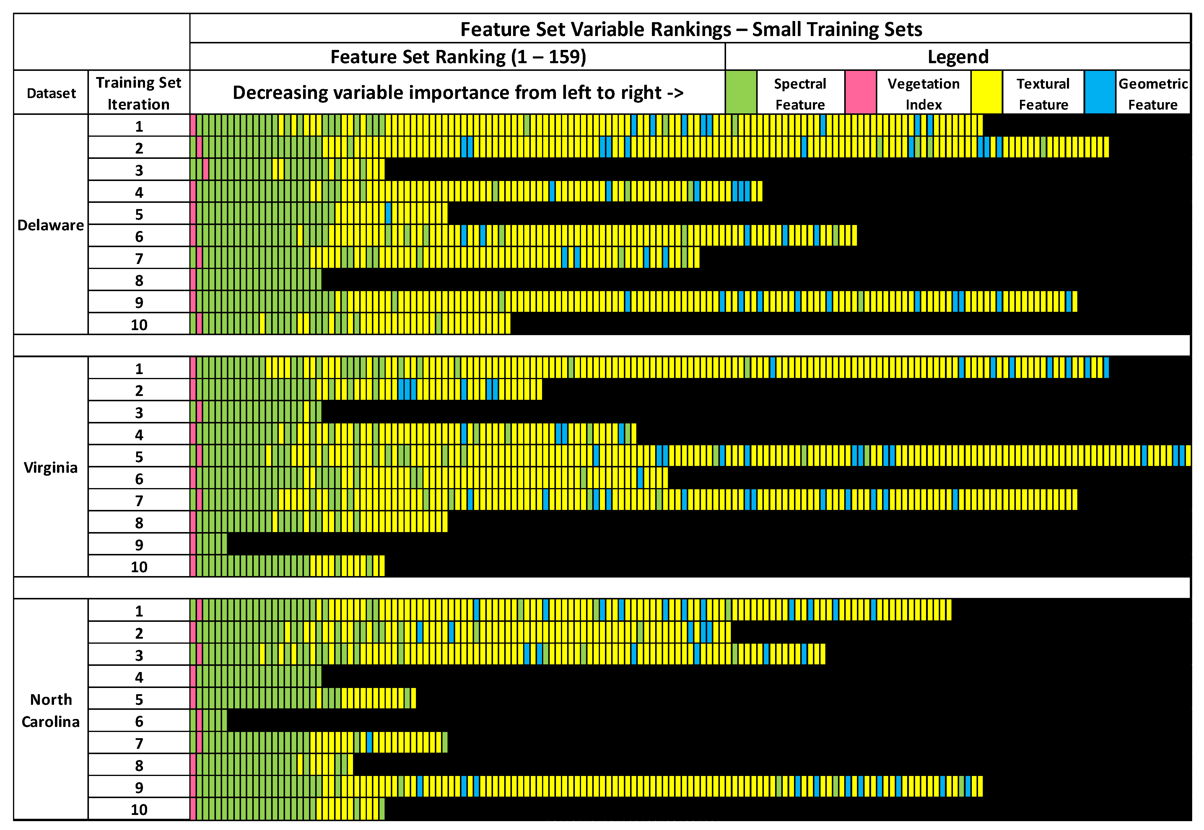
As seen in Figure 4, there was considerable variation in the feature selection results from the RFE process conducted on the small sample sets. Not only were there variations between the optimal feature sets of the sample sets acquired from different images, but also between sample sets acquired from the same image. Notably, none of the RFE-derived feature sets on the small training sets were identical. The number of optimal features between feature selection results of the Delaware small dataset ranged between 21 to 146. The feature sets of the small North Carolina dataset had the smallest range, between 6 to 126, while the small Virginia datasets had the largest range of features, between 6 to 159. Although there was minimal overlap in training samples between the small training sets, this wide variation in RFE results on training sets acquired from the same image was surprising.

The small Delaware feature sets also had the highest number of features that were included on all feature sets, at 21. Only six features were listed on all small Virginia and small North Carolina feature sets. Three features were found to be listed across all small training set feature sets: NDVI, max diff., and brightness. All feature sets contained at least one spectral variable. Textural features were included on 26 out of 30 (9 out 10 for Delaware, 9 out of 10 for Virginia, 8 out of 10 for North Carolina) of the small training set feature sets, while 18 out of 30 (7 out of 10 for Delaware, 6 out of 10 for Virginia, 5 out of 10 for North Carolina) small training set feature sets contained at least one geometric feature. Five feature sets were entirely comprised of spectral variables and did not include any geometric or textural features. Interestingly, only 32 out of 159 features were included in two-thirds or more of the small training set feature sets across all 3 images.

Regarding the feature selection results of the large training sets, variation between RFE-derived feature sets of training sets within the same image dataset, and between different image datasets was less than variations observed in the RFE-derived feature sets of the small training sets. This was expected, as the large training sets contain a considerable amount of overlap in terms of training image objects, at least between training sets of the same image dataset. Despite the high number of shared observations or training data overlap between the large training sample sets, there was still a notable amount of variation between training sets.

As seen in Figure 5, feature sets varied between training sets of the same image dataset, and between image datasets. Similar to the feature sets of the small training sets, no two RFE-derived feature sets of the large training sets were identical, which is surprising given the high overlap in training data between training sets acquired from the same image. However, the ranges of feature set size between different large training set feature sets were much smaller than the ranges of the small training set feature sets. The range of feature set sizes for the Delaware large training sets was between 16 to 86, while large training sets from the Virginia ranged between 41 to 86 features. The feature sets of the large North Carolina training sets had the smallest range of 46 to 81 features. Feature importance rankings were also more consistent between large training sets of the same image dataset, which is unsurprising given the overlap in image object samples between training sets. Most spectral features were consistently ranked higher in importance than textural or geometric features across all feature sets. All feature sets also included at least one spectral variable. All feature sets, except for one of the large Delaware training sets, included textural features. At least 1 geometric feature was included on 7 out of 10 of the large Delaware training sets, 9 out of 10 of the large Virginia training sets, and all of the large North Carolina feature sets.

The consistency of features across all training sets was also higher in the large training sets than the small training sets. In total, 16 features were included on all 10 large Delaware feature sets, while 38 features were included on all large Virginia feature sets. The large North Carolina feature sets had the most commonality, with 40 features that were included in all 10 datasets, including several textural and geometric features. Across all 30 training sets from all three image datasets, 16 spectral features were found on all datasets. Additionally, 47 out of 159 features were included on two-thirds or more of all large training set feature sets, a higher value than observed on the small training set feature sets. While the increase in feature set consistency between training sets acquired from the same image is likely due to the high overlap between the training sets, the increase in feature set consistency between the large training sets acquired from different images is surprising, and may suggest that larger training sets may be more useful for identifying image features that are consistently beneficial across multiple image datasets.

3.2. Classification Results—Small Training Sets

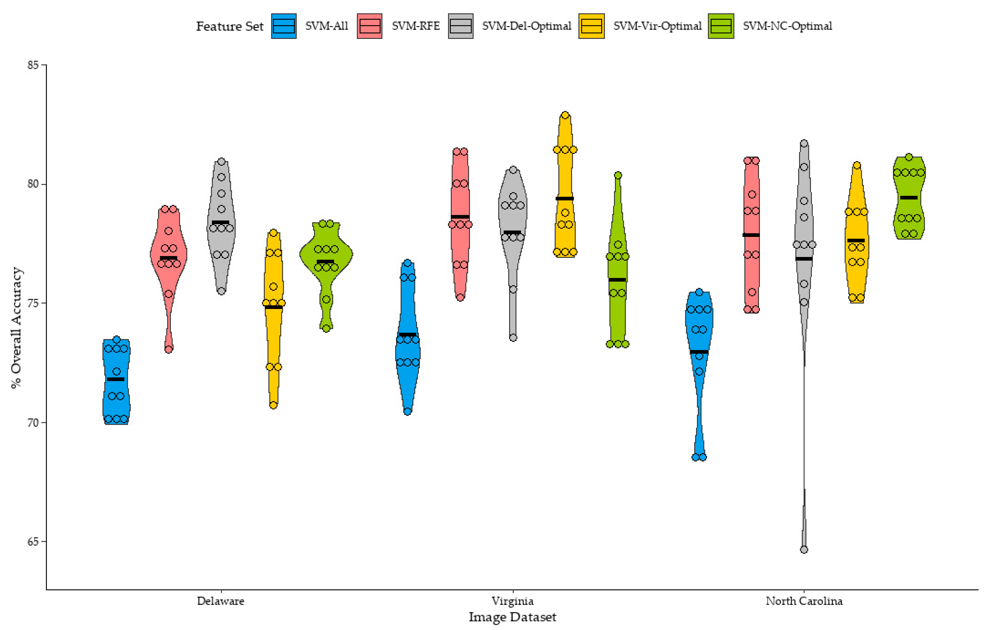
Figure 6 summarizes the distribution of overall accuracies of the classifications trained from the small sample sets. Classifications trained from the full sample set (SVM-All) produced the lowest mean overall accuracy for the Delaware, Virginia, and North Carolina datasets at 71.8%, 73.7%, and 72.9%, respectively. Classification accuracies for all training sets were consistently improved when the RFE process was individually applied to each training set (SVM-RFE). SVM-RFE mean classification accuracies improved by 5.1%, 4.9%, and 4.9% over SVM-All for classifications of the Delaware, Virginia, and North Carolina datasets, respectively. In general, feature selection was beneficial for improving classification accuracy for all classifications trained from the small sample sets.

Classifications trained using the feature set acquired from best SVM-RFE classification of the Delaware dataset (SVM-Del-Optimal) produced the highest overall mean accuracy of the Delaware dataset, at 78.3%, a 1.4% increase over the mean accuracy of the SVM-RFE classifications. While this is a relatively small increase, this result was unexpected, as the SVM-RFE process is thought to identify a feature set which optimizes the accuracy of each individual training set. It is interesting that a single feature set derived from an RFE process applied to a different training set was able to improve overall accuracy for some classifications. It should also be mentioned that, while the difference in means was small, the difference in means was found to be statistically significant.

Similarly, mean overall accuracies for the Virginia and North Carolina datasets were highest when the SVM-Vir-Optimal and SVM-NC-Optimal feature sets were applied to classifications of the Virginia, and North Carolina datasets, respectively. Mean overall accuracy of the SVM-Vir-Optimal classifications of the Virginia dataset was 0.7% higher than SVM-RFE classifications of the Virginia Dataset, although the difference in means between SVM-Vir-Optimal and SVM-RFE was found to be not statistically significant. However, while the difference in means was minimal, SVM-Vir-Optimal classifications provided higher overall accuracies over SVM-RFE classifications in six out of the ten replications.

For the North Carolina dataset, SVM-NC-Optimal classifications had a mean accuracy of 79.4%, 1.6% higher than the mean accuracy of the SVM-RFE classifications. The difference in means were also found to be statistically significant. Notably, one classification of the North Carolina dataset trained using the SVM-NC-Optimal feature set (

Table 6. Confusion matrix for an SVM-RFE classification of the North Carolina dataset trained from the small sample set (n = 108).

		Reference Data (No. of Objects)
		Developed	Exposed Soil	Forest	Grassland	Water	Wetlands	Total	User’s Accuracy
Classified Data (No. of Objects)	Developed	119	39	9	10	14	1	192	62.0%
	Exposed Soil	12	143	5	11	15	2	188	76.1%
	Forest	4	6	182	30	6	2	230	79.1%
	Grassland	5	20	22	219	0	0	266	82.3%
	Water	0	5	0	0	12	1	18	66.7%
	Wetlands	0	0	0	0	1	2	3	66.7%
	Total	140	213	218	270	48	8	897	Overall Accuracy: 75.5%
	Producer’s Accuracy	85.0%	67.1%	83.5%	81.1%	25.0%	25.0%

) had an overall accuracy of 80.4%, an improvement of 4.9% overall accuracy over the corresponding SVM-RFE classification using the same training set (

Table 7. Confusion matrix for an SVM-NC-Optimal classification of the North Carolina dataset trained from the small sample set (n = 108).

		Reference Data (No. of Objects)
		Developed	Exposed Soil	Forest	Grassland	Water	Wetlands	Total	User’s Accuracy
Classified Data (No. of Objects)	Developed	113	29	7	11	6	1	167	67.7%
	Exposed Soil	20	162	4	4	7	3	200	81.0%
	Forest	1	3	190	30	6	1	231	82.3%
	Grassland	6	17	17	225	0	0	265	84.9%
	Water	0	2	0	0	28	0	30	93.3%
	Wetlands	0	0	0	0	1	3	4	75.0%
	Total	140	213	218	270	48	8	897	Overall Accuracy: 80.4%
	Producer’s Accuracy	80.7%	76.1%	87.2%	83.3%	58.3%	37.5%

).

As indicated in Table 6 and Table 7, an example of improved performance of a classification trained using the NC-Optimal feature set was partially due to the RFE-SVM classifications’ relatively low user’s and producer’s accuracies of the water and wetlands classes. When the NC-Optimal feature set was used for this training set, user’s and producer’s accuracies of these classes were greatly improved, as well as the user’s and producer’s accuracies of the exposed soil, forest, and grassland classes. As these three classes comprise much of the composition of the test set, reduced classification error of these classes resulted in a substantial improvement in overall accuracy.

It should be mentioned that while the Del-Optimal, Virginia-Optimal, and NC-Optimal feature sets slightly improved the mean overall accuracy of the classifications of their respective image datasets, not all classifications saw an increase in overall accuracy. For example, two out of ten of the Delaware classifications saw a decrease in overall accuracy when the Del-Optimal feature set was used. When the Virginia-Optimal feature set was used for classifications of the Virginia dataset, one of the ten classifications saw a decrease in overall accuracy. Four out of ten SVM-NC-Optimal classifications saw a decrease in overall accuracy when compared to the SVM-RFE classifications of the North Carolina dataset. This suggests that a single optimal feature set may not be universally beneficial for improving classification accuracy for all training sample sets.

The SVM-Del-Optimal, SVM-Vir-Optimal, and SVM-NC-Optimal feature sets seemed to be beneficial to improving the mean accuracy of classification models of the same image dataset. However, when the optimal feature sets were transferred between images, mean classification accuracy tended to slightly decrease below the mean accuracy of the SVM-RFE classifications of each image dataset.

For example, the mean overall accuracy of the SVM-Del-Optimal and SVM-NC-Optimal classifications of the Virginia dataset were 77.9% and 75.9%, respectively, both lower than the mean overall accuracy of SVM-RFE and SVM-Vir-Optimal classifications of the Virginia dataset, at 78.6%, and 79.3%, respectively, although the difference in means between SVM-Del-Optimal and SVM-RFE classifications were found not to be significant. Classifications of the Delaware and North Carolina dataset followed a similar pattern. SVM-Vir-Optimal and SVM-NC-Optimal mean overall classification accuracies were lower than SVM-RFE or SVM-Del-Optimal when applied to classify the Delaware dataset. SVM-Vir-Optimal and SVM-Del-Optimal mean overall classification accuracies were also lower than SVM-RFE and SVM-NC-Optimal when applied to classify the North Carolina dataset.

Some mean classification accuracies were relatively close. For example, for the classifications of the Delaware dataset, the mean classification accuracy of SVM-RFE was 76.9% and SVM-NC-Optimal at 76.7%; the difference in means was found to be not statistically significant. While the mean accuracy of SVM-NC-Optimal was lower, performance was relatively similar to SVM-RFE for the Delaware dataset, but still lower than the mean overall accuracy of SVM-Del-Optimal at 78.4%. However, there were specific classifications which saw large differences in overall accuracy when trained from different feature sets. For example, an SVM-Del-Optimal classification of the North Carolina dataset saw a decrease in overall accuracy of 10.8% when compared to the corresponding SVM-RFE classification.

In general, for the classification’s trained from the small sample sets, optimal feature sets tended to slightly improve overall classification accuracy within the same image, but generally provided slightly lower overall accuracy when transferred to classifications of other images. However, these results were inconsistent between individual classifications, as some classifications saw a decrease in overall accuracy. Furthermore, the increase in mean overall accuracy over the SVM-RFE classifications for each dataset was relatively small. It should also be mentioned that overall accuracies of classifications which used an RFE-derived feature set, whether individually optimized (SVM-RFE), or one of the optimal feature sets, either from the same image or other images (SVM-Del-Optimal, SVM-Vir-Optimal, or SVM-NC-Optimal), were still typically higher than classifications trained using the full feature set (SVM-All).

Figure 7 provides an example visual representation of classifications of all three image datasets using different feature sets. There was notable classification error in all three image datasets between the water and developed classes, especially in the SVM-All classifications which used the full feature set.

3.3. Classification Results—Large Training Sets

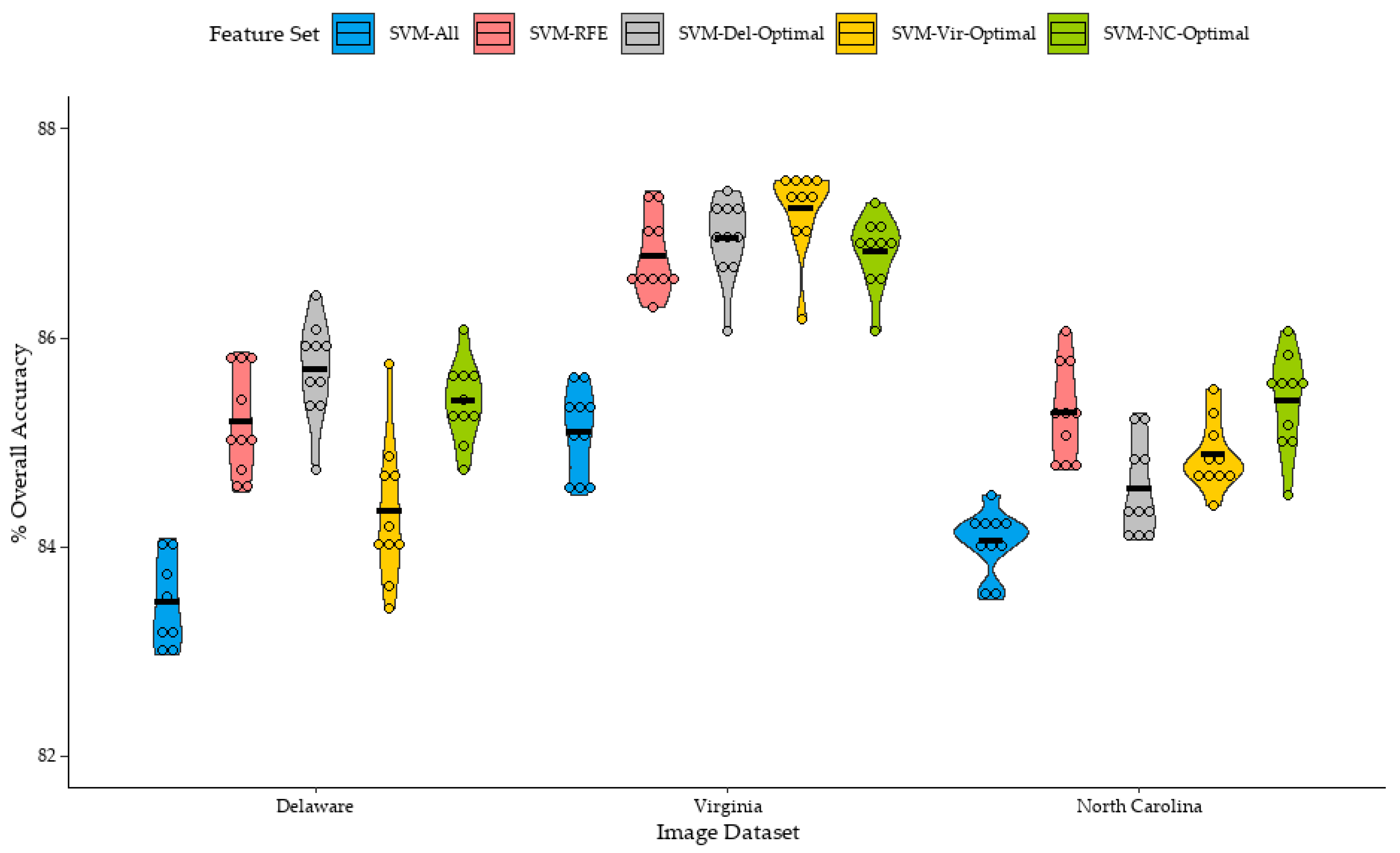
The distribution of overall accuracy of classifications trained from the large training sets are shown in Figure 8. Similar to the results of the small training set classifications, classifications which were trained from the full feature set (SVM-All) generally provided the lowest mean overall accuracies for the Delaware, Virginia, and North Carolina datasets, at 83.1%, 85.1%, and 84.0%, respectively. Feature selection was beneficial for improving classification accuracy, as the mean overall accuracy of the SVM-RFE classifications were 85.2%, 86.8%, and 85.3% for the Delaware, Virginia, and North Carolina datasets, respectively. It should be mentioned that improvement in classification accuracy using RFE-optimized feature sets over classifications using the full feature set was relatively smaller in the large training set classifications, compared to the small training set classifications. In congruence with observations from other studies employing the SVM classifier, this suggests that SVM may be sensitive to the Hughes effect, or the “curse of dimensionality” [50,51].

While the application of the Del-Optimal feature set to the large training set classifications of the Delaware dataset improved mean classification accuracy by 0.5% over SVM-RFE, the differences in means was not statistically significant. The largest improvement in classification accuracy of an SVM-Del-Optimal classification over an SVM-RFE classification of the Delaware datasets was 1.6%. However, similar to the small training sets, not all classifications saw an improvement in overall accuracy, as two classifications saw a decrease in overall accuracy of 0.3% and 0.6% when the SVM-Del-Optimal feature set was applied to the classifier.

The transference of the Del-Optimal feature set to large training set classifications of the Virginia and North Carolina datasets yielded mixed results. When the Del-Optimal feature set was applied to classifications of the North Carolina dataset, mean overall accuracy decreased by 0.7% compared to the mean accuracy of the SVM-RFE classifications, with the difference in means being found to be statistically significant. Nine out of ten classifications saw a decrease in accuracy; however, this decrease in accuracy was relatively small, with the largest decrease in overall accuracy at 1.8%. However, when the Del-Optimal feature set was applied to classifications of the Virginia dataset, mean overall accuracy slightly increased by 0.2%, and overall accuracy was comparable to SVM-RFE classifications of the Virginia dataset.

The Vir-Optimal feature set provided slightly higher mean overall accuracy for large sample set classifications of the Virginia dataset, at 86.9%, an increase of 0.5% over the SVM-RFE classification of the Virginia dataset, with the difference in means being statistically significant, while providing slightly lower mean overall accuracies for classifications of the Delaware and North Carolina datasets at 84.3%, and 84.9%, a decrease of 0.8% and 0.4%, respectively. Similar to the Del-Optimal dataset, not all Vir-Optimal datasets were beneficial for classifications of the Virginia dataset, as one classification saw a decrease in overall accuracy compared to the SVM-RFE classification, with the largest increase in overall accuracy being 1.0%.

Curiously, the NC-Optimal feature set provided slightly improved mean overall accuracy of the Delaware, Virginia, and North Carolina datasets and were largely comparable to the mean overall accuracies of each image dataset’s SVM-RFE classifications. However, similar to the Del-Optimal and Vir-Optimal feature sets, results tended to vary, with some classifications seeing an improvement in overall accuracy while others saw a decrease. Notably, the NC-Optimal feature set had the smallest increase in mean overall accuracy for the image dataset it was derived from, at 0.1%, at least when compared to the mean overall accuracy of the SVM-RFE classifications of the North Carolina dataset. It should be mentioned that the difference in means between SVM-RFE and SVM-NC-Optimal classifications of the North Carolina dataset were not statistically significant, which is expected given the extremely small difference in mean overall accuracy of the 10 replications.

A visual example set of classifications trained from the large training sets is depicted in Figure 9. In general, the highest performing classifications of each sample set looked visually good. However, there were visual differences between several classifications, some of which highlight errors within some of the maps. In the Delaware dataset, there was notable classification error between the exposed soil and wetlands classes in some coastal areas in the SVM-All and SVM-Vir-Optimal classifications. In this example, there was also notable classification error of the developed and exposed soil classes of the Virginia classification in the SVM-All and SVM-Del-Optimal classifications. The North Carolina classifications were visually similar, except for the SVM-All and SVM-Vir-Optimal classifications, which contained a high amount of error between the wetlands and exposed soil classes on the beachfront coastal area.

4. Discussion

Based upon the results presented in this analysis, I found that feature selection was generally beneficial for improving the accuracy of the SVM classifier, at least for producing object-based land cover classifications of Sentinel-2A MSI imagery. Feature selection was also found to be advantageous for SVM object-based land cover classification in studies by [4,5]. While feature selection was beneficial for classifications trained from both large and small training sets, the relative improvement in accuracy was greater in classifications trained from the small sample sets, which suggests that SVM may be sensitive to the Hughes effect [52,53]. While the results of this analysis suggest that SVM was sensitive to dimensionality, the sensitivity of SVM classifiers to the Hughes effect continues to be discussed within the remote sensing literature, as various works suggest that SVM is robust against the curse of dimensionality [54], while others suggest that SVM is sensitive to the dimensionality of the dataset [6,55].

I also found that feature selection results can not only widely vary between training sets of equivalent size and class composition acquired from similar remotely sensed datasets, but also between different training sets acquired from the same image, especially if the training set size is small. This is notable, as it suggests that feature selection results are in part tied to the specific training set; thus, different training sets may provide different insights on features, that may not be replicated with different training sample sets. Variability in feature selection results did decrease between the larger training sets [56,57], likely due to the fact that there was a high amount of overlap in image object samples between each training set acquired from the same image, although a surprising finding was that, in this case, the variability of feature selection results of training sets acquired from different images decreased as the size of the training set increased. This suggests that feature selection results may be more consistent within and between similar remotely sensed images when larger training sets are used. However, it should be mentioned that no two feature sets were identical across all of the large training sets. Thus, even when large training sets are used, specific feature selection results may not be replicated by other training sets of the same image, even if they contain a high overlap in training samples. On the other hand, it may be easier to identify consistently beneficial feature variables with larger training sets, as the variability in feature selection results decreased when larger training sets were used, even between training sets acquired from other images.

Despite the variation in feature selection results between different training sets, I found that specific feature selection results were largely transferable to other classification models of the same remotely sensed image, and even to classification models of other, similar, remotely sensed images. In this case, I found that feature sets generally transferred better to classification models of the same remotely sensed image, rather than to other images. However, the effects of feature set transference on classification accuracy were largely unpredictable for individual classifications. For some classifications, using a feature set derived from a high-performing classification model of the same remotely sensed image or a similar remotely sensed image resulted in a slight increase in accuracy, and for others, this resulted in a slight decrease in accuracy. In a few cases, feature set transference was highly detrimental to classification accuracy. Based upon the observed results on feature selection and classification accuracy in this analysis, several general recommendations for feature selection in future remote sensing analyses are provided:

For analysts attempting to gain insight on feature variables and importance rankings through reading prior similar analyses which report feature selection results, it should be kept in mind that the specific feature selection results in previous studies are largely dependent upon the training sample used, and the unique spectral and spatial properties of the dataset. As feature selection results can widely vary even on the same dataset, analyses should conduct their own feature selection processes within their analysis, rather than rely solely upon previous analyses’ insights.

Studies which incorporate feature selection and report on feature selection results should also note that feature sets and variable importance rankings may be specific to the training set and data used in the analysis and may or may not result in similar accuracies when reused for a different analysis, or even a different classification model of the same dataset. Thus, remote sensing analyses which report feature selection results should acknowledge that feature selection results are largely specific to the training data, or provide a disclaimer that specific feature sets may not be transferable to other classifications, even of the same remotely sensed dataset, as part of best practices.

Classification replication can be useful for providing more robust insights on beneficial features, as the analysis’ feature selection results would not be specific to a single classification model. Feature selection results between multiple classification models of the same image or multiple images can provide insights on patterns and commonalities in variable importance or feature rankings which may be a stronger indicator of generally beneficial feature variables.

Finally, the feature selection method itself should be emphasized over specific results. As feature selection has been found to be generally beneficial for a variety of machine learning classifiers, it is recommended that feature selection be included as part of the remote sensing classification workflow, when applicable.

It should be mentioned that this study had several limitations. This work investigated the transferability of feature selection results using a single feature selection method, and a single machine learning classifier, SVM, within a GEOBIA context. As other machine learning classifiers may be more sensitive or less sensitive to dataset dimensionality, this study could be expanded to explore other classification and feature selection methods. This study also used remotely sensed data which contained minimal temporal variation and was acquired from a single sensor. Furthermore, there was at least some overlap in image objects between both the large and small training sets; thus, each training set wasn’t entirely independent.

For future directions, feature set transferability should be investigated for pixel-based analyses as well. Investigations which incorporate additional machine learning classifiers and feature selection techniques would also be welcome. Investigating the transferability of feature sets between data from different sensors and temporally diverse datasets would also be an interesting expansion of this work.

5. Conclusions

This analysis investigated the transferability of feature selection results to other classification models of the same remotely sensed dataset trained from different sample sets, and to classification models of other, similar remotely sensed datasets. While feature selection was found to be generally beneficial for improving the accuracy of object-based SVM land cover classifications of Sentinel-2A multispectral imagery, considerable variation in feature selection results were found between different training sets of the same remotely sensed dataset, and between training sets from other remotely sensed datasets. While variability in feature selection results tended to decrease as the size of the training set was increased, there was still substantial variability between feature selection results, even when the training sets were mostly comprised of the same data. Thus, feature selection is highly dependent on the training data, and feature selection results are largely unique to a particular training set.

Transferring a feature set from a classification of one image to a classification of another, similar remotely sensed dataset, or to other classifications of the same remotely sensed dataset provided inconsistent results. This inconsistency reduces the utility of transferring feature selection derived feature sets from one classification to another, as the feature set does not reliably generalize to other training sets and classifications.

Consequently, only general insights should be taken from feature selection results in similar remotely sensed analyses, as it can be difficult to know if a specific feature set, when transferred, will be beneficial or detrimental to a different classification model and training set. Furthermore, remote sensing analyses should acknowledge that feature selection results are largely data specific, may not be replicated in similar analyses, and may not transfer to other classifications, as part of best practices when reporting feature selection results or variable importance rankings. Feature selection and feature set optimization processes should be individually conducted for each classification model as part of the classification workflow to determine an optimal feature set for the training set and classifier employed in the analysis.

References

1. Ma, L.; Fu, T.; Blaschke, T.; Li, M.; Tiede, D.; Zhou, Z.; Ma, X.; Chen, D. Evaluation of Feature Selection Methods for Object-Based Land Cover Mapping of Unmanned Aerial Vehicle Imagery Using Random Forest and Support Vector Machine Classifiers. IJGI 2017, 6, 51. [Google Scholar] [CrossRef] [Green Version]
2. Maxwell, A.E.; Warner, T.A.; Fang, F. Implementation of Machine-Learning Classification in Remote Sensing: An Applied Review. Int. J. Remote Sens. 2018, 39, 2784–2817. [Google Scholar] [CrossRef] [Green Version]
3. Zhou, Y.; Zhang, R.; Wang, S.; Wang, F. Feature Selection Method Based on High-Resolution Remote Sensing Images and the Effect of Sensitive Features on Classification Accuracy. Sensors 2018, 18, 2013. [Google Scholar] [CrossRef] [PubMed] [Green Version]
4. Kiala, Z.; Mutanga, O.; Odindi, J.; Peerbhay, K. Feature Selection on Sentinel-2 Multispectral Imagery for Mapping a Landscape Infested by Parthenium Weed. Remote Sens. 2019, 11, 1892. [Google Scholar] [CrossRef] [Green Version]
5. Stromann, O.; Nascetti, A.; Yousif, O.; Ban, Y. Dimensionality Reduction and Feature Selection for Object-Based Land Cover Classification Based on Sentinel-1 and Sentinel-2 Time Series Using Google Earth Engine. Remote Sens. 2019, 12, 76. [Google Scholar] [CrossRef] [Green Version]
6. Pal, M.; Foody, G.M. Feature Selection for Classification of Hyperspectral Data by SVM. IEEE Trans. Geosci. Remote Sens. 2010, 48, 2297–2307. [Google Scholar] [CrossRef] [Green Version]
7. Jiang, X.; Tang, L.; Wang, C.; Wang, C. Spectral Characteristics and Feature Selection of Hyperspectral Remote Sensing Data. Int. J. Remote Sens. 2004, 25, 51–59. [Google Scholar] [CrossRef]
8. Kganyago, M.; Odindi, J.; Adjorlolo, C.; Mhangara, P. Selecting a Subset of Spectral Bands for Mapping Invasive Alien Plants: A Case of Discriminating Parthenium Hysterophorus Using Field Spectroscopy Data. Int. J. Remote Sens. 2017, 38, 5608–5625. [Google Scholar] [CrossRef]
9. Jawak, S.D.; Wankhede, S.F.; Luis, A.J.; Balakrishna, K. Effect of Image-Processing Routines on Geographic Object-Based Image Analysis for Mapping Glacier Surface Facies from Svalbard and the Himalayas. Remote Sens. 2022, 14, 4403. [Google Scholar] [CrossRef]
10. Wei, C.; Guo, B.; Fan, Y.; Zang, W.; Ji, J. The Change Pattern and Its Dominant Driving Factors of Wetlands in the Yellow River Delta Based on Sentinel-2 Images. Remote Sens. 2022, 14, 4388. [Google Scholar] [CrossRef]
11. Blaschke, T. Object Based Image Analysis for Remote Sensing. ISPRS J. Photogramm. Remote Sens. 2010, 65, 2–16. [Google Scholar] [CrossRef] [Green Version]
12. Demarchi, L.; Kania, A.; Ciężkowski, W.; Piórkowski, H.; Oświecimska-Piasko, Z.; Chormański, J. Recursive Feature Elimination and Random Forest Classification of Natura 2000 Grasslands in Lowland River Valleys of Poland Based on Airborne Hyperspectral and LiDAR Data Fusion. Remote Sens. 2020, 12, 1842. [Google Scholar] [CrossRef]
13. Fu, B.; He, X.; Yao, H.; Liang, Y.; Deng, T.; He, H.; Fan, D.; Lan, G.; He, W. Comparison of RFE-DL and Stacking Ensemble Learning Algorithms for Classifying Mangrove Species on UAV Multispectral Images. Int. J. Appl. Earth Obs. Geoinf. 2022, 112, 102890. [Google Scholar] [CrossRef]
14. Sesnie, S.; Eagleston, H.; Johnson, L.; Yurcich, E. In-Situ and Remote Sensing Platforms for Mapping Fine-Fuels and Fuel-Types in Sonoran Semi-Desert Grasslands. Remote Sens. 2018, 10, 1358. [Google Scholar] [CrossRef] [Green Version]
15. Zhou, Y.; Tian, S.; Chen, J.; Liu, Y.; Li, C. Research on Classification of Open-Pit Mineral Exploiting Information Based on OOB RFE Feature Optimization. Sensors 2022, 22, 1948. [Google Scholar] [CrossRef]
16. Zhang, N.; Chen, M.; Yang, F.; Yang, C.; Yang, P.; Gao, Y.; Shang, Y.; Peng, D. Forest Height Mapping Using Feature Selection and Machine Learning by Integrating Multi-Source Satellite Data in Baoding City, North China. Remote Sens. 2022, 14, 4434. [Google Scholar] [CrossRef]
17. Zhang, R.; Ma, J. Feature Selection for Hyperspectral Data Based on Recursive Support Vector Machines. Int. J. Remote Sens. 2009, 30, 3669–3677. [Google Scholar] [CrossRef]
18. Wei, P.; Zhu, W.; Zhao, Y.; Fang, P.; Zhang, X.; Yan, N.; Zhao, H. Extraction of Kenyan Grassland Information Using PROBA-V Based on RFE-RF Algorithm. Remote Sens. 2021, 13, 4762. [Google Scholar] [CrossRef]
19. Ebrahimi-Khusfi, Z.; Nafarzadegan, A.R.; Dargahian, F. Predicting the Number of Dusty Days around the Desert Wetlands in Southeastern Iran Using Feature Selection and Machine Learning Techniques. Ecol. Indic. 2021, 125, 107499. [Google Scholar] [CrossRef]
20. Hong, F.; Kong, Y. Random Forest Fusion Classification of Remote Sensing PolSAR and Optical Image Based on LASSO and IM Factor. In Proceedings of the 2021 IEEE International Geoscience and Remote Sensing Symposium IGARSS, Brussels, Belgium, 11 July 2021; IEEE: Piscataway, NJ, USA; pp. 5048–5051. [Google Scholar]
21. Commission for Environmental Cooperation. Ecological Regions of North America: Towards a Common Perspective; Commission for Environmental Cooperation: Montreal, QC, Canada, 1997; ISBN 2-922305-18-X. [Google Scholar]
22. Blaschke, T.; Hay, G.J.; Kelly, M.; Lang, S.; Hofmann, P.; Addink, E.; Queiroz Feitosa, R.; van der Meer, F.; van der Werff, H.; van Coillie, F.; et al. Geographic Object-Based Image Analysis—Towards a New Paradigm. ISPRS J. Photogramm. Remote Sens. 2014, 87, 180–191. [Google Scholar] [CrossRef]
23. Phiri, D.; Simwanda, M.; Salekin, S.; Nyirenda, V.; Murayama, Y.; Ranagalage, M. Sentinel-2 Data for Land Cover/Use Mapping: A Review. Remote Sens. 2020, 12, 2291. [Google Scholar] [CrossRef]
24. Trimble. eCognition Developer, version 9.3; Trimble Germany GmBH: Munich, Germany, 2021. [Google Scholar]
25. Drăguţ, L.; Csillik, O.; Eisank, C.; Tiede, D. Automated Parameterisation for Multi-Scale Image Segmentation on Multiple Layers. ISPRS J. Photogramm. Remote Sens. 2014, 88, 119–127. [Google Scholar] [CrossRef] [PubMed] [Green Version]
26. Bialas, J.; Oommen, T.; Rebbapragada, U.; Levin, E. Object-Based Classification of Earthquake Damage from High-Resolution Optical Imagery Using Machine Learning. J. Appl. Remote Sens. 2016, 10, 036025. [Google Scholar] [CrossRef] [Green Version]
27. Kuc, G.; Chormański, J. SENTINEL-2 Imagery for Mapping and Monitoring Imperviousness in Urban Areas. Int. Arch. Photogramm. Remote Sens. Spat. Inf. Sci. 2019, XLII-1/W2, 43–47. [Google Scholar] [CrossRef] [Green Version]
28. Misra, G.; Cawkwell, F.; Wingler, A. Status of Phenological Research Using Sentinel-2 Data: A Review. Remote Sens. 2020, 12, 2760. [Google Scholar] [CrossRef]
29. Morell-Monzó, S.; Estornell, J.; Sebastiá-Frasquet, M.-T. Comparison of Sentinel-2 and High-Resolution Imagery for Mapping Land Abandonment in Fragmented Areas. Remote Sens. 2020, 12, 2062. [Google Scholar] [CrossRef]
30. Frampton, W.J.; Dash, J.; Watmough, G.; Milton, E.J. Evaluating the Capabilities of Sentinel-2 for Quantitative Estimation of Biophysical Variables in Vegetation. ISPRS J. Photogramm. Remote Sens. 2013, 82, 83–92. [Google Scholar] [CrossRef] [Green Version]
31. Chaves, M.E.D.; Picoli, M.C.A.; Sanches, I.D. Recent Applications of Landsat 8/OLI and Sentinel-2/MSI for Land Use and Land Cover Mapping: A Systematic Review. Remote Sens. 2020, 12, 3062. [Google Scholar] [CrossRef]
32. Kim, M.; Warner, T.A.; Madden, M.; Atkinson, D.S. Multi-Scale GEOBIA with Very High Spatial Resolution Digital Aerial Imagery: Scale, Texture and Image Objects. Int. J. Remote Sens. 2011, 32, 2825–2850. [Google Scholar] [CrossRef]
33. Kim, M.; Madden, M.; Xu, B. GEOBIA Vegetation Mapping in Great Smoky Mountains National Park with Spectral and Non-Spectral Ancillary Information. Photogramm. Eng. Remote Sens. 2010, 76, 137–149. [Google Scholar] [CrossRef]
34. Warner, T. Kernel-Based Texture in Remote Sensing Image Classification: Kernel-Based Texture in Remote Sensing. Geogr. Compass 2011, 5, 781–798. [Google Scholar] [CrossRef]
35. Haralick, R.M.; Shanmugam, K.; Dinstein, I. Textural Features for Image Classification. IEEE Trans. Syst. Man Cybern. 1973, SMC-3, 610–621. [Google Scholar] [CrossRef] [Green Version]
36. Iqbal, N.; Mumtaz, R.; Shafi, U.; Zaidi, S.M.H. Gray Level Co-Occurrence Matrix (GLCM) Texture Based Crop Classification Using Low Altitude Remote Sensing Platforms. PeerJ. Comput. Sci. 2021, 7, e536. [Google Scholar] [CrossRef]
37. Karlson, M.; Reese, H.; Ostwald, M. Tree Crown Mapping in Managed Woodlands (Parklands) of Semi-Arid West Africa Using WorldView-2 Imagery and Geographic Object Based Image Analysis. Sensors 2014, 14, 22643–22669. [Google Scholar] [CrossRef] [PubMed] [Green Version]
38. Kucharczyk, M.; Hay, G.J.; Ghaffarian, S.; Hugenholtz, C.H. Geographic Object-Based Image Analysis: A Primer and Future Directions. Remote Sens. 2020, 12, 2012. [Google Scholar] [CrossRef]
39. Kuhn, M. Building Predictive Models in R Using the caret Package. J. Stat. Softw. 2008, 28, 1–26. [Google Scholar] [CrossRef] [Green Version]
40. Ramezan, C.A.; Warner, T.A.; Maxwell, A.E. Evaluation of Sampling and Cross-Validation Tuning Strategies for Regional-Scale Machine Learning Classification. Remote Sens. 2019, 11, 185. [Google Scholar] [CrossRef] [Green Version]
41. Cortes, C.; Vapnik, V. Support-Vector Networks. Mach. Learn. 1995, 20, 273–297. [Google Scholar] [CrossRef]
42. Pal, M. Kernel Methods in Remote Sensing: A Review. ISH J. Hydraul. Eng. 2009, 15, 194–215. [Google Scholar] [CrossRef]
43. Mountrakis, G.; Im, J.; Ogole, C. Support Vector Machines in Remote Sensing: A Review. ISPRS J. Photogramm. Remote Sens. 2011, 66, 247–259. [Google Scholar] [CrossRef]
44. Breiman, L. Random Forests. Mach. Learn. 2001, 45, 5–32. [Google Scholar] [CrossRef] [Green Version]
45. Kohonen, T. An Introduction to Neural Computing. Neural Netw. 1998, 1, 3–17. [Google Scholar] [CrossRef]
46. Chen, L.; Cheng, X. Classification of High-Resolution Remotely Sensed Images Based on Random Forests. J. Softw. Eng. 2016, 10, 318–327. [Google Scholar] [CrossRef]
47. Ramo, R.; Chuvieco, E. Developing a Random Forest Algorithm for MODIS Global Burned Area Classification. Remote Sens. 2017, 9, 1193. [Google Scholar] [CrossRef] [Green Version]
48. Maxwell, A.E.; Strager, M.P.; Warner, T.A.; Ramezan, C.A.; Morgan, A.N.; Pauley, C.E. Large-Area, High Spatial Resolution Land Cover Mapping Using Random Forests, GEOBIA, and NAIP Orthophotography: Findings and Recommendations. Remote Sens. 2019, 11, 1409. [Google Scholar] [CrossRef] [Green Version]
49. Paola, J.D.; Schowengerdt, R.A. A Review and Analysis of Backpropagation Neural Networks for Classification of Remotely-Sensed Multi-Spectral Imagery. Int. J. Remote Sens. 1995, 16, 3033–3058. [Google Scholar] [CrossRef]
50. Golhani, K.; Balasundram, S.K.; Vadamalai, G.; Pradhan, B. A Review of Neural Networks in Plant Disease Detection Using Hyperspectral Data. Inf. Processing Agric. 2018, 5, 354–371. [Google Scholar] [CrossRef]
51. Student The Probable Error of a Mean. Biometrika 1908, 1–25. Available online: https://www.jstor.org/stable/2331554 (accessed on 17 September 2022).
52. Hughes, G. On the Mean Accuracy of Statistical Pattern Recognizers. IEEE Trans. Inform. Theory 1968, 14, 55–63. [Google Scholar] [CrossRef] [Green Version]
53. Thenkabail, P.; Gumma, M.K.; Teluguntla, P.; Ahmed, M.I. Hyperspectral Remote Sensing of Vegetation and Agricultural Crops. Photogramm. Eng. Remote Sens. 2014, 80, 697–723. [Google Scholar]
54. Salimi, A.; Ziaii, M.; Amiri, A.; Hosseinjani Zadeh, M.; Karimpouli, S.; Moradkhani, M. Using a Feature Subset Selection Method and Support Vector Machine to Address Curse of Dimensionality and Redundancy in Hyperion Hyperspectral Data Classification. Egypt J. Remote Sens. Space Sci. 2018, 21, 27–36. [Google Scholar] [CrossRef]
55. Pal, M. Support Vector Machine-based Feature Selection for Land Cover Classification: A Case Study with DAIS Hyperspectral Data. Int. J. Remote Sens. 2006, 27, 2877–2894. [Google Scholar] [CrossRef]
56. Gong, P.; Liu, H.; Zhang, M.; Li, C.; Wang, J.; Huang, H.; Clinton, N.; Ji, L.; Li, W.; Bai, Y.; et al. Stable Classification with Limited Sample: Transferring a 30-m Resolution Sample Set Collected in 2015 to Mapping 10-m Resolution Global Land Cover in 2017. Sci. Bull. 2019, 64, 370–373. [Google Scholar] [CrossRef] [Green Version]
57. Li, C.; Wang, J.; Wang, L.; Hu, L.; Gong, P. Comparison of Classification Algorithms and Training Sample Sizes in Urban Land Classification with Landsat Thematic Mapper Imagery. Remote Sens. 2014, 6, 964–983. [Google Scholar] [CrossRef]
Figure 1. Study area and Sentinel-2 false color composites displaying bands NIR, red, and green, as RGB. (a) Study area locations. (b) Delaware image dataset. (c) Virginia image dataset. (d) North Carolina image dataset.
Remotesensing 14 06218 g001
Figure 2. Overview of the experimental workflow.
Remotesensing 14 06218 g002
Figure 3. Recursive feature elimination process workflow.
Remotesensing 14 06218 g003
Figure 4. RFE-derived feature set rankings for small Delaware, Virginia, and North Carolina training sets. Each row indicates the features that were found to be optimal for the training set by the RFE process. Each cell indicates the type of feature that was included in the RFE-derived feature set, ranked in decreasing importance to the accuracy of the classification from left to right.
Remotesensing 14 06218 g004
Figure 5. RFE-derived feature set rankings for large Delaware, Virginia, and North Carolina training sets. Each row indicates the features that were found to be optimal for the training set by the RFE process. Each cell indicates the type of feature that was included in the RFE-derived feature set, ranked in decreasing importance to the accuracy of the classification from left to right.
Remotesensing 14 06218 g005
Figure 6. Distribution of overall accuracies of classifications trained from small sample sets. The black horizontal bar indicates the mean overall accuracy for each classification method, while the circles approximate individual overall accuracy values of classifications.
Remotesensing 14 06218 g006
Figure 7. Example set of land cover classifications of the Delaware, Virginia, and North Carolina datasets trained from the small training sets using a variety of feature sets, including the full feature set (SVM-All), SVM-RFE, SVM-Del-Optimal, SVM-Vir-Optimal, and SVM-NC-Optimal. The Sentinel-2A imagery is displayed as a false-color composite with bands 8 (NIR), 4 (red), and 3 (green) depicted as RGB.
Remotesensing 14 06218 g007
Figure 8. Distribution of overall accuracies of classifications trained from large sample sets. The black horizontal bar indicates the mean overall accuracy for each classification method while the circles approximate individual overall accuracy values of classifications.
Remotesensing 14 06218 g008
Figure 9. Example set of land cover classifications of the Delaware, Virginia, and North Carolina datasets trained from the large training sets using a variety of feature sets, including the full feature set (SVM-All), SVM-RFE, SVM-Del-Optimal, SVM-Vir-Optimal, and SVM-NC-Optimal. The Sentinel-2A imagery is displayed as a false-color composite with bands 8 (NIR), 4 (red), and 3 (green) depicted as RGB.
Remotesensing 14 06218 g009