Editorial

Recent Advances in Modelling Geodetic Time Series and Applications for Earth Science and Environmental Monitoring

1
School of Civil and Surveying & Mapping Engineering, Jiangxi University of Science and Technology, Ganzhou 341000, China
2
Physikalisch-Meteorologisches Observatorium Davos/World Radiation Center (PMOD/WRC), CH-7260 Davos, Switzerland
3
Institute Dom Luiz (IDL), University of Beira Interior, 6201-001 Covilhã, Portugal
4
GNSS Research Center, Wuhan University, Wuhan 430079, China
5
Institute for Meterology and Climatology, Leibniz Universität Hannover, Herrenhäuserstr. 2, 30419 Hannover, Germany
6
College of Geodesy and Geomatics, Shandong University of Science and Technology, Qingdao 266590, China
*
Author to whom correspondence should be addressed.
Remote Sens. 2022, 14(23), 6164; https://doi.org/10.3390/rs14236164
Submission received: 21 November 2022 / Revised: 24 November 2022 / Accepted: 28 November 2022 / Published: 5 December 2022

Abstract

:
Geodesy is the science of accurately measuring the topography of the earth (geometric shape and size), its orientation in space, and its gravity field. With the advances in our knowledge and technology, this scientific field has extended to the understanding of geodynamical phenomena such as crustal motion, tides, and polar motion. This Special Issue is dedicated to the recent advances in modelling geodetic time series recorded using various instruments. Due to the stochastic noise properties inherent in each of the time series, careful modelling is necessary in order to extract accurate geophysical information with realistic associated uncertainties (statistically sufficient). The analyzed data have been recorded with various space missions or ground-based instruments. It is impossible to be comprehensive in the vast and dynamic field that is Geodesy, particularly so-called “Environmental Geodesy”, which intends to understand the Earth’s geodynamics by monitoring any changes in our environment. This field has gained much attention in the past two decades due to the need by the international community to understand how climate change modifies our environment. Therefore, this Special Issue collects some articles which emphasize the recent development of specific algorithms or methodologies to study particular natural phenomena related to the geodynamics of the earth’s crust and climate change.

1. Introduction: A Short Historical Review on Geodesy and the Space Geodesy Era

Geodesy has a long history which goes back to surveyors in ancient Egypt, where a rope stretcher would use simple geometry to re-establish boundaries after the annual floods of the Nile River. Basic Geodesy was also used by the Egyptians, known for their advanced skills in early surveying techniques, in establishing the squareness and north–south orientation of the Great Pyramid of Giza (built c. 2700 BC) [1]. Through the ages, various monuments have been built thanks to early surveying techniques (e.g., Stonehenge, 2500 BC [2]) or to make rough measurements delimiting the regions within empires (e.g., Roman Empire). Different techniques have been developed across the ages improving surveying observations. More recently, Geodesy has undergone a huge revolution, starting in the 1950s with the development of electronic distance measurement equipment. These instruments saved the need for days or weeks of chain observations by directly measuring between points kilometers apart. A few years later, the first satellite positioning system was created: the US Navy TRANSIT system [3]. The first successful launch took place in 1959. This was the beginning of the “Space Geodesy” era. The concept of space Geodesy, with a constellation of satellites dedicated to providing the position of a rover anywhere and anytime on the surface of the earth with high accuracy, dates back to the early 1960s as a military concept developed independently by the USA and the USSR under the famous names Global Positioning System (GPS) and the Globalnaya Navigatsionnaya Sputnikovaya Sistema (GLONASS), respectively. Since opening these military systems to the public in the mid-1990s, this technology has generated a multi-billion-dollar market relying on location-based services [4]. These services require an accurate and timely estimate of a user’s position at all times, in all environments and across all acquisition modes. This global coverage has been improved by increasing the number of satellite constellations. As of September 2020, GPS, GLONASS, China’s BeiDou navigation system, and the European Union’s Galileo are fully operational constellations [5]. Additionally, the Japan’s Quasi-Zenith Satellite System (QZSS) is an augmented satellite system, with a focus on Japan and the Asia–Oceania region. Besides launching new satellites, services are developed based on a network of GNSS reference stations to provide specific correction values to the user in real time or for post-processing, for example SAPOS in Germany [6]. All these constellations, used to accurately position a rover or a permanently fixed receiver (normally known as CORS—Continuously Operating Reference Station), are gathered under the general name Global Navigation Satellite Systems (GNSS). This Special Issue is dedicated to several applications focused on the analysis of the time-series obtained from CORS observations with a focus on environmental applications but also for deformation monitoring within the context of early-warning systems. Early-warning systems are an adaptive measure for climate change, using integrated communication systems to help communities prepare for hazardous climate-related events.

2. Environmental Geodesy: Continuously Monitoring the Geodynamics of the Earth and the Effects of Climate Change, and Detecting Natural Hazards

Many satellite Geodesy techniques are used, such as GPS, the Gravity Recovery and Climate Experiment (GRACE), and Interferometric Synthetic Aperture Radar (InSAR), to monitor the geodynamics of the earth (e.g., crustal deformation due to earthquakes, impact of droughts, and the study of tectonic plates) and the modifications in our environment due to climate changes (e.g., monitoring sea level and melting of the ice sheet). These various examples define so-called “Environmental Geodesy” [7]. In the following section, we introduce and discuss several areas to which some articles included in this Special Issue have contributed.

2.1. Continuously Monitoring Crustal Deformation and Detecting Natural Hazards with GNSS and InSAR

Large networks of permanent GNSS stations set up around the world provide spatial and temporal information on surface deformation processes, including plate motion [8], crustal deformation due to earthquakes (i.e., pre-, co-, and post-seismic offsets [9]), tectonic strain, glacial isostatic adjustment [10], surface loading [11], and tropospheric modeling with the determination of water vapor [12]. At the moment, more than 15,000 permanent GNSS stations are fully operational and provide daily positions with sub-centimeter-level accuracy [13].
The antennae of permanent GNSS stations have been installed on a large variety of monuments. Generally, the metadata file (or log file) associated with each station provides a description of the monument, often referred to as mast, pillar, roof top, tower, or tripod [14]. Several studies [15,16,17] have classified all monument types into four categories: concrete piers, deep-drilled brace monuments, shallow-drilled brace monuments, and roof tops/chimneys. A concrete pier is a pillar attached deeply into the ground that can reach several meters below the surface. A deep-drilled brace monument is a braced monument where four or five pipes are installed and cemented into inclined boreholes with the antenna attached at ~1 m above the surface. The pipes are also attached deeply below the surface (up to ~10 m). A shallow-drilled brace monument refers to the type of monument which is attached to the surface (<1m-deep) using a hand-driller. The fourth category encompasses antennas installed on the top of buildings, sometimes using a mast attached to a wall or with a concrete support. One of the open questions in Geodesy is whether there is a relationship between the type of monument and the stochastic noise properties of the recorded GNSS daily position time series. Several studies have concluded that the spatial distribution of the monument supersedes the type of monument in the selection of the noise model for the global, not regionally filtered, GNSS time series. Herring et al. [15] warned about the spatial distribution across North America when studying the relationship between a type of monument and the stochastic noise model. Williams et al. [18] restricted their study to a small area to determine the influence of the various types of monuments. Beavan [19] concluded that monument noise is not the dominant factor in the stochastic noise properties of the GPS time series and He et al. [17] corroborated these results.
Moreover, analysis of the variations in the position over time provides important information about various geophysical processes. Examples are the estimation of the motion of tectonic plates, the deflation/inflation event of volcanos, the offsets produced by earthquakes, the vertical land motion of continents induced by post-glacial rebound, the movement of glaciers, and the estimation of particular transient signals (e.g., slow slip events and post-seismic transients [20]) which are sometimes precursors of natural hazards (e.g., landslides [21]). For example, large landslides in steep alpine slopes are a considerable threat to vulnerable communities and infrastructures. Their destructive power is related to their potential to undergo rapid accelerations and evolve into catastrophic rock avalanches, which expose valley bottoms to exceptional risks [22]. An accurate characterization of these phenomena requires a thorough understanding of the predisposing geological factors, controlling factors, and failure mechanism. Geotechnical surveys together with GNSS permanent stations, when available, allow detecting particular transient signals in order to trigger early-warning systems. However, this is heavily constrained by logistical and/or economical limitations, owing to the typically vast, difficult, and remote terrains. Therefore, recent studies have used the Interferometric Synthetic Aperture Radar (InSAR) technology together with GNSS [23].
Differential radar interferometry is a well-established active remote sensing technique that exploits the phase shift of the back-scattered electromagnetic wave between two or more coherent acquisitions. The recorded scene is arranged in a two-dimensional image and partitioned into pixels [24]. Knowing the approximate 3D geometry of the slope surface deformation is essential for correcting InSAR-derived displacements, which can be carried out with GNSS stations near the area of interest if the data are available, such as in Huang’s [25] and Guo’s [26] studies.
Within geodetic time series, surface deformation processes can only be modeled to a certain degree and estimated with the correct functional and stochastic models when studying geophysical processes, such as tectonic rates and seasonal signal [27,28,29]. Among all the residual errors in the GNSS time series, unmodeled pseudo-periodic signals cause spurious periodicities and even induce biases in estimating true periodic seasonal variations [30]. The causes of these residual errors may originate from mismodeled geophysical phenomena (e.g., non-deterministic seasonal signal [31]). In general, the contribution to seasonal variations in the estimated site positions can be grouped into several categories: gravitational excitation (displacements due to solid earth, ocean tides, and atmospheric tides) [32] and various residual errors which could also generate apparent seasonal variations (e.g., draconitic signals resulting from mismodelling satellite orbits) [33,34].

2.2. Monitoring with Terrestrial Laser Scanners and GNSS

Monitoring high-mountain areas is mandatory within the context of climate change and the expansion of areas of urban settlement. Here, not only landslide identification plays an important role in risk assessment but also prediction for early-warning systems. The latter necessitates high-quality datasets that are both spatially and temporally detailed. GNSS and terrestrial laser scanners (TLS) are economically attractive and contact-less systems which are widely used within this context [35]. The prediction of deformation remains an active research field where machine learning techniques will play an increasing role. In this Special Issue, Zhu et al. [36] proposed an innovative method combining wireless sensors including a reservoir water level gauge, rainfall gauge, and GNSS. Their method, based on double exponential smoothing and the particle swarm optimization–extreme learning machine, is a novel artificial neural network architecture to forecast landslide displacement, and was applied successfully for the Baijiabao landslide in China. Similarly, Huang et al. [37] used a salp-swarm-algorithm-optimized temporal convolutional network to predict the periodic displacement of the Muyubao landslide considering the response relationship between periodic displacement recorded by a GPS monitoring system, rainfall, and reservoir water. These improvements show the potential of combining datasets from different sources and should support the increasing needs for predicting deformation based on TLS observations, potentially coupled with GNSS observations. Here, mathematical approximation of the surface, as proposed in Kermarrec et al. [38] with locally refined B-splines, will strongly mitigate the problems linked with the huge data size.

2.3. Monitoring Sea-Level Rise for Coastal Resilience

One of the major impacts of climate change is a rise in the global sea level caused by the melting of glaciers and land-based ice caps, as well as a smaller increase from expansion due to the higher temperature of the water itself. The scientific community has estimated that sea-level rise (SLR) has reached almost ~8 cm globally since 1992 [39] and amounted to between 0.3 and 0.9 m by the end of the century [40]. Coastal cities around the world have begun to grapple with the risks of sea-level rise. Some of them face the threats of tidal flooding, non-tropical-storm flooding, and tropical cyclone storm surge. Therefore, governments and local authorities issue a strategic plan for climate resilience and adaption in order to face potential natural hazards with the associated economical and human costs [41].
Using geodetic observations, several studies [42,43] have estimated the relative sea-level rise using tide gauges (TGs). However, TGs cannot measure the absolute sea-level change, but the height of the sea surface relative to crustal reference points that may move with tectonic activity or local subsidence. In other words, the TG observations are biased by local and regional processes that are linear or non-linear over a multi-decade timescale. Linear processes include glacial isostatic adjustment (GIA) and inter-seismic tectonic strain accumulation, whereas the non-linear ones include earthquakes. The non-linearity of earthquakes generally consists of all the transient signals such as the post-seismic relaxation recorded in the time series [44]. Therefore, the SLR estimated from TGs must be corrected from the vertical land motion (VLM) in order to obtain a precise estimate of the absolute SLR (ASLR) [45]. When dealing with century-long TG records, the estimation of the SLR and associated uncertainties is a source of error due to the inherent stochastic noise. Therefore, one must carefully model the various processes and the temporally correlated noises in the TG measurements in order to accurately estimate the rate and the associated uncertainty, which is called the relative SLR (RSLR) [46]. Temporally correlated noises affect different types of time series including geodetic time series [47]. This results in each observation’s ability to be correlated with previous ones. Various models have been developed [39,48] in geodetic time series analysis.
For comparison purposes, one can correlate the estimates from ASLR and sea level produced by the analysis of satellite altimetry records. Satellite altimetry measures the sea surface height (SSH) above a benchmark or datum, whereas the TG benchmark is on the land close to the instrument. TG, thus, observes the relative sea level, with respect to the elevation of the benchmark. Sea-level altimetry measures the sea level with reference to the geoid. The SSH is the height of the sea surface above a reference ellipsoid [49]. This is the direct product recorded by the satellite altimetry. The SSH values are provided along the satellites’ ground tracks or at regular grids interpolated from the values determined along the satellite tracks, e.g., the Copernicus Marine Environment Monitoring Service provides regular and systematic reference information (data products) on the physical and biogeochemical ocean and sea ice state for the global ocean and European regional seas [50].

2.4. Climate Monitoring and Droughts: The Use of GNSS Signals and the GRACE Missions

The earth’s gravity field is not constant over time. The Gravity Recovery and Climate Experiment (GRACE) and the continuing GRACE Follow-On (GRACE-FO) are space-based missions designed to measure changes in the earth’s gravity field (in the form of the geoid), which are directly related to variations in surface mass [51]. Variations in the gravity field are mainly related to redistributions of mass in the oceans, interpreted as ocean bottom pressure, and in continental water storages. These spatial and temporal variations in the surface mass signal are a sum of the changes in groundwater, soil moisture, surface water, snow, and ice. Recent studies have shown that the GRACE observations can be used to monitor mass redistributions at the global scale [52], the continental scale [53], the regional scale [54], and large-aquifer scales [55]. International research centers provide estimates of the temporal variation in the earth’s gravity field derived from GRACE observations in the form of spherical harmonic coefficients (Groupe de Recherche en Geodesie Spatiale, Geo Forchungs Zentrum (Potsdam), and Center for Space Research at the University of Texas Austin) or global mascons (NASA/Jet Propulsion Laboratory, [56]). Several websites [56] have proposed that variations in the gravity field should be interpreted as a change in geoid height, equivalent water thickness, and viscoelastic or elastic deformation.
Recent studies are based on multiple datasets from various technologies to study peculiar phenomena which can be local or regional in space. Recent analysis using both GRACE and GNSS in Southern California has estimated the groundwater storage depletion [57,58]. For example, the contribution to seasonal variations recorded in the coordinates of the permanently fixed GNSS stations can be due to a thermal origin coupled with hydrodynamics or due to climate change effects (e.g., water ground levels, deformations from atmospheric pressure, or non-tidal sea surface fluctuations) [59,60].
Finally, GNSS signals have also become a source of information for exploratory and routine monitoring of the earth’s atmosphere, using data collected by GNSS receivers located on the ground or in space. For example, the zenith total delay gives information on the ionosphere, and it is estimated by each permanent GNSS receiver with mapping functions. One of the techniques using spaceborne GNSS measurements is radio occultation. It gives important information about the state of the atmosphere which is then included in various meteorological models for weather prediction. With the constant monitoring of the effect of climate change and the availability of various frequencies due to numerous satellite constellations, the application of GNSS to meteorology is an active field of research [61,62].

3. On the Editorial Theme of the Analysis of Geodetic Time Series

This section quantifies the importance of the theme of this Special Issue in terms of published papers in the past 10 years in various high-impact scientific journals.

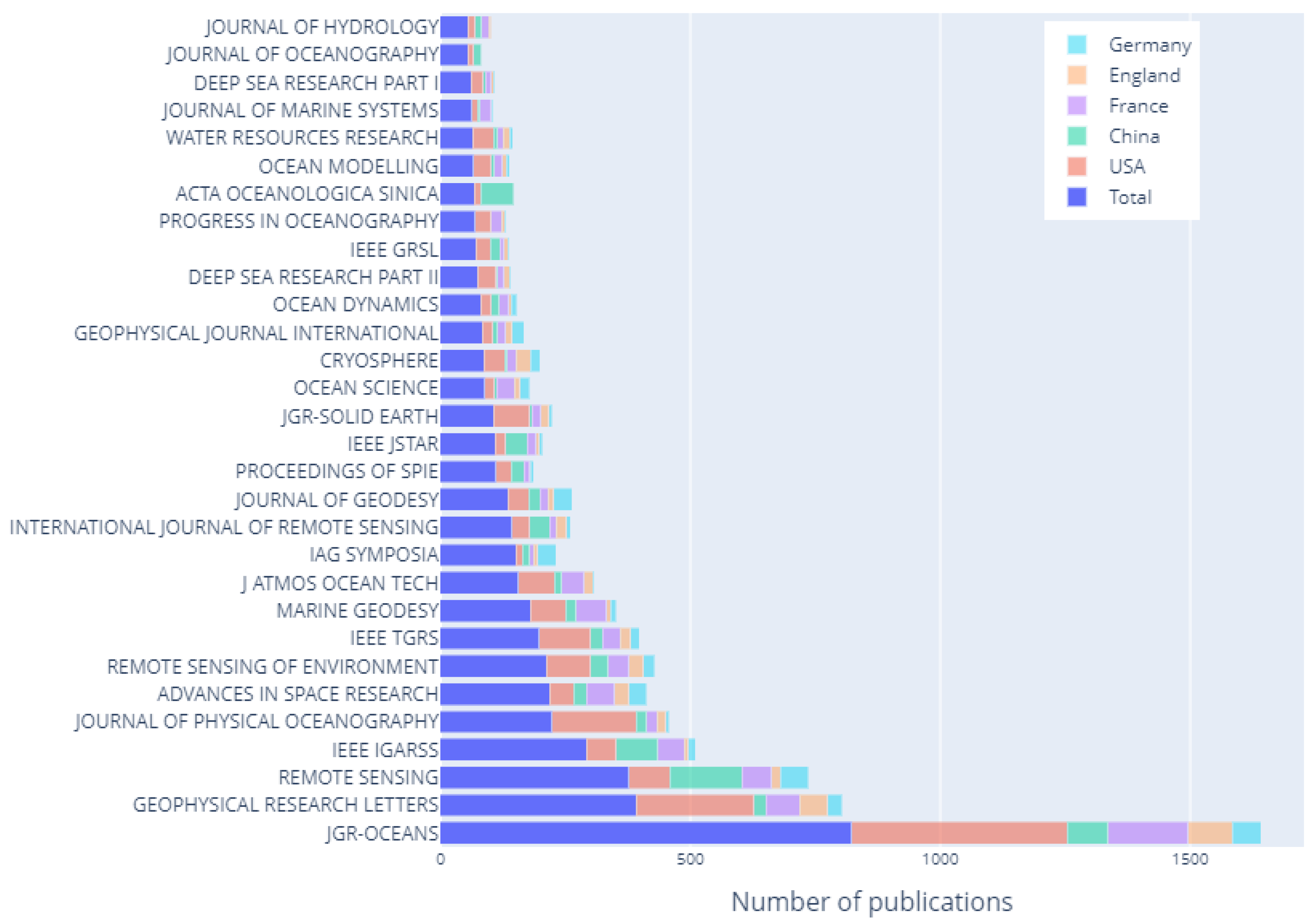
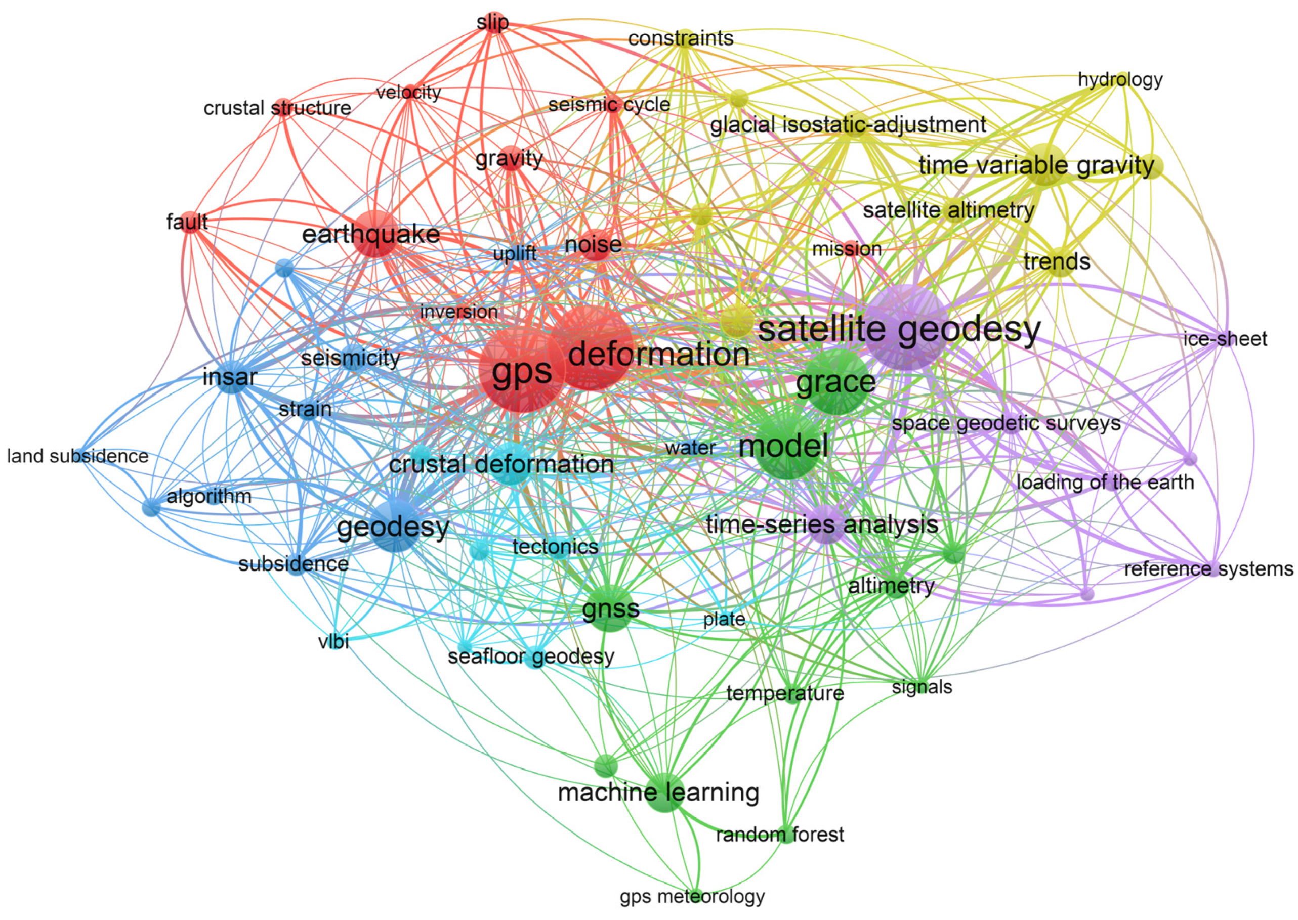
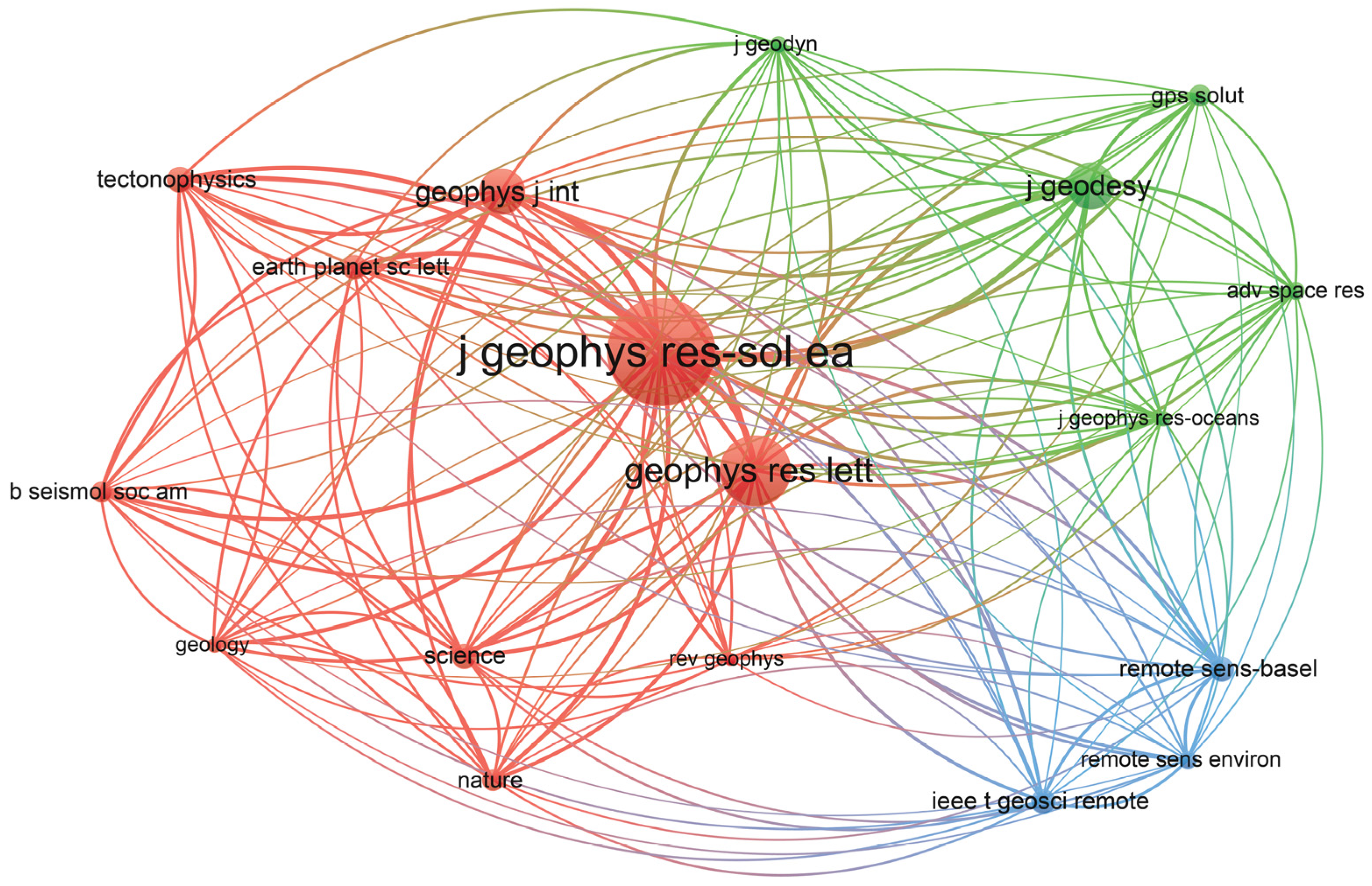
3.1. Some Statistics on the Papers Published in Geodetic Time Series during the Last Decade

The analysis of geodetic time series is crucial for many, if not all, areas of Environmental Geodesy. In the previous sections, we have underlined this need through the descriptions of several applications. Here, we focus on editorial analysis in terms of the number of papers published in the last decade, their theme, and their relationship using various keywords.
Figure 1 displays the number of articles published by various journals related to the topic “Geodetic Time Series and Applications for Earth Science and Environmental Monitoring” since 2010. We can observe that there have been about 11,000 items published. In addition, the figure shows the top 30 sources in terms of number of publications, as well as the relevant distribution for the top five nations. The Journal of Geophysical Research: Oceans, Geophysical Research Letters, and Remote Sensing rank as the top three journals in terms of the number of articles published, respectively. Note that US-based organizations and universities contribute to more than half of the publication volume for the JGR: Oceans and GRL journals, while Chinese-based organizations and universities contribute similarly to the studies published in Remote Sensing.
Figure 2 demonstrates the co-occurrence keywords retrieved from the selected journals displayed in Figure 1, which are then classified into five groups based on similarity. The highest ranked 10 keywords are Satellite Geodesy, Deformation, GPS, Model, GRACE, Time Variable Gravity, Time Series Analysis, Geodesy, Earthquake and GNSS.
Figure 3 displays the network of the scientific journals displayed in Figure 1 as a function of the co-citation within these selected journals. The analysis of Figure 3 shows that the top 10 co-cited journals are the Journal of Geophysical Research: Solid Earth, Geophysical Research Letters, Geophysical Journal International, Journal of Geodesy, Science, Remote Sensing, Earth and Planetary Science Letters, Tectonophysics, Advances in Space Research, and Journal of Nature.

3.2. Concluding Remarks on Contributions of the Special Issue of “Modelling Geodetic Time Series and Applications for Earth Science and Environmental Monitoring”

This Special Issue focuses on modelling the geodetic time series recorded by various instruments either onboard satellites or in fixed stations on the ground technologies (e.g., GNSS, GRACE, InSAR, and TLS) in order to monitor various geodynamics or seasonal phenomena and natural hazards. We emphasize the recent advances in the detection of small-amplitude transient signals, periodic signals, and long-term trends (e.g., seasonal signals, tectonic rate, etc.) that are contaminated by various types of noise (i.e., stochastic processes and correlations). Several papers have contributed to GNSS and its application to crustal deformation and geodynamics [63,64,65,66,67]; civil engineering [68,69]; stochastic noise modelling [70,71]; natural hazards such as landslides [36,37,72]; SLR estimation and coastal flooding [73,74,75]; hydrology, seasonal displacements, and drought monitoring using GNSS and/or GRACE/GRACE-FO [76,77,78]; and the study of ionospheric disturbances [79,80,81], together with research focused on the stability of the reference frame [82].
It is important to underline that these advanced methods explored in this Special Issue all have in common that they characterize and model the type of noises within the geodetic time series. It is necessary to carry out such modeling in order to accurately estimate geophysical signals to produce reliable results and better science. These techniques can be used to provide accurate results for assessing phenomena related to climate change (e.g., sea-level rise and regional droughts) and natural hazards (e.g., landslides and volcanic eruptions) which could jeopardize public safety. To some extent, this study intends to look at phenomena at both local and global scales combining various sources of data (e.g., satellites and fixed stations) in order to monitor and establish models of the changes in the earth’s natural phenomena (e.g., seasonal drought variations, climate anomalies, and sea-level rise acceleration).

Author Contributions

Conceptualization, X.H. and J.-P.M.; Data preparation, X.H.; Editorial Discussion, X.H., J.-P.M., G.K.; Original draft preparation J.-P.M.; Writing and editing, X.H., J.-P.M., G.K., R.F.; Review, all authors. All authors have read and agreed to the published version of the manuscript.

Funding

This work was sponsored by National Natural Science Foundation of China (42104023), 2022 Science and Technology Think Tank Young Talent Program (20220615ZZ07110308). This work was also supported by the project FCT/UID/GEO/50019/2019—IDL, funded by FCT.

Data Availability Statement

The data to produce Figure 1, Figure 2 and Figure 3 are available freely on Web of Science (www.webofscience.com).

Conflicts of Interest

The authors declare no conflict of interest.

References

  1. Collins, A. Gods of Eden: Egypt’s Lost Legacy and the Genesis of Civilization; Simon and Schuster: New York, NY, USA, 2002. [Google Scholar]
  2. Parker Pearson, M. Archaeology and legend: Investigating Stonehenge. Archaeol. Int. 2021, 24, 144–164. [Google Scholar] [CrossRef]
  3. Black, H.D. Early development of transit, the navy navigation satellite system. J. Guid. Control. Dyn. 1990, 13, 577–585. [Google Scholar] [CrossRef]
  4. Kolodziej, K.W.; Hjelm, J. Local Positioning Systems: LBS Applications and Services; CRC Press: Boca Raton, FL, USA, 2017. [Google Scholar]
  5. Karimi, H. An analysis of satellite visibility and single point positioning with GPS, GLONASS, Galileo, and BeiDou-2/3. Appl. Geomat. 2021, 13, 781–791. [Google Scholar] [CrossRef]
  6. Riecken, J.; Kurtenbach, E. Der Satellitenpositionierungsdienst der deutschen Landesvermessung–SAPOS®. Z. Geodäsie Geoinf. Landmanagement (ZfV) 2017, 142, 293–300. [Google Scholar]
  7. Jin, S.; van Dam, T.; Wdowinski, S. Observing and understanding the Earth system variations from space geodesy. J. Geodyn. 2013, 72, 1–10. [Google Scholar] [CrossRef] [Green Version]
  8. Bettinelli, P.; Avouac, J.P.; Flouzat, M.; Jouanne, F.; Bollinger, L.; Willis, P.; Chitrakar, G.R. Plate motion of India and interseismic strain in the Nepal Himalaya from GPS and DORIS measurements. J. Geod. 2006, 80, 567–589. [Google Scholar] [CrossRef]
  9. Montillet, J.P.; Williams, S.D.P.; Koulali, A.; McClusky, S.C. Estimation of offsets in GPS time-series and application to the detection of earthquake deformation in the far-field. Geophys. J. Int. 2015, 200, 1207–1221. [Google Scholar] [CrossRef] [Green Version]
  10. Tregoning, P.; Watson, C.; Ramillien, G.; McQueen, H.; Zhang, J. Detecting hydrologic deformation using GRACE and GPS. Geophys. Res. Lett. 2009, 36, 152. [Google Scholar] [CrossRef] [Green Version]
  11. Bos, M.S.; Penna, N.T.; Baker, T.F.; Clarke, P.J. Ocean tide loading displacements in western Europe: 2. GPS-observed anelastic dispersion in the asthenosphere. J. Geophys. Res. Solid Earth 2015, 120, 6540–6557. [Google Scholar] [CrossRef]
  12. Li, X.; Zus, F.; Lu, C.; Dick, G.; Ning, T.; Ge, M.; Wickert, J.; Schuh, H. Retrieving of atmospheric parameters from multi-GNSS in real time: Validation with water vapor radiometer and numerical weather model. J. Geophys. Res. Atmos. 2015, 120, 7189–7204. [Google Scholar] [CrossRef] [Green Version]
  13. Poutanen, M.; Rózsa, S. The geodesist’s handbook 2020. J. Geod. 2020, 94, 109. [Google Scholar] [CrossRef]
  14. Kouba, J. A Guide to Using International GNSS Service (IGS) Products; IGS: Ottawa, ON, Canada, 2009; Available online: https://kb.igs.org/hc/en-us/articles/201271873-A-Guide-to-Using-the-IGS-Products (accessed on 21 November 2022).
  15. Herring, T.A.; Melbourne, T.I.; Murray, M.H.; Floyd, M.A.; Szeliga, W.M.; King, R.W.; Phillips, D.A.; Puskas, C.M.; Santillan, M.; Wang, L. Plate Boundary Observatory and related networks: GPS data analysis methods and geodetic products. Rev. Geophys. 2016, 54, 759–808. [Google Scholar] [CrossRef]
  16. Langbein, J.; Svarc, J.L. Evaluation of temporally correlated noise in Global Navigation Satellite System time series: Geodetic monument performance. J. Geophys. Res. Solid Earth 2019, 124, 925–942. [Google Scholar] [CrossRef] [Green Version]
  17. He, X.; Bos, M.S.; Montillet, J.P.; Fernandes, R.; Melbourne, T.; Jiang, W.; Li, W. Spatial variations of stochastic noise properties in GPS time series. Remote Sens. 2021, 13, 4534. [Google Scholar] [CrossRef]
  18. Williams, S.D.; Bock, Y.; Fang, P.; Jamason, P.; Nikolaidis, R.M.; Prawirodirdjo, L.; Miller, M.; Johnson, D.J. Error analysis of continuous GPS position time series. J. Geophys. Res. Solid Earth 2004, 109, 443. [Google Scholar] [CrossRef] [Green Version]
  19. Beavan, J. Noise properties of continuous GPS data from concrete pillar geodetic monuments in New Zealand and comparison with data from US deep drilled braced monuments. J. Geophys. Res. Solid Earth 2005, 110, 80. [Google Scholar] [CrossRef]
  20. Michel, S.; Jolivet, R.; Lengliné, O.; Gualandi, A.; Larochelle, S.; Gardonio, B. Searching for Transient Slow Slips Along the San Andreas Fault Near Parkfield Using Independent Component Analysis. J. Geophys. Res. Solid Earth 2022, 127, e2021JB023201. [Google Scholar] [CrossRef]
  21. Bayik, C.; Abdikan, S.; Ozdemir, A.; Arıkan, M.; Balik Sanli, F.; Dogan, U. Investigation of the landslides in Beylikdüzü-Esenyurt Districts of Istanbul from InSAR and GNSS observations. Nat. Hazards 2021, 109, 1201–1220. [Google Scholar] [CrossRef]
  22. Crosta, G.B.; Agliardi, F.; Rivolta, C.; Alberti, S.; Dei Cas, L. Long-term evolution and early warning strategies for complex rockslides by real-time monitoring. Landslides 2017, 14, 1615–1632. [Google Scholar] [CrossRef]
  23. Carlà, T.; Tofani, V.; Lombardi, L.; Raspini, F.; Bianchini, S.; Bertolo, D.; Thuegaz, P.; Casagli, N. Combination of GNSS, satellite InSAR, and GBInSAR remote sensing monitoring to improve the understanding of a large landslide in high alpine environment. Geomorphology 2019, 335, 62–75. [Google Scholar] [CrossRef]
  24. Colesanti, C.; Wasowski, J. Investigating landslides with space-borne Synthetic Aperture Radar (SAR) interferometry. Eng. Geol. 2006, 88, 173–199. [Google Scholar] [CrossRef]
  25. Huang, M.H.; Fielding, E.J.; Liang, C.; Milillo, P.; Bekaert, D.; Dreger, D.; Salzer, J. Coseismic deformation and triggered landslides of the 2016 Mw 6.2 Amatrice earthquake in Italy. Geophys. Res. Lett. 2017, 44, 1266–1274. [Google Scholar] [CrossRef] [Green Version]
  26. Guo, H.; Yi, B.; Yao, Q.; Gao, P.; Li, H.; Sun, J.; Zhong, C. Identification of Landslides in Mountainous Area with the Combination of SBAS-InSAR and Yolo Model. Sensors 2022, 22, 6235. [Google Scholar] [CrossRef] [PubMed]
  27. Dong, D.; Fang, P.; Bock, Y.; Webb, F.; Prawirodirdjo, L.; Kedar, S.; Jamason, P. Spatiotemporal filtering using principal component analysis and Karhunen-Loeve expansion approaches for regional GPS network analysis. J. Geophys. Res. Solid Earth 2006, 111, 190. [Google Scholar] [CrossRef] [Green Version]
  28. Li, W.; Shen, Y.; Li, B. Weighted spatiotemporal filtering using principal component analysis for analyzing regional GNSS position time series. Acta Geod. Geophys. 2015, 50, 419–436. [Google Scholar] [CrossRef] [Green Version]
  29. Tiampo, K.F.; Mazzotti, S.; James, T.S. Analysis of GPS measurements in eastern Canada using principal component analysis. Pure Appl. Geophys. 2012, 16, 1483–1506. [Google Scholar] [CrossRef]
  30. He, X.; Montillet, J.P.; Fernandes, R.; Bos, M.; Yu, K.; Hua, X.; Jiang, W. Review of current GPS methodologies for producing accurate time series and their error sources. J. Geodyn. 2017, 106, 12–29. [Google Scholar] [CrossRef]
  31. Shen, Y.; Li, W.; Xu, G.; Li, B. Spatiotemporal filtering of regional GNSS network’s position time series with missing data using principal component analysis. J. Geod. 2014, 88, 1–12. [Google Scholar] [CrossRef]
  32. Yuan, L.G.; Ding, X.L.; Chen, W.; Kwok, S.; Chan, S.B.; Hung, P.S.; Chau, K.T. Characteristics of daily position time series from the Hong Kong GPS fiducial network. Chin. J. Geophys. 2008, 51, 976–990. [Google Scholar] [CrossRef]
  33. Davis, J.L.; Wernicke, B.P.; Tamisiea, M.E. On seasonal signals in geodetic time series. J. Geophys. Res. Solid Earth 2012, 117, 101. [Google Scholar] [CrossRef] [Green Version]
  34. Amiri-Simkooei, A.R. On the nature of GPS draconitic year periodic pattern in multivariate position time series. J. Geophys. Res. Solid Earth 2013, 118, 2500–2511. [Google Scholar] [CrossRef]
  35. Barbarella, M.; Fiani, M. Monitoring of large landslides by Terrestrial Laser Scanning techniques: Field data collection and processing. Eur. J. Remote Sens. 2013, 46, 126–151. [Google Scholar] [CrossRef]
  36. Zhu, X.; Zhang, F.; Deng, M.; Liu, J.; He, Z.; Zhang, W.; Gu, X. A Hybrid Machine Learning Model Coupling Double Exponential Smoothing and ELM to Predict Multi-Factor Landslide Displacement. Remote Sens. 2022, 14, 3384. [Google Scholar] [CrossRef]
  37. Huang, D.; He, J.; Song, Y.; Guo, Z.; Huang, X.; Guo, Y. Displacement Prediction of the Muyubao Landslide Based on a GPS Time-Series Analysis and Temporal Convolutional Network Model. Remote Sens. 2022, 14, 2656. [Google Scholar] [CrossRef]
  38. Kermarrec, G.; Skytt, V.; Dokken, T. Surface approximation of coastal regions: LR B-spline for detection of deformation pattern. ISPRS Ann. Photogramm. Remote Sens. Spat. Inf. Sci. 2022, V-2-2022, 119–126. [Google Scholar] [CrossRef]
  39. Church, J.A.; White, N.J. Sea-level rise from the late 19th to the early 21st century. Surv. Geophys. 2011, 32, 585–602. [Google Scholar] [CrossRef] [Green Version]
  40. Oppenheimer, M.; Glavovic, B.; Hinkel, J.; van de Wal, R.; Magnan, A.K.; Abd-Elgawad, A.; Sebesvari, Z. Sea Level Rise and Implications for Low Lying Islands, Coasts and Communities. Chapter 4, IPPCC report. 2019. Available online: https://www.ipcc.ch/srocc/chapter/chapter-4-sea-level-rise-and-implications-for-low-lying-islands-coasts-and-communities/ (accessed on 21 November 2022).
  41. Walkden, P. Complexities of coastal resilience. Nat. Geosci. 2022, 15. [Google Scholar] [CrossRef]
  42. Hannah, J.; Bell, R.G. Regional sea level trends in New Zealand. J. Geophys. Res. Ocean. 2012, 117, 36. [Google Scholar] [CrossRef]
  43. Raj, N.; Gharineiat, Z.; Ahmed, A.A.M.; Stepanyants, Y. Assessment and Prediction of Sea Level Trend in the South Pacific Region. Remote Sens. 2022, 14, 986. [Google Scholar] [CrossRef]
  44. Panet, I.; Mikhailov, V.; Diament, M.; Pollitz, F.; King, G.; De Viron, O.; Holschneider, M.; Biancale, R.; Lemoine, J.M. Coseismic and post-seismic signatures of the Sumatra 2004 December and 2005 March earthquakes in GRACE satellite gravity. Geophys. J. Int. 2007, 171, 177–190. [Google Scholar] [CrossRef] [Green Version]
  45. Denys, P.H.; Beavan, R.J.; Hannah, J.; Pearson, C.F.; Palmer, N.; Denham, M.; Hreinsdottir, S. Sea level rise in New Zealand: The effect of vertical land motion on century-long tide gauge records in a tectonically active region. J. Geophys. Res. Solid Earth 2020, 125, e2019JB018055. [Google Scholar] [CrossRef]
  46. Montillet, J.P.; Melbourne, T.I.; Szeliga, W.M. GPS vertical land motion corrections to sea-level rise estimates in the Pacific Northwest. J. Geophys. Res. Ocean. 2018, 123, 1196–1212. [Google Scholar] [CrossRef]
  47. Agnew, D.C. The time-domain behavior of power-law noises. Geophys. Res. Lett. 1992, 19, 333–336. [Google Scholar] [CrossRef]
  48. Hughes, C.W.; Williams, S.D. The color of sea level: Importance of spatial variations in spectral shape for assessing the significance of trends. J. Geophys. Res. Ocean. 2010, 115, 59. [Google Scholar] [CrossRef] [Green Version]
  49. Armitage, T.W.; Bacon, S.; Ridout, A.L.; Thomas, S.F.; Aksenov, Y.; Wingham, D.J. Arctic sea surface height variability and change from satellite radar altimetry and GRACE, 2003–2014. J. Geophys. Res. Ocean. 2016, 121, 4303–4322. [Google Scholar] [CrossRef] [Green Version]
  50. Liibusk, A.; Kall, T.; Rikka, S.; Uiboupin, R.; Suursaar, Ü.; Tseng, K.H. Validation of copernicus sea level altimetry products in the baltic sea and estonian lakes. Remote Sens. 2020, 12, 4062. [Google Scholar] [CrossRef]
  51. Chen, J.; Cazenave, A.; Dahle, C.; Llovel, W.; Panet, I.; Pfeffer, J.; Moreira, L. Applications and challenges of GRACE and GRACE follow-on satellite gravimetry. Surv. Geophys. 2022, 43, 305–345. [Google Scholar] [CrossRef]
  52. Frappart, F.; Ramillien, G. Monitoring groundwater storage changes using the Gravity Recovery and Climate Experiment (GRACE) satellite mission: A review. Remote Sens. 2018, 10, 829. [Google Scholar] [CrossRef] [Green Version]
  53. García-García, D.; Ummenhofer, C.C.; Zlotnicki, V. Australian water mass variations from GRACE data linked to Indo-Pacific climate variability. Remote Sens. Environ. 2011, 115, 2175–2183. [Google Scholar] [CrossRef] [Green Version]
  54. Longuevergne, L.; Scanlon, B.R.; Wilson, C.R. GRACE Hydrological estimates for small basins: Evaluating processing approaches on the High Plains Aquifer, USA. Water Resour. Res. 2010, 46, 215. [Google Scholar] [CrossRef]
  55. Strassberg, G.; Scanlon, B.R.; Rodell, M. Comparison of seasonal terrestrial water storage variations from GRACE with groundwater-level measurements from the High Plains Aquifer (USA). Geophys. Res. Lett. 2007, 34, 141. [Google Scholar] [CrossRef]
  56. Allgeyer, S.; Tregoning, P.; McQueen, H.; McClusky, S.C.; Potter, E.K.; Pfeffer, J.; McGirr, R.; Purcell, A.P.; Herring, T.A.; Montillet, J.P. ANU GRACE Data Analysis: Orbit Modeling, Regularization and Inter-satellite Range Acceleration Observations. J. Geophys. Res. Solid Earth 2022, 127, e2021JB022489. [Google Scholar] [CrossRef]
  57. Carlson, G.; Werth, S.; Shirzaei, M. Joint Inversion of GNSS and GRACE for Terrestrial Water Storage Change in California. J. Geophys. Res. Solid Earth 2022, 127, e2021JB023135. [Google Scholar] [CrossRef] [PubMed]
  58. Wang, H.; Xiang, L.; Steffen, H.; Wu, P.; Jiang, L.; Shen, Q.; Li, Z.; Hayashi, M. GRACE-based estimates of groundwater variations over North America from 2002 to 2017. Geod. Geodyn. 2022, 13, 11–23. [Google Scholar] [CrossRef]
  59. Klos, A.; Bogusz, J.; Figurski, M.; Kosek, W. On the handling of outliers in the GNSS time series by means of the noise and probability analysis. In IAG 150 Years; Springer: Cham, Germany, 2015; pp. 657–664. [Google Scholar]
  60. Williams, S.D.P.; Penna, N.T. Non-tidal ocean loading effects on geodetic GPS heights. Geophys. Res. Lett. 2011, 38, 76. [Google Scholar] [CrossRef] [Green Version]
  61. Hofmann-Wellenhof, B.; Lichtenegger, H.; Collins, J. Global Positioning System: Theory and Practice; Springer Science & Business Media: Berlin, Germany, 2012. [Google Scholar]
  62. Poli, P.; Pailleux, J.; Ducrocq, V.; Moll, P.; Rabier, F.; Mauprivez, M.; Dufour, S.; Grondin, M.; Carvalho, F.; Issler, J.L.; et al. Weather report: Meteorological applications of GNSS from space and on the ground. InsideGNSS 2008, 3, 30–39. [Google Scholar]
  63. Xi, R.; Liang, Y.; Chen, Q.; Jiang, W.; Chen, Y.; Liu, S. Analysis of Annual Deformation Characteristics of Xilongchi Dam Using Historical GPS Observations. Remote Sens. 2022, 14, 4018. [Google Scholar] [CrossRef]
  64. Wang, H.; Ren, Y.; Wang, A.; Wang, J.; Cheng, Y.; Fang, S.; Yang, Q. Two-Decade GNSS Observation Processing and Analysis with the New IGS Repro3 Criteria: Implications for the Refinement of Velocity Field and Deformation Field in Continental China. Remote Sens. 2022, 14, 3719. [Google Scholar] [CrossRef]
  65. Hu, S.; Chen, K.; Zhu, H.; Xue, C.; Wang, T.; Yang, Z.; Zhao, Q. A Comprehensive Analysis of Environmental Loading Effects on Vertical GPS Time Series in Yunnan, Southwest China. Remote Sens. 2022, 14, 2741. [Google Scholar] [CrossRef]
  66. Li, W.; Li, F.; Shum, C.K.; Shu, C.; Ming, F.; Zhang, S.; Zhang, Q.; Chen, W. Assessment of Contemporary Antarctic GIA Models Using High-Precision GPS Time Series. Remote Sens. 2022, 14, 1070. [Google Scholar] [CrossRef]
  67. Xiang, Y.; Wang, H.; Chen, Y.; Xing, Y. GNSS Imaging of Strain Rate Changes and Vertical Crustal Motions over the Tibetan Plateau. Remote Sens. 2021, 13, 4937. [Google Scholar] [CrossRef]
  68. Mao, W.; Liu, G.; Wang, X.; Xie, Y.; He, X.; Zhang, B.; Xiang, W.; Wu, S.; Zhang, R.; Fu, Y.; et al. Using Range Split-Spectrum Interferometry to Reduce Phase Unwrapping Errors for InSAR-Derived DEM in Large Gradient Region. Remote Sens. 2022, 14, 2607. [Google Scholar] [CrossRef]
  69. Zhou, R.; Hu, Z.; Zhao, Q.; Cai, H.; Liu, X.; Liu, C.; Wang, G.; Kan, H.; Chen, L. Consistency Analysis of the GNSS Antenna Phase Center Correction Models. Remote Sens. 2022, 14, 540. [Google Scholar] [CrossRef]
  70. Xu, C.; Yao, X.; He, X. Noise Analysis and Combination of Hydrology Loading-Induced Displacements. Remote Sens. 2022, 14, 2840. [Google Scholar] [CrossRef]
  71. Li, W.; Li, Z.; Jiang, W.; Chen, Q.; Zhu, G.; Wang, J. A New Spatial Filtering Algorithm for Noisy and Missing GNSS Position Time Series Using Weighted Expectation Maximization Principal Component Analysis: A Case Study for Regional GNSS Network in Xinjiang Province. Remote Sens. 2022, 14, 1295. [Google Scholar] [CrossRef]
  72. Peng, Y.; Dong, D.; Chen, W.; Zhang, C. Stable Regional Reference Frame for Reclaimed Land Subsidence Study in East China. Remote Sens. 2022, 14, 3984. [Google Scholar] [CrossRef]
  73. He, X.; Montillet, J.P.; Fernandes, R.; Melbourne, T.I.; Jiang, W.; Huang, Z. Sea Level Rise Estimation on the Pacific Coast from Southern California to Vancouver Island. Remote Sens. 2022, 14, 4339. [Google Scholar] [CrossRef]
  74. Gruber, T.; Ågren, J.; Angermann, D.; Ellmann, A.; Engfeldt, A.; Gisinger, C.; Jaworski, L.; Kur, T.; Marila, S.; Nastula, J.; et al. Geodetic SAR for Height System Unification and Sea Level Research—Results in the Baltic Sea Test Network. Remote Sens. 2022, 14, 3250. [Google Scholar] [CrossRef]
  75. Szelachowska, M.; Godah, W.; Krynski, J. Contribution of GRACE Satellite Mission to the Determination of Orthometric/Normal Heights Corrected for Their Dynamics—A Case Study of Poland. Remote Sens. 2022, 14, 4271. [Google Scholar] [CrossRef]
  76. Cui, L.; Yin, M.; Huang, Z.; Yao, C.; Wang, X.; Lin, X. The drought events over the Amazon River basin from 2003 to 2020 detected by GRACE/GRACE-FO and Swarm satellites. Remote Sens. 2022, 14, 2887. [Google Scholar] [CrossRef]
  77. Liu, B.; Yu, W.; Dai, W.; Xing, X.; Kuang, C. Estimation of Terrestrial Water Storage Variations in Sichuan-Yunnan Region from GPS Observations Using Independent Component Analysis. Remote Sens. 2022, 14, 282. [Google Scholar] [CrossRef]
  78. Liu, H.; Zhou, Y.; Ray, J.; Luo, J. Excitations of Seasonal Polar Motions Derived from Satellite Gravimetry and General Circulation Models: Comparisons of Harmonic and Inharmonic Analyses. Remote Sens. 2022, 14, 3567. [Google Scholar] [CrossRef]
  79. Xia, G.; Liu, M.; Zhang, F.; Zhou, C. CAiTST: Conv-Attentional Image Time Sequence Transformer for Ionospheric TEC Maps Forecast. Remote Sens. 2022, 14, 4223. [Google Scholar] [CrossRef]
  80. Tang, J.; Li, Y.; Yang, D.; Ding, M. An Approach for Predicting Global Ionospheric TEC Using Machine Learning. Remote Sens. 2022, 14, 1585. [Google Scholar] [CrossRef]
  81. Kong, J.; Shan, L.; Yan, X.; Wang, Y. Analysis of Ionospheric Disturbance Response to the Heavy Rain Event. Remote Sens. 2022, 14, 510. [Google Scholar] [CrossRef]
  82. Yang, R.; Deng, C.; Yu, K.; Li, Z.; Pan, L. A New Way for Cartesian Coordinate Transformation and Its Precision Evaluation. Remote Sens. 2022, 14, 864. [Google Scholar] [CrossRef]
Figure 1. Histogram of the number of papers published within several journals using keywords (i.e., Geodetic Time Series, GNSS time series, Crustal Deformation Geodesy, Environmental Monitoring, InSAR Geodesy, Machine Learning Geodesy, Sea Level Rise Geodesy, Tectonic Activity Geodesy and Terrestrial Laser Scanners Geodesy). The source of the statistics is web of science.
Remotesensing 14 06164 g001
Figure 2. The network of the co-occurrence keywords retrieved from the selected journals displayed in Figure 1. Note that we set the limit of the connections threshold in order to present only the 14 highest ranked words.
Remotesensing 14 06164 g002
Figure 3. Network of the scientific journals displayed in Figure 1 as a function of the co-citation within these selected journals. We set the limit of the connections threshold in order to present only the 18 highest ranked results.
Remotesensing 14 06164 g003
Publisher’s Note: MDPI stays neutral with regard to jurisdictional claims in published maps and institutional affiliations.

