Article

Trend Analysis and Driving Factors of Vegetation Dynamics in Northern China from 1982 to 2015

1
Key Laboratory of Water Cycle and Related Land Surface Processes, Institute of Geographic Sciences and Natural Resources Research, Chinese Academy of Sciences, Beijing 100101, China
2
College of Resources and Environment, University of Chinese Academy of Sciences, Beijing 100049, China
3
Department of Civil, Environmental and Geomatics Engineering, Florida Atlantic University, Boca Raton, FL 33431, USA
*
Author to whom correspondence should be addressed.
Remote Sens. 2022, 14(23), 6163; https://doi.org/10.3390/rs14236163
Submission received: 7 October 2022 / Revised: 20 November 2022 / Accepted: 1 December 2022 / Published: 5 December 2022

Abstract

:
Under the background of global warming, understanding the dynamic of vegetation plays a key role in revealing the structure and function of an ecosystem. Assessing the impact of climate change and human activities on vegetation dynamics is crucial for policy formulation and ecological protection. Based on the Global Inventory Monitoring and Modeling System (GIMMS) third generation of Normalized Difference Vegetation Index (NDVI3g), meteorological data and land cover data, this study analyzed the linear and nonlinear trends of vegetation in northern China from 1982 to 2015, and quantified the relative impact of climate change and human activities on vegetation change. The results showed that more than 53% of the vegetation had changed significantly, and 36.64% of the vegetation had a reverse trend. There were potential risks of vegetation degradation in the southwestern, northwestern and northeastern parts of the study’s area. The linear analysis method cannot disclose the reversal of the vegetation growth trend, which will underestimate or overestimate the risk of vegetation degradation or restoration. Climate change and human activities promoted 76.54% of the vegetation growth in the study area, with an average contribution rate of 51.22% and 48.78%, respectively, while the average contribution rate to the vegetation degradation area was 47.43% and 52.57%, respectively. Vegetation restoration of grassland and woodland was mainly affected by climate change, and human activities dominated their degradation, while cropland vegetation was opposite. The contribution rate of human activities to vegetation change in the southeastern and eastern parts of the study area was generally higher than that of climate change, but it was the opposite in the high altitude area, with obvious spatial heterogeneity. These results are helpful to understand the dynamic mechanism of vegetation in northern China, and provide a scientific basis for vegetation restoration and protection of regional ecosystems.

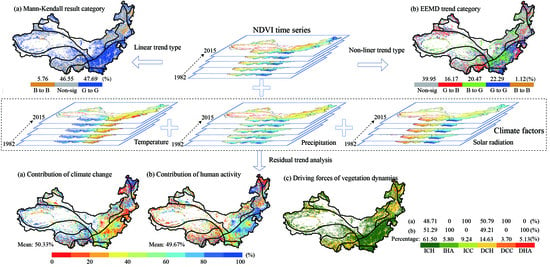
Graphical Abstract

1. Introduction

The dynamic change of vegetation can affect global carbon, the water cycle and energy flow [1], and is considered an indicator of ecosystems’ health [2,3]. Vegetation plays an indispensable role in maintaining regional ecological balance, especially in reducing soil erosion [4]. Therefore, monitoring vegetation dynamics and analyzing their drivers are very important for studying global climate change and ecological environment protection and restoration [5,6].
The rapid development of satellite remote sensing provides a series of continuous spatiotemporal observation data for scientific research [7]. Remote sensing data have become an important source in the field of ecological environment monitoring because of their advantages such as large space coverage, easy access, rich information and continuous time scale [8,9]. The normalized difference vegetation index (NDVI) calculated from red and near-infrared reflectances is considered an effective indicator to evaluate vegetation growth state [7], and has good correlation with leaf area, photosynthetically active radiation absorption, and vegetation productivity [10]; therefore, it is often used to study vegetation dynamics and monitor the ecological environment [5,11]. The increase (greening) or decrease (browning) of NDVI can directly reflect the enhancing or weakening of vegetation activity [12]. Therefore, correctly describing vegetation dynamics is the key to understanding the impact of climate change on terrestrial ecosystems [12].
Northern China includes several typical areas, such as the Loess Plateau, Xinjiang, Inner Mongolia, Qilian Mountains and Qinghai Plateau, which are the key areas for water and soil conservation, vegetation protection and restoration [13]. In the past few decades, in order to protect and improve the regional ecological environment, the Chinese government has launched a series of large-scale ecological protection and restoration projects, such as the “Grain for Green Program” [13], “Natural Forest Conservation Program” [14], “Three North Shelterbelt Development Program” [15], and the “Beijing-Tianjin Sand Source Control Program” [16]. The implementation of ecological projects can significantly improve the vegetation coverage and ecological environment [17,18]. The driving factors of vegetation dynamics can be divided into climate factors and human activities. An accurate description of the vegetation dynamic process is helpful to accurately evaluate the relative contribution of climate change and human activities to vegetation dynamics, and to divide the different driving forces of vegetation dynamics, which is of great significance for ecosystem protection and policy formulation [7].
At present, simple linear models are used by many researchers to describe the process of vegetation change, assuming that the process of vegetation change is monotonic with a constant trend [12]. However, the growth process of vegetation is unstable and nonlinear, which changes with time [19]. Therefore, the linear trend analysis method may ignore the potential greening or browning trend of vegetation during the study period [10,12]. A nonlinear analysis method is considered effective for analyzing vegetation dynamics [7], mainly including piecewise linear regression model [20], breaks for additive seasonal and trend (BFAST) [21], detecting breakpoints and estimating segments in trend (DBEST) [22], etc. The above methods are very sensitive to short-term fluctuations and abrupt changes, which weakens their ability to detect trend shifts and turning points in long time series [12]. Wavelet analysis needs to select basic functions, which also limits its application in vegetation dynamics [23]. The ensemble empirical mode decomposition (EEMD) [24] is usually used to study the time series trend of variables in signal and image processing [25], climate diagnosis [26], hydrology [27] and other fields. EEMD does not need to determine the basic function, and has good adaptability [12]. At the same time, EEMD decomposition can reveal more potential information of nonlinear and non-stationary time series of vegetation [6], which has been applied in the remote sensing field [10,23,28,29].
The vegetation types in northern China are complex and diverse, with most of them being located in semi-arid and arid areas, and the natural ecological environment is very complex and fragile [30]. Therefore, analyzing the nonlinear change characteristics of vegetation will help us to better understand the dynamics of vegetation and its relationship with driving factors [7]. At present, most of the relevant studies focus on typical ecological study areas [7,31], while few studies focus on the whole of northern China, lacking a comprehensive analysis of the spatial distribution of vegetation greening, browning and trend reversal. Therefore, in order to deeply understand the vegetation dynamics and its driving mechanism in northern China, the purpose of this study is to (a) analyze the spatial pattern of linear and nonlinear changes in vegetation, (b) analyze the nonlinear characteristics of vegetation in different land cover and climatic zones, (c) assess the response of vegetation with different trends to climate change, and (d) quantify the relative contributions of climate change and human activities to vegetation change.

2. Materials and Methods

2.1. Study Area

The study area is located in northern China, which lies between 73°37′–125°57′E and 31°41′–53°18′N, with a total area of about 4,497,784 km2. This study area covers three steps of China’s terrain, with obvious differences in altitude, ranging from −156 to 7347 m. The altitude in the west and southwest of the study area is relatively high, while that in the east is relatively low. The monthly average temperature is about 4.37 °C, and the monthly average precipitation is about 23.48 mm. According to the precipitation, it can be divided into arid, sub-arid, sub-humid and humid areas, of which arid and semi-arid areas are the main types of the study area. According to the climatic zone, it is divided into subtropical, warm temperate, middle temperate, cold temperate, and plateau climate zones. The study area is mainly covered by warm temperate, middle temperate and plateau climate zones [32] (Figure 1). Therefore, there are regional differences in hydrothermal environment in the study area (Table 1), forming a unique terrestrial ecosystem. Grassland is the main land cover type in the study area (Figure 1c).

2.2. Data and Preprocessing

2.2.1. GIMMS NDVI3g

GIMMS NDVI3g, with 8 km spatial resolution and 15-day temporal resolution, is composed of upper and lower scene data every month, and the time span ranges from July 1981 to December 2015. Although the spatial resolution of GIMMS NDVI3g is relatively low, its time series is the longest and can reflect the change trend of NDVI more comprehensively than other products [33]. Therefore, GIMMS NDVI3g has been widely used for global or regional scale vegetation change monitoring [12]. High quality NDVI time series data are of great significance for regional and global ecological and environmental application research. In this study, spatial–temporal Savitzky–Golay (STSG) filter proposed by Cao [34] was used to smooth NDVI data, so as to further improve the quality of GIMMS NDVI3g. Finally, the filtered GIMMS NDVI3g was aggregated into monthly NDVI data by Maximum Value Composite (MVC) [35]. Combined with previous studies, the vegetation growth season was defined as April to October [36], and the NDVI in the growth season (GSN) was obtained by calculating the average value from April to October.

2.2.2. Meteorological Datasets

The meteorological data included precipitation and temperature, which came from the daily value dataset of surface climate data (V3.0) provided by China Meteorological Data Service Center (http://data.cma.cn/ (accessed on 21 May 2018)), including 829 meteorological stations, with a time range from 1981 to 2015. The monthly raster data with the same spatial resolution as GIMMS NDVI3g were obtained by interpolating the meteorological station data with digital elevation model (DEM) data and ANUSPLIN 4.2 software [37]. The DEM data were collected from the NASA Shuttle Radar Topographic Mission [23].
The monthly radiation raster data were downloaded from ERA5 of the European Centre for Medium-Range Weather Forecasts (ECMWF) (https://www.ecmwf.int/ (accessed on 12 July 2019)), which was the fifth generation ECMWF atmospheric reanalysis of the global climate covering the period from January 1950 to present, with a spatial resolution of 0.25 degrees. Similarly, we used ANUSPLIN 4.2 software and DEM data to interpolate the solar radiation data to match the spatial resolution of GIMMS NDVI3g.
Finally, we calculated the mean temperature (GS-Tem), cumulative precipitation (GS-Pre) and mean solar radiation (GS-SR) in the growing season of vegetation.

2.2.3. Other Geospatial Ancillary Data

The land cover data and climate zone data were derived from Data Center for Resources and Environmental Sciences, Chinese Academy of Sciences (RESDC, http://www.resdc.cn (accessed on 1 August 2019)). The land cover data contain seven periods of land cover data, with a spatial resolution of 1 km and a time span from 1980 to 2015. The first-class classification accuracy exceeds 94.3% [38], and has been widely used in relevant research on a regional scale [30,39,40]. The land cover data were resampled to the same spatial resolution as GIMMS NDVI3g using the nearest neighbor resampling method. In order to reduce the impact of land cover change and classification errors, we only selected the grids with unchanged land cover types from 1980 to 2015. The vegetation cover types included cropland, woodland and grassland, which accounted for 18.43%, 16.02% and 65.55% of the total area (referring to the total area of cropland, woodland and grassland).

2.3. Method

2.3.1. Sen Median Trend Analysis and Mann–Kendall Test

Sen median trend analysis and the Mann–Kendall test are widely used in trend analysis of meteorological, hydrological and remote sensing time series [33,41]. Sen median trend analysis can avoid the interference of outliers well, which is more suitable for studying vegetation change trend [42]. The calculation formula can refer to previous studies [42].
The Mann–Kendall test was used to judge the significance of time series trend. The formula of the Mann–Kendall test can refer to previous studies [30]. In the study, α was set to 0.05, and the NDVI trend was divided into three types: monotonic browning (B to B) (ρ < 0, |Z| > 1.96, p < 0.05), monotonic greening (G to G) (ρ > 0, |Z| > 1.96, p < 0.05) and non-significant change (Non-sig) (|Z| ≤ 1.96, p > 0.05).

2.3.2. Ensemble Empirical Mode Decomposition (EEMD) Method

Wu [24], aiming at overcoming the shortcomings of empirical mode decomposition (EMD), proposed ensemble empirical mode decomposition (EEMD) based on EMD. EEMD uses Gaussian white noise to assist the original data. After the amplitude of white noise meets certain conditions, after several calculations, the set average is enough to make the white noise cancel each other, and its value will not have a significant impact on the decomposition results. EEMD method has strong adaptability and avoids human experience interference [12]. Therefore, we used EEMD to study the nonlinear change characteristics of vegetation, and obtained the trend component that could reflect the long-term trend of the original time series data. The decomposition steps of EEDM can refer to previous studies [12,29].
Considering the calculation time and robustness of EEMD [12], the number of Gaussian white noise added in this study was set to 100, and the noise amplitude was 0.2 standard deviation of the original time series data.
In order to compare with the linear trend, we used the average changing rate of instantaneous trend as the average EEMD trend of NDVI time series during the study period [12,28], which was the EEMD trend of the last year divided by the time interval.
T rend e e m d   =   R n ( t e n d ) R n ( t 0 ) t e n d t 0
where t0 and tend represent the time at the beginning and end of the study, respectively.
Similarly, we used the method of Pan et al. [12] to test the significance of EEMD trend. According to the significance test and extreme points, the EEMD trend of NDVI was divided into five types:
(1)
Non-significant (Non-sig): the trends were not significant at any year (p > 0.05).
(2)
Greening to greening (G to G): the trends were monotonic increasing and were statistically significant for at least one year (p < 0.05).
(3)
Browning to browning (B to B): the trends were monotonic decreasing and were statistically significant for at least one year (p < 0.05).
(4)
Greening to browning (G to B): the trends contained one local maximum, which changed from increasing trend to decreasing trend, and were statistically significant for at least one year (p < 0.05).
(5)
Browning to greening (B to G): the trends contained one local minimum, which changed from decreasing trend to increasing trend, and were statistically significant for at least one year (p < 0.05).
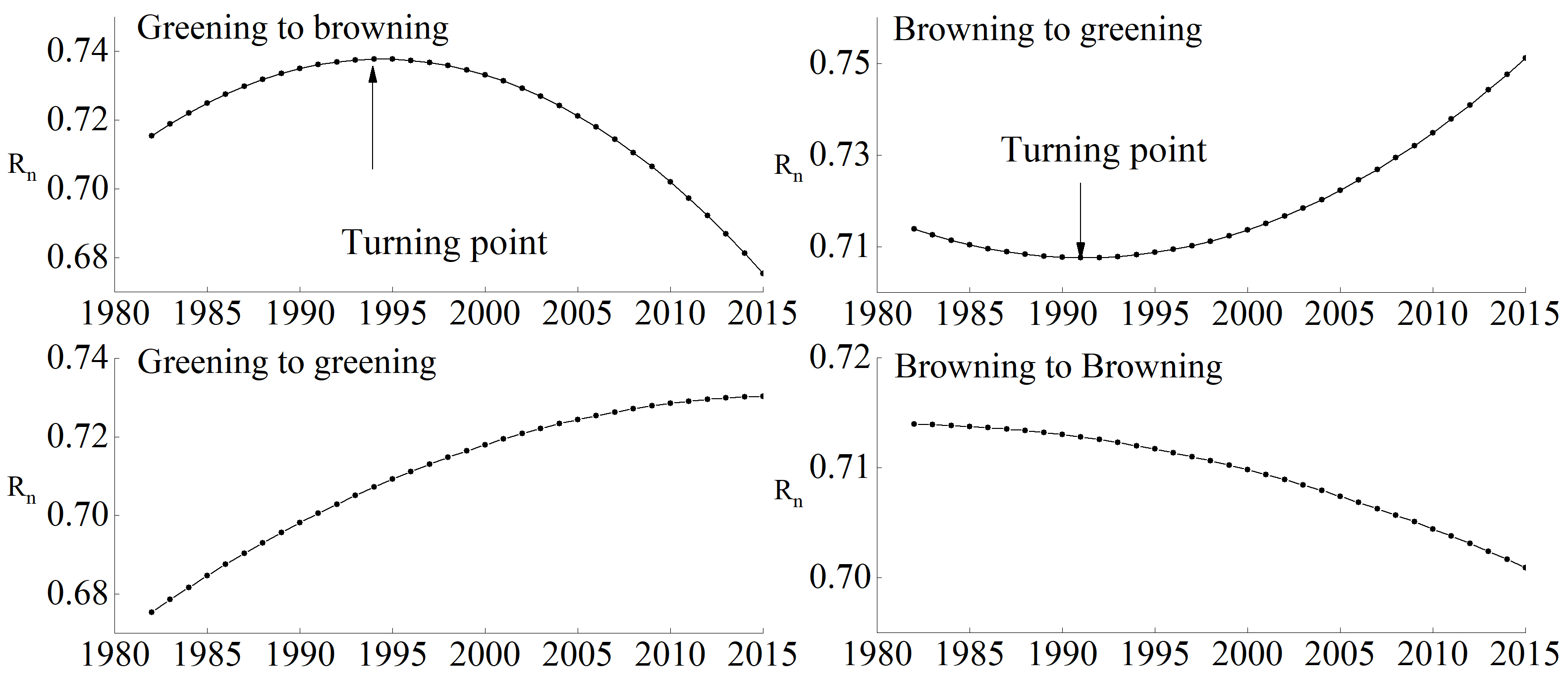
Four pixels in the study area were randomly selected to show different types of NDVI EEMD trends (Figure 2). The trend component Rn represents the long-term change trend of NDVI time series. For trends with one extreme value, the location of the extreme value is identified as the turning point (TP). Monotonic greening and browning were collectively referred to as monotonic trend. Greening to browning and browning to greening were collectively referred to as reversal trend.

2.3.3. Partial Correlation Analysis

For multivariate correlation analysis, Pearson correlation analysis cannot exclude the impact of mutual correlation between other climate factors on NDVI. Therefore, a partial correlation coefficient (PCC) was used to calculate the impact of a single climate factor on vegetation growth by treating other climate factors as control variables. For three climate factors, PCC is as follows:
R 12 , 34   =   R 12 , 3 R 14 , 3 × R 24 , 3 ( 1 R 14 , 3 2 ) × ( 1 R 24 , 3 2 )
R 12 , 3   =   R 12 R 13 × R 23 ( 1 R 13 2 ) × ( 1 R 23 2 )
where R 12 , 34 refers to the PCC of variables 1 and 2, and variables 3 and 4 are the control variables;   R 12 , 3 refers to the PCC of variables 1 and 2, and variable 3 is the control variable;   R 12 refers to the correlation coefficient of variables 1 and 2. Similarly, other variables have similar meanings. Variable 1 refers to NDVI, and variables 2, 3, and 4 represent three climatic factors, respectively. The PCC between NDVI and each climatic factor was calculated. The t-test was used to estimate the significance of the calculated PCC in the case of p < 0.05.

2.3.4. Residual Trend (RESTREND) Analysis

The driving factors of vegetation dynamics include climate and non-climate factors, with non-climate factors usually being considered as human activities [43]. The residual trend analysis method is usually used to distinguish the impact of human activities and climate change on vegetation change [39,44]. Firstly, multiple linear regression is used to simulate the predicted value of NDVI under the influence of climate change (NDVIc). Then, calculate the NDVI value affected by human activities (NDVIh), which is the difference between the actual NDVI and NDVIc. The positive or negative slopes of NDVIc and NDVIh indicate whether climate change and human activities promote vegetation growth, respectively.
NDVI c   =   p 0   +   p 1 T e m   +   p 2 P r e   +   p 3 S R   +   ε
NDVI h   =   NDVI     NDVI c
where Tem, Pre, and SR are the temperature, precipitation, and solar radiation, respectively; p 0   p 1 , p 2 and p 3 are the fitting coefficients; and ε is the residual error term.
According to previous studies [28,41,44], climate change and human activities can be divided into six scenarios according to the positive and negative relationship among NDVI, NDVIc and NDVIh slopes, as shown in Table 2.
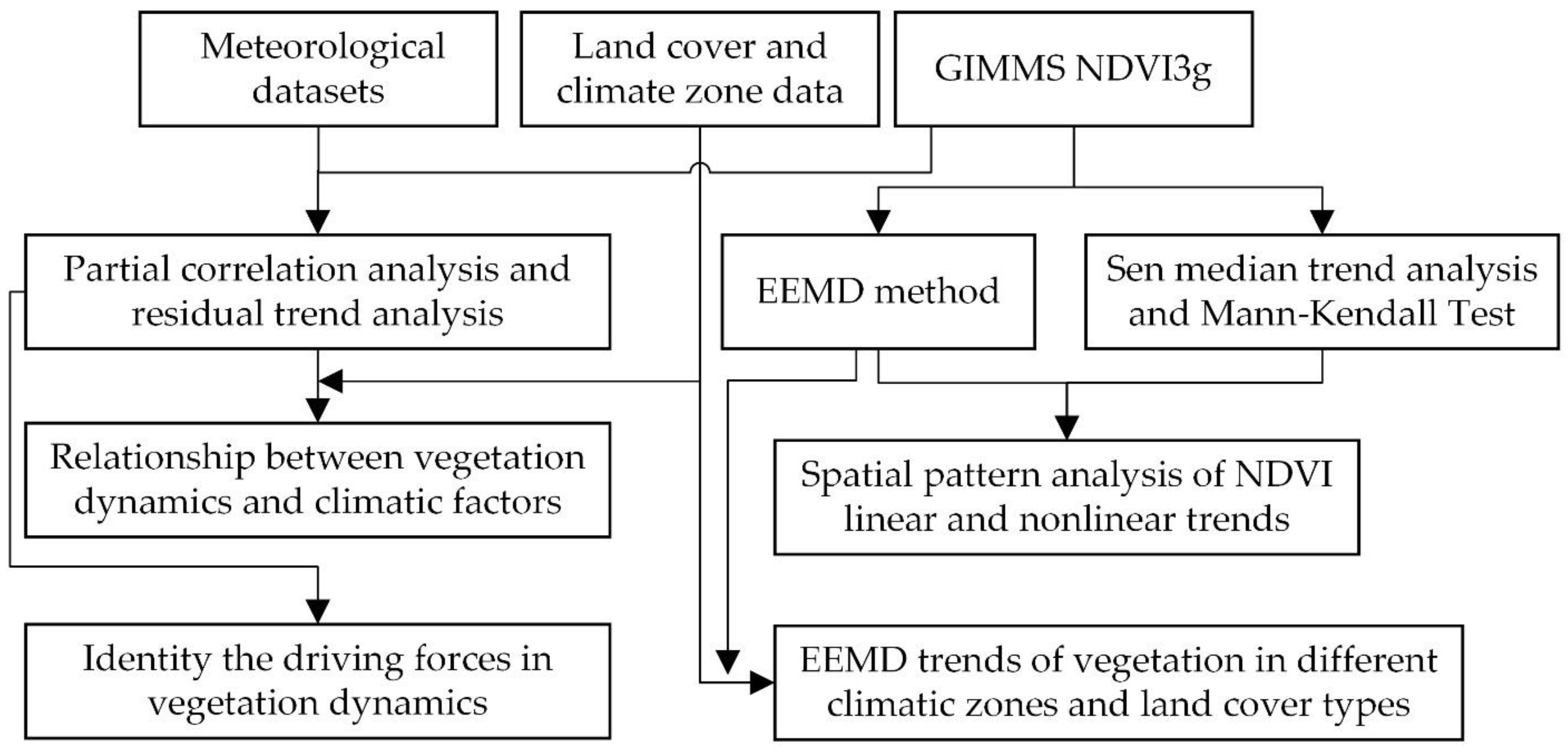
To better explain the overall process of this study, Figure 3 shows the flow chart.

3. Result

3.1. Temporal Variations of GSN from 1982 to 2015

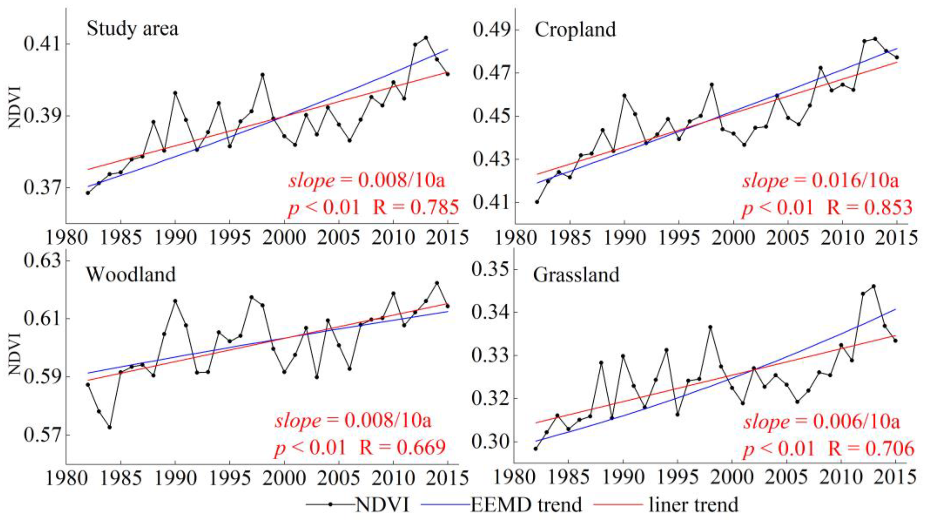
The linear trend showed that the average GSN fluctuated and increased significantly, with an average rate of 0.008/10a (p < 0.01) (Figure 4). Among them, the increasing rate of cropland GSN was the highest and that of grassland vegetation was the lowest, which were 0.016/10a (p < 0.01) and 0.006/10a (p < 0.01), respectively. According to EEMD method, GSN of all vegetation land also showed a significant increase trend (p < 0.05), and the change rate increased over time from 0.010/10a in 1983 to 0.013/10a in 2015. The EEMD trend of GSN of the three vegetation types increased significantly (p < 0.05), and the change rates of cropland and grassland increased over time, from 0.018/10a and 0.007/10a in 1983 to 0.020/10a and 0.012/10a in 2015, respectively, while the change rate of woodland decreased from 0.007/10a in 1983 to 0.006/10a in 2015. In order to compare with the linear trend, we calculated their average EEMD trend, which were 0.012/10a, 0.019/10a, 0.006/10a and 0.009/10a, respectively. The average EEMD trend of cropland and grassland was significantly higher than the linear trend, while that of woodland was the opposite. The EEMD trends of cropland and grassland in the later stage were higher than those in the earlier stage, indicating vegetation greenness accelerating, while the EEMD trend of woodland was decreasing, indicating slow vegetation greenness.

3.2. Spatial Pattern of Linear and Nonlinear Trends of GSN

Figure 5a,b show that the spatial distribution of high and low values of the change rate of Sen trend and average EEMD trend is relatively similar. The linear trend indicated that the area with a significant monotonic greening trend (G to G) was slightly larger than that with a non-significant trend (Non-sig), accounting for 47.69% and 46.55% of the total area, respectively. The area with a significant monotonic browning trend (B to B) was the lowest, accounting for only 5.76% (Figure 5c). The regions with a monotonic greening trend of GSN were mainly distributed in the WTSH, SH, PCA, and the southern MTA. The areas with a monotonic browning trend of vegetation were mainly concentrated in the northeastern and southwestern parts of the study area.
The area with vegetation monotonic trend (monotonic greening and monotonic browning) detected by EEMD accounted for 23.41% of the total area, of which the area with monotonic greening trend accounted for 22.29%, and the area with monotonic browning trend accounted for only 1.12%. According to EEMD, 36.64% of the region’s vegetation growth trend had shifted, of which 16.17% had changed from greening to browning, and 20.47% had changed from browning to greening. The areas with vegetation monotonic greening trend were mainly distributed in the southeastern and southern parts of the study area, while monotonic browning areas were small and scattered. The areas with greening to browning trend of vegetation mainly occurred in the northeastern, eastern, northwestern and southwestern parts of the study area. The areas with browning to greening trend were mainly distributed in the central and western parts of the study area and the northern of the plateau climate zone (Figure 5d).
Regardless of linear or nonlinear methods, the area with vegetation monotonic browning trend was the smallest, accounting for 1.12% and 5.76% of the total area, respectively (Table 3). Compared with EEMD method, the Mann–Kendall method can only distinguish three types (B to B, G to G and Non-sig), and it is impossible to judge whether there is a reversal trend of vegetation growth. For example, in the central and eastern regions of the study area, the results of the Mann–Kendall method showed a monotonic greening, while the trend obtained by EEMD method was from browning to greening and from greening to browning. The vegetation in about 30.70% of the study area showed a non-significant trend using the two methods, but the vegetation in 9.36%, 4.50%, 1.77% and 0.22% of the areas showed greening to browning trend, browning to greening trend, monotonic greening trend and monotonic browning trend for the EEMD method, while the Mann–Kendall method showed a non-significant change. About 20.52% of the vegetation in the study area showed a monotonic green trend for the two methods, but about 7.23%, 4.16% and 15.78% of the vegetation showed a non-significant trend, greening to browning trend and browning to greening trend for the EEMD method, while the Mann–Kendall method showed a significant monotonic greening trend. Only 0.90% of the vegetation in the study area showed monotonic browning trend for the two methods, but about 2.02%, 2.65% and 0.19% of the vegetation for the EEMD method was a non-significant trend, greening to browning trend and browning to greening trend, while the Mann–Kendall method showed a significant monotonic browning trend. The area percentage of monotonic greening trend for the Mann–Kendall method was much larger than that for the EEMD method, which was 47.69% and 22.29%, respectively (Table 3). The results showed that EEMD is necessary to analyze the actual evolution of vegetation and the deficiency of linear trend, while linear trend analysis underestimates the potential possibility of vegetation restoration or degradation.
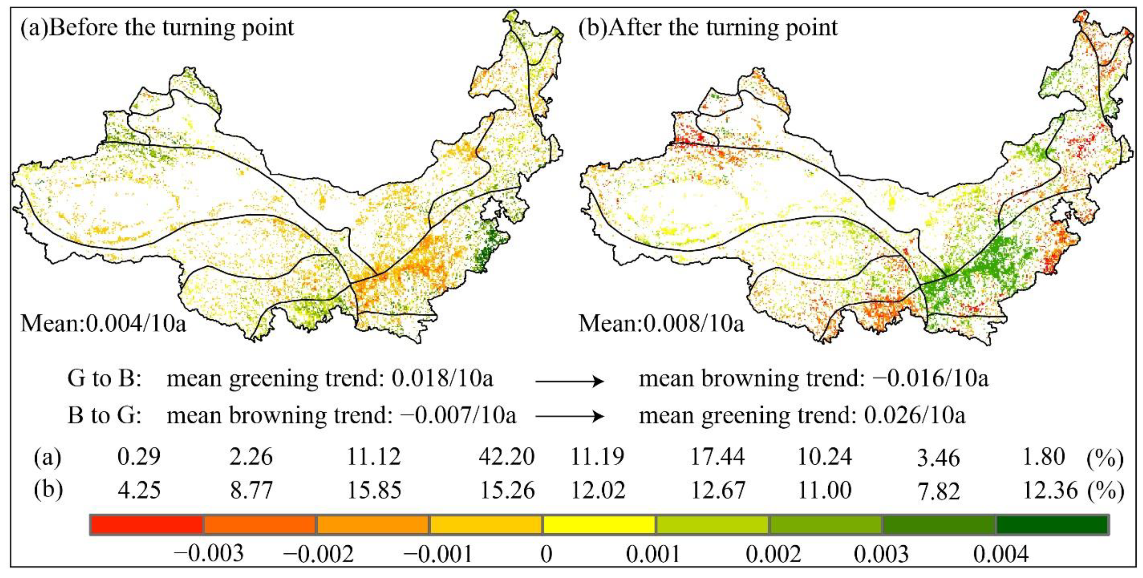
Based on EEMD, the TP of vegetation growth was obtained, which mainly occurred before 1995, accounting for 63.65% of the area with the reversal trend, especially before 1990, which accounted for 38.29%, mainly concentrated in the central part of the study area (Figure S1). The average EEMD trend of vegetation increased from 0.004/10a before the TP to 0.008/10a after the TP. The trend increased significantly, which was twice more than before the TP. Before the TP, the trend of vegetation degradation was mostly concentrated in the range of −0.001 to 0 (Figure 6). Before and after the TP, the browning to greening trend can be divided into monotonic browning and monotonic greening trend, and the greening to browning trend can be divided into monotonic greening and monotonic browning trend. The vegetation restoration trend was obvious, from −0.007/10a of browning trend to 0.026/10a of greening trend. Similarly, the risk of vegetation degradation was very high, from 0.018/10a of greening trend to −0.016a/10a of browning trend. After the TP, the vegetation growth and restoration effect in the central part of the study area was obvious and maintains a high greening trend, while the vegetation changed from a high greening trend to a high browning trend in the southwestern, northwestern, and northeastern parts of the study area, with a high risk of degradation (Figure 6). Therefore, it is necessary to pay more attention to the shift trend of vegetation and evaluate the degradation risk of different vegetation.

3.3. EEMD Trend of Vegetation in Different Climatic Zones and Land Cover

The cropland area with an increasing trend (monotonic greening and browning to greening) accounted for 56.67%, which was much higher than that with degradation or potential degradation trend (monotonic browning or greening to browning) (accounting for 19.20%) (Table 4). The vegetation of many croplands had changed from previous degradation to restoration. The trend of woodland was mainly non-significant, accounting for 42.44% in area. Among the significant trends, the monotonic greening area was the largest (23.06%), followed by greening to browning (20.63%). Similarly, the area of grassland with the non-significant trend accounted for 43.80%. Among the significant trends, the browning to greening area accounted for the largest (21.74%), followed by monotonic greening (18.84%). The areas of cropland, woodland and grassland with reverse trend were higher than that with monotonic trend, which accounted for 41.05% vs. 34.82%, 33.24% vs. 24.32%, 36.22% vs. 19.98%, respectively. The potential degradation risk of woodland was higher, followed by cropland (Table 4).
The cropland in SH, WTSH, WTA and MTSH showed an obvious increasing trend, accounting for 73.06%, 61.58%, 62.33% and 57.25% of the total cropland area in the corresponding climate zones, respectively (Table S1). The increasing trend of woodland in SH and WTSH was obvious, accounting for 54.70% and 63.54% of the total woodland area in the corresponding climate zone, respectively, of which the monotonic greening trend accounted for 44.16% and 44.52%, respectively. The area proportion of the woodland with the non-significant trend in CTH, MTSH and MTSA was higher than 50%, and the potential risk of vegetation degradation was high. The potential degradation risk of grassland in PCSH was the highest, followed by the CTH (the number of pixels in MTH was small and could be ignored), and the areas from greening to browning trend were 48.49% and 30.68%, respectively. Grassland had been significantly improved in MTA, WTSH, WTA, PCA and SH, accounting for 43.60%, 79.92%, 42.13%, 58.83% and 73.94% of the grassland area in the corresponding climate zones, respectively. Among them, the monotonic greening trend of grassland in WTSH and SH was 42.06% and 58.79, respectively, which was significantly better than that in other climatic zones.

3.4. Relationship between Vegetation Dynamics and Climate Factors

3.4.1. Correlation between Vegetation Dynamics with Reversal Trend and Climate Factors

The PCCs between GSN and GS-Tem, GS-Pre, and GS-SR were abbreviated as RTem, RPre and RSR, respectively. Before the TP, RTem, RPre and RSR were mainly positive correlation, accounting for 58.92%, 68.83% and 56.15%. The regions with RTem < 0 were mainly distributed in the northwestern WTSH and the southern MTA. Regions with RPre < 0 were mainly distributed in the southern part of plateau climate zone and central WTSH. The regions with RSR < 0 were mainly concentrated in the central MTA, the western PCSA, the western WTSH and the high altitude region (Figure 7a,c,e). After the TP, the area with RTem > 0 and RSR > 0 decreased from 58.92% to 50.47% and 56.15% to 52.48%, respectively, while the area with RPre > 0 increased slightly from 68.83% to 70.25%. Before and after the TP, the areas of RTem, RPre and RSR passing the significance test of p < 0.05 increased from 13.26%, 9.73% and 7.38% to 26.48%, 36.52% and 29.13%, respectively (Figure 7b,d,f).
Before and after the TP, the correlation between GSN and the three climate factors had changed significantly (Figure 7a–f). According to the square value of RTem, RPre and RSR, the dominant climate factors of vegetation growth were obtained (Figure 7g,h). Before the TP, the temperature-dominated area accounted for 39.34%, followed by precipitation (34.78%). After the TP, vegetation growth was mainly controlled by precipitation (43.70%), and the area controlled by solar radiation (28.83%) was slightly higher than that controlled by temperature (27.47%). The performance of different type vegetation was slightly different. Before the TP, cropland and grassland was mainly affected by temperature (38.57% and 39.11%), followed by precipitation (35.38% and 37.09%), while woodland was mainly affected by temperature and solar radiation (41.49% and 34.88%) (Table 5). After the TP, precipitation became the dominant factor, accounting for 48.41% and 43.40% of cropland and grassland, and the effects of temperature and solar radiation on cropland and grassland were close. The woodland was mainly affected by precipitation and solar radiation (38.39% and 36.34%), and there was little difference in the percentage of their dominant area (Table 5). The climate dominant factor of vegetation growth changed from temperature to precipitation in the northwestern WTSH and the central and southern MTA, while from temperature to solar radiation in PCSH. The correlation between vegetation and climate factors reversed or increased before and after the TP, indicating that the response of vegetation to climate change shifted after the TP.

3.4.2. Correlations between Vegetation Dynamics with Monotonic Trend and Non-Significant Trend and Climate Factors

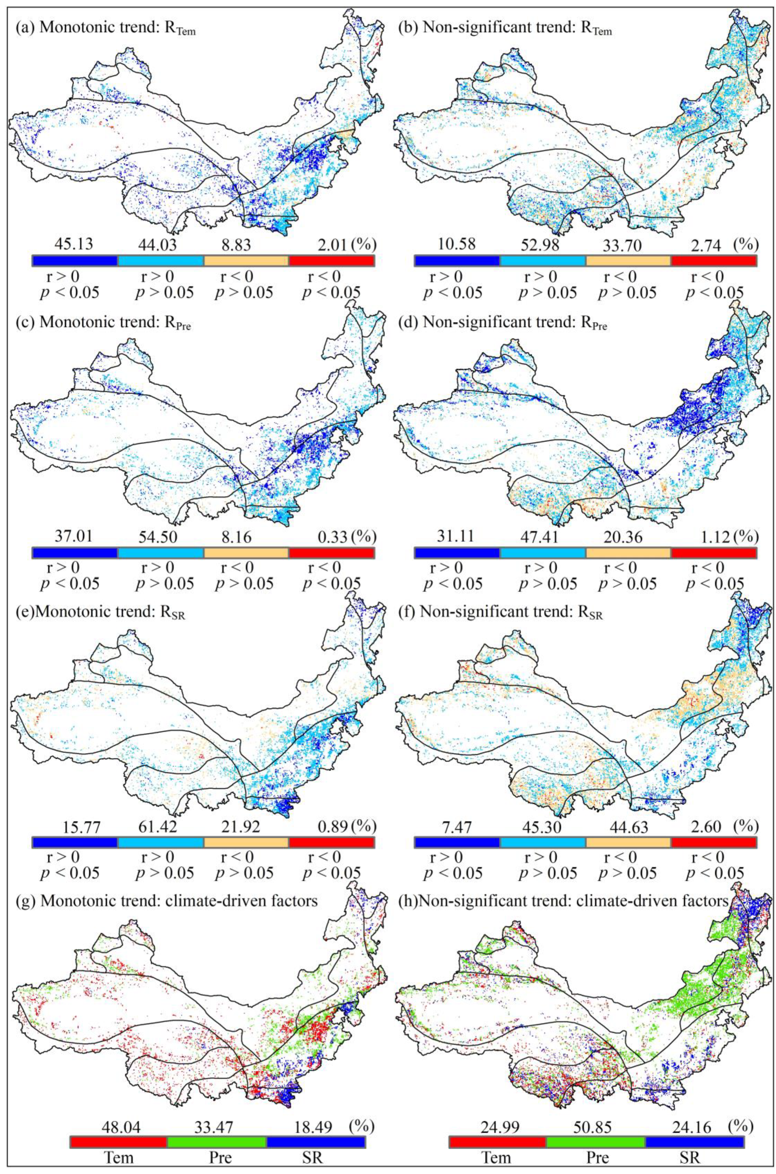
The GSN with monotonic trend was mainly positively correlated with GS-Tem, GS-Pre and GS-SR with 89.16%, 91.51% and 77.19% the area percentage (Figure 8a,c,e). The area with significant positive correlation between GSN and GS-Tem was slightly higher than that with non-significant positive correlation (Figure 8a). The areas with significant positive correlation between GSN and GS-Pre and GS-SR accounted for 37.01% and 15.77%, respectively (Figure 8c,e). The vegetation growth in the northern and western regions of WTSH, the WTA and plateau climate area was mainly controlled by temperature. Vegetation growth was mainly affected by precipitation in the northwestern part of WTSH and the southern part of MTA. The vegetation growth dominated by solar radiation was mainly distributed in the eastern part of SH, southern of WTSH and CTH (Figure 8g). The significant positive correlation area between NDVI and temperature was higher than that of precipitation and solar radiation. Overall, the vegetation growth with monotonic trend was mainly controlled by temperature, accounting for 48.04% of the study area, followed by precipitation (33.47%) (Figure 8g). The order of main climatic factors affecting cropland and grassland was consistent with the overall vegetation, while woodland was mainly affected by solar radiation (41.04%), followed by temperature (36.12%) (Table 5).
The GSN with non-significant trend was positively correlated with GS-Tem, GS-Pre and GS-SR, accounting for 63.56%, 78.52% and 52.77%, respectively (Figure 8b,d,f). The area with significant positive correlation between GSN and GS-Pre accounted for 31.11%, which was much higher than that between GS-Tem and GS-SR (10.58% and 7.47%, respectively). The regions with significant RPre > 0 were mainly distributed in MTSA and MTA. The regions with significant RSR > 0 were mainly concentrated in the northeastern and southeastern parts of the study area (Figure 8b,d,f). The vegetation with non-significant trend was mainly controlled by precipitation (accounting for 50.85%), which was mainly distributed in arid and semi-arid areas. The vegetation in the plateau climate area was mainly controlled by temperature, while the vegetation dominated by solar radiation was mainly concentrated in the northeastern and southeastern parts of the study area (Figure 8h). Similarly, the impact of precipitation on cropland and grassland was larger than solar radiation and temperature, while solar radiation had the greatest impact on woodland, followed by precipitation (Table 5).

3.5. Identity the Driving Forces in Vegetation Dynamics

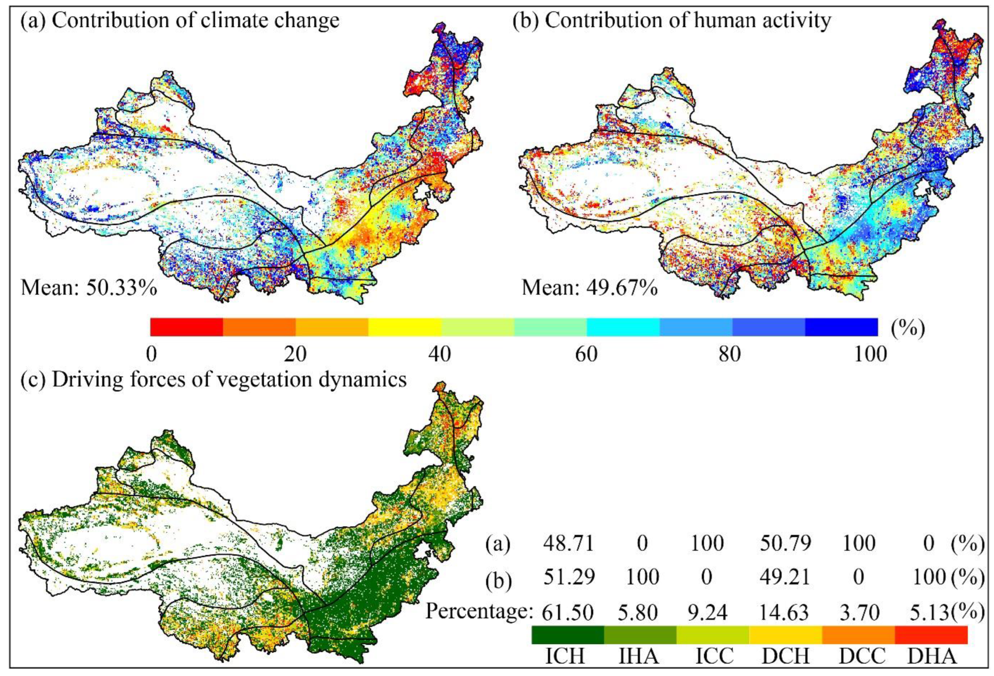
Climate change and human activities were conducive to the vegetation growth in most areas, accounting for 76.54% of the total area (Figure 9). A total of 61.50% of the vegetation restoration in the study area was affected by the interaction of climate change and human activities (ICH), of which the average contribution of climate change and human activities to ICH was 48.71% and 51.29%, respectively (Figure 9). ICH-induced vegetation restoration was mainly concentrated in the central, southeastern, southern and western parts of the study area. IHA-induced vegetation restoration was mainly distributed in MTSA, accounting for 5.80% of the study area. However, 9.24% of the area was only affected by ICC, which was distributed in CTH, PCSH and PCSA. The vegetation on 23.46% of the study area had degraded, which was mainly distributed in the northeastern, southwestern and northwestern parts of the study area. DCH was the main driving force of vegetation degradation, accounting for 14.63% of the total area, followed by DHA (5.13%) and DCC (3.70%). The average contribution of climate change and human activities to DCH was 50.79% and 49.21%, respectively (Figure 9).
On the whole, the average contributions of climate change and human activities were 50.33% and 49.67%, with 51.22% and 48.78% for the vegetation restoration area, and 47.53% and 52.57% for the vegetation degradation area, respectively (Table 6). In general, climate change was the dominant factor in the vegetation restoration area, and human activities were the main driving force in the vegetation degradation area, but the dominant factors of different types of vegetation were significantly different. In the vegetation restoration area, the growth of woodland and grassland was mainly controlled by climatic factors, while the cropland was mainly affected by human activities. In the vegetation degradation area, human activities were the main factors of leading woodland and grassland to degrade, while cropland was mainly controlled by climatic factors. Overall, the contribution of climate change to the dynamics of woodland and grassland was higher than that of human activities, and the contribution of human activities to the dynamics of cropland was much higher than that of climate change (Table 6). The dominant factors of vegetation restoration and degradation had significant spatial heterogeneity (Figure 9a,b). The contribution of human activities was significantly higher than that of climate change in the southeastern part of the study area, while it is generally lower than that of climate change in the western and northwestern parts of the study area.

4. Discussion

This study showed that the trend of NDVI has an increasing rate over time for the EEMD method (Figure 4), which indicated that the process of vegetation was not linear, but nonlinear and variable [10]. Due to its simplicity and convenience, linear trend analysis is still used by many researchers [14,44]. However, linear trend analysis can only obtain the average change rate of vegetation during the study period, and judge the type of change trend [10]. It is easy to underestimate or overestimate the potential risk of vegetation restoration or degradation [12]. The long-term trend obtained by EEMD reveals the change process and trend of vegetation growth over time [23], and has been applied in many studies [6,23,42].
This study showed that the TP of vegetation from browning to greening happened in the early 1990s, which was consistent with the results of Xu et al. [23], while the time of vegetation growth from greening to browning in high altitude areas, such as the southern of the plateau climate zone and the northwestern of the study area, the eastern WTSH, and the CTH was usually later than that in other greening to browning areas (Figure S1). The TP of vegetation has obvious geographical heterogeneity. However, some researchers obtained one or two turning points based on a piecewise linear regression method [45,46] for large-scale regional vegetation change analysis, which will not accurately reflect the real situation of vegetation change. In addition, the vegetation growth trend in Central Asia, Eastern Europe and East Africa [10,12,47,48] had also been reversed on a large scale, which may provide early warning for ecosystem changes under global environmental change [23]; therefore, researchers should pay more attention.
The vegetation in the high altitude area in the northwestern and southwestern parts of the study area experienced a trend transfer process from greening to browning (Figure 5 and Figure 6), which was the same as Liu’s research results [30], but not consistent with the increasing trend considered by other researchers using linear trend analysis [49,50]. From 1982 to 2015, the temperature and solar radiation showed an increasing trend, while the precipitation changed from decreasing to increasing (Figure S2). When the temperature rises, the snow on the mountain will melt, which increases the surface runoff and soil moisture [51,52,53]. In addition, the increase of temperature can improve the root activity of vegetation, improve the photosynthesis rate of vegetation, and contribute to the growth of vegetation [54]. However, the rapid rise in temperature may promote vegetation transpiration, thus accelerating soil water loss [55]. When forced by soil water, vegetation photosynthesis will slow down, which then depresses the growth of vegetation [56]. In addition, the increase in precipitation in high altitude areas means the shortage of sunshine time and the reduction in solar radiation, and the photosynthesis of vegetation will also be suppressed, which is not conducive to the growth of vegetation [57,58]. On the other hand, human activities, such as excessive grassland grazing, are also an important contributor to the vegetation growth trend from greening to browning [59,60]. The vegetation in the central part of the study area, especially the Loess Plateau, had experienced a process from browning trend to greening trend (Figure 5 and Figure 6), which was closely related to ecological projects implemented in China, such as Natural Forest Conservation Program, Grain for Green Program and grazing management, which can promote the significant increase in vegetation coverage [61]. In the early stage, the increase in temperature and solar radiation and the decrease in precipitation triggered the degradation of vegetation in central Inner Mongolia [36]. However, in the later period, the increase in precipitation and the implementation of the Beijing-Tianjin Sand Source Control Program effectively resisted the adverse impact of climate, and promoted the reversal of vegetation growth trend from browning to greening [36,45].
According to different geographical locations and vegetation types, climate change and human activities play different roles in vegetation dynamics [60]. The change rate of cropland is significantly higher than that of woodland and grassland (Figure 4), with cropland generally being distributed in low altitude areas (Figure 1). Therefore, it is highly affected by human activities, such as artificial irrigation, application of chemical fertilizer, and change of planting structure or varieties, which are conducive to vegetation greening [58]. However, the cropland located in the northeastern part of WTSH has a high potential degradation risk (Figure 5 and Figure 6), which may be related to the population increase and the rapid development of urbanization in this area [58]. In the CTH, MTSH and MTSA climate zones, woodland was accompanied by a high potential degradation risk (Table S1). The woodland in CTH was mainly affected by temperature and solar radiation, while in MTSH and MTSA, it was mainly affected by temperature and precipitation [36]. From 1990 to 2006, temperature and solar radiation showed increasing trends, while the precipitation showed a decreasing trend, while from 2006 to 2015, the trend was opposite [36]. The growth of woodland in arid and semi-arid areas requires significantly higher water conditions than that in humid climate areas, so the potential degradation risk of woodland may be caused by adverse factors of climate conditions. In addition, the rapid development of social economy and more urban construction activities may seriously damage the ecological environment, reduce the vegetation coverage, and lead to vegetation degradation [45,62].
The geographical difference of grassland change trend was obvious (Figure 5). Adverse factors of climate change and unreasonable human activities, such as long-term overgrazing, have reduced the self-recovery ability of grassland vegetation and caused the degradation of most natural grasslands to varying degrees [63,64], which seriously affects the sustainable development of grassland animal husbandry and the stability and development of economic and social in pastoral areas. However, favorable climatic conditions and reasonable ecological restoration measures, such as reducing grazing intensity and extending the restoration time of pasture, can effectively improve vegetation productivity and promote vegetation restoration [65]. In addition, human activities can also play a positive role in vegetation restoration under adverse climatic conditions [45]. Therefore, active human intervention and measures can promote the restoration of degraded ecosystems and promote regional sustainable development [66].
The methods used in this study have been widely recognized [12,41,44], but there are still some shortcomings. GIMMS NDVI3g data with 8km spatial resolution cannot reflect more detailed spatial information, and it is difficult to reflect the changes of local vegetation within the pixel scale. Therefore, the NDVI products with higher spatial resolution should be used in future study. Because of the difference in geographical location, the response of vegetation to climate factors has different lag effects [43]. Therefore, in future studies, the lag effects between vegetation and climate factors will be considered in order to improve the accuracy of assessment [41]. In the study, climate factors only selected temperature, precipitation and solar radiation, ignoring the impact of other factors on vegetation change, such as CO2 [67], nitrogen deposition [68], and soil moisture [69]. The interactive effect of temperature, precipitation and solar radiation is also not considered in this study. In addition, extreme climate events have a great impact on different ecosystems, and the impact on vegetation changes shows regional diversity [70,71]. Therefore, more climate factors will be considered to analyze the impact of climate change on vegetation change, which will help comprehensively understand the relationship between vegetation and climate, and more accurately assess the contribution of human activities to vegetation change. At present, human activities are analyzed as a whole, and how to quantitatively evaluate the impact of different types of human activities on vegetation change is still an important issue [72].

5. Conclusions

This study analyzed the linear and nonlinear trends of vegetation in northern China from 1982 to 2015, assessed the response of different types of vegetation to climate change, and quantified the relative impact of climate change and human activities on vegetation change. The results show that the vegetation in most areas has undergone significant changes during the whole study period. The vegetation growth in 36.64% of the areas had a reverse trend. There were potential risks of vegetation degradation in the southwestern, northwestern and northeastern parts of the study area. The potential degradation risk of woodland was higher than that of cropland and grassland vegetation.
The correlation between vegetation and climate factors was reversed or enhanced before and after the turning point. Temperature and precipitation were the main climatic factors affecting the vegetation with a monotonic trend, and precipitation dominated the vegetation with a non-significant trend. The areas affected by temperature were mainly located in high altitude areas, arid and sub-arid areas were mainly affected by precipitation, and humid and sub-humid areas were mainly affected by solar radiation.
Climate change and human activities had promoted vegetation growth in 76.54% of the study area. Overall, the average contribution rates of climate change and human activities to vegetation change were 50.33% and 49.67%, respectively. The vegetation restoration of grassland and woodland was mainly dominated by climate change, and human activities mainly dominated the vegetation degradation, while the cropland vegetation had the opposite performance. The contribution rate of human activities to the vegetation change in the southeastern and eastern parts of the study area was generally higher than that of climate change, but it was opposite in the higher altitude area, with obvious spatial heterogeneity. The results are helpful to understand the dynamic changes of vegetation in northern China, and provide important reference value for regional ecological protection and restoration.

Supplementary Materials

The following are available online at https://www.mdpi.com/article/10.3390/rs14236163/s1, Figure S1: the timing of the turning points of NDVI in growing season with EEMD method (p < 0.05). Figure S2: EEMD long-term trend of temperature, precipitation and solar radiation in the study area from 1982 to 2015. Table S1: statistical proportion of NDVI EEMD trend in vegetation growing season under different climatic zones (%).

Author Contributions

R.S. processed the data, analyzed the results, and wrote the manuscript. R.S., S.C. and H.S. revised the manuscript. All authors have read and agreed to the published version of the manuscript.

Funding

The research is jointly supported by the National Key Research and Development Program of China (2021YFC3201102), the National Natural Science Foundation of China (U2003105), the Second Tibetan Plateau Scientific Expedition and Research Program (2019QZKK1003), and the Strategic Priority Research Program A of the Chinese Academy of Sciences (XDA20010301).

Data Availability Statement

Not applicable.

Acknowledgments

The authors thank the GIMMS group for providing the GIMMS NDVI3g data, the China Meteorological Data Service Center for providing the climate station data, the European Centre for Medium-Range Weather Forecasts for providing the monthly solar radiation data, and the Data Center for Resources and Environmental Sciences, Chinese Academy of Sciences, for providing the land cover and climate zone data.

Conflicts of Interest

The authors declare no conflict of interest.

References

  1. Fu, B.; Wang, S.; Liu, Y.; Liu, J.; Liang, W.; Miao, C. Hydrogeomorphic Ecosystem Responses to Natural and Anthropogenic Changes in the Loess Plateau of China. Annu. Rev. Earth Planet. Sci. 2017, 45, 223–243. [Google Scholar] [CrossRef]
  2. Ding, Z.; Peng, J.; Qiu, S.; Zhao, Y. Nearly Half of Global Vegetated Area Experienced Inconsistent Vegetation Growth in Terms of Greenness, Cover, and Productivity. Earths Future 2020, 8, e2020EF001618. [Google Scholar] [CrossRef]
  3. Hua, W.; Chen, H.; Zhou, L.; Xie, Z.; Qin, M.; Li, X.; Ma, H.; Huang, Q.; Sun, S. Observational Quantification of Climatic and Human Influences on Vegetation Greening in China. Remote Sens. 2017, 9, 425. [Google Scholar] [CrossRef] [Green Version]
  4. Wang, J.; Wang, K.; Zhang, M.; Zhang, C. Impacts of climate change and human activities on vegetation cover in hilly southern China. Ecol. Eng. 2015, 81, 451–461. [Google Scholar] [CrossRef]
  5. Xie, B.; Jia, X.; Qin, Z.; Shen, J.; Chang, Q. Vegetation dynamics and climate change on the Loess Plateau, China: 1982–2011. Reg. Environ. Chang. 2016, 16, 1583–1594. [Google Scholar] [CrossRef]
  6. Liu, H.; Zhang, M.; Lin, Z.; Xu, X. Spatial heterogeneity of the relationship between vegetation dynamics and climate change and their driving forces at multiple time scales in Southwest China. Agric. For. Meteorol. 2018, 256, 10–21. [Google Scholar] [CrossRef]
  7. Xue, Y.; Zhang, B.; He, C.; Shao, R. Detecting Vegetation Variations and Main Drivers over the Agropastoral Ecotone of Northern China through the Ensemble Empirical Mode Decomposition Method. Remote Sens. 2019, 11, 1860. [Google Scholar] [CrossRef] [Green Version]
  8. Sun, R.; Chen, S.; Su, H. Spatiotemporal variations of NDVI of different land cover types on the Loess Plateau from 2000 to 2016. Prog. Geogr. 2019, 38, 1248–1258. [Google Scholar] [CrossRef] [Green Version]
  9. Hu, M.; Xia, B. A significant increase in the normalized difference vegetation index during the rapid economic development in the Pearl River Delta of China. Land Degrad. Dev. 2019, 30, 359–370. [Google Scholar] [CrossRef]
  10. Wei, F.; Wang, S.; Fu, B.; Pan, N.; Feng, X.; Zhao, W.; Wang, C. Vegetation dynamic trends and the main drivers detected using the ensemble empirical mode decomposition method in East Africa. Land Degrad. Dev. 2018, 29, 2542–2553. [Google Scholar] [CrossRef]
  11. Bhavani, P.; Roy, P.S.; Chakravarthi, V.; Kanawade, V.P. Satellite Remote Sensing for Monitoring Agriculture Growth and Agricultural Drought Vulnerability Using Long-Term (1982–2015) Climate Variability and Socio-economic Data set. Proc. Natl. Acad. Sci. India Sect. A-Phys. Sci. 2017, 87, 733–750. [Google Scholar] [CrossRef]
  12. Pan, N.; Feng, X.; Fu, B.; Wang, S.; Ji, F.; Pan, S. Increasing global vegetation browning hidden in overall vegetation greening: Insights from time-varying trends. Remote Sens. Environ. 2018, 214, 59–72. [Google Scholar] [CrossRef]
  13. Liu, Z.; Qiu, B.; Wang, Z.; Qi, W. Temporal and spatial variation analysis of vegetation cover in the Loess Plateau from 2001 to 2014. Remote Sens. Land Resour. 2017, 29, 192–198. [Google Scholar]
  14. Jiang, H.; Xu, X.; Guan, M.; Wang, L.; Huang, Y.; Jiang, Y. Determining the contributions of climate change and human activities to vegetation dynamics in agro-pastural transitional zone of northern China from 2000 to 2015. Sci. Total Environ. 2020, 718, 134871. [Google Scholar] [CrossRef] [PubMed]
  15. Zhang, Y.; Peng, C.; Li, W.; Tian, L.; Zhu, Q.; Chen, H.; Fang, X.; Zhang, G.; Liu, G.; Mu, X.; et al. Multiple afforestation programs accelerate the greenness in the “Three North” region of China from 1982 to 2013. Ecol. Indic. 2016, 61, 404–412. [Google Scholar] [CrossRef]
  16. Yang, X.; Xu, B.; Jin, Y.; Qin, Z.; Ma, H.; Li, J.; Zhao, F.; Chen, S.; Zhu, X. Remote sensing monitoring of grassland vegetation growth in the Beijing-Tianjin sandstorm source project area from 2000 to 2010. Ecol. Indic. 2015, 51, 244–251. [Google Scholar] [CrossRef]
  17. Feng, X.; Fu, B.; Lu, N.; Zeng, Y.; Wu, B. How ecological restoration alters ecosystem services: An analysis of carbon sequestration in China’s Loess Plateau. Sci. Rep. 2013, 3, 2846. [Google Scholar] [CrossRef] [Green Version]
  18. Xu, G.; Zhang, J.; Li, P.; Li, Z.; Lu, K.; Wang, X.; Wang, F.; Cheng, Y.; Wang, B. Vegetation restoration projects and their influence on runoff and sediment in China. Ecol. Indic. 2018, 95, 233–241. [Google Scholar] [CrossRef]
  19. Pinzon, J.E.; Tucker, C.J. A Non-Stationary 1981–2012 AVHRR NDVI3g Time Series. Remote Sens. 2014, 6, 6929–6960. [Google Scholar] [CrossRef] [Green Version]
  20. Jiang, N.; Zhu, W.; Zheng, Z.; Chen, G.; Fan, D. A Comparative Analysis between GIMSS NDVIg and NDVI3g for Monitoring Vegetation Activity Change in the Northern Hemisphere during 1982–2008. Remote Sens. 2013, 5, 4031–4044. [Google Scholar] [CrossRef] [Green Version]
  21. Verbesselt, J.; Hyndman, R.; Newnham, G.; Culvenor, D. Detecting trend and seasonal changes in satellite image time series. Remote Sens. Environ. 2010, 114, 106–115. [Google Scholar] [CrossRef]
  22. Jamali, S.; Jonsson, P.; Eklundh, L.; Ardo, J.; Seaquist, J. Detecting changes in vegetation trends using time series segmentation. Remote Sens. Environ. 2015, 156, 182–195. [Google Scholar] [CrossRef]
  23. Xu, X.; Liu, H.; Jiao, F.; Gong, H.; Lin, Z. Time-varying trends of vegetation change and their driving forces during 1981-2016 along the silk road economic belt. Catena 2020, 195, 104796. [Google Scholar] [CrossRef]
  24. Wu, Z.; Huang, N.E. Ensemble Empirical Mode Decomposition: A Noise-Assisted Data Analysis Method. Adv. Data Sci. Adapt. Anal. 2009, 1, 1–41. [Google Scholar] [CrossRef]
  25. Sun, H.M.; Cheng, J.; Ma, Z. An EEG signal denoising method based on ensemble empirical mode decomposition and independent component analysis. In Proceedings of the IEEE International Conference on Cyborg and Bionic Systems (CBS), Shenzhen, China, 25–27 October 2018; pp. 401–405. [Google Scholar]
  26. Shi, F.; Yang, B.; von Gunten, L.; Qin, C.; Wang, Z. Ensemble empirical mode decomposition for tree-ring climate reconstructions. Theor. Appl. Climatol. 2012, 109, 233–243. [Google Scholar] [CrossRef]
  27. Wang, W.C.; Chau, K.W.; Xu, D.M.; Chen, X.Y. Improving Forecasting Accuracy of Annual Runoff Time Series Using ARIMA Based on EEMD Decomposition. Water Resour. Manag. 2015, 29, 2655–2675. [Google Scholar] [CrossRef]
  28. Chen, T.; Tang, G.; Yuan, Y.; Guo, H.; Xu, Z.; Jiang, G.; Chen, X. Unraveling the relative impacts of climate change and human activities on grassland productivity in Central Asia over last three decades. Sci. Total Environ. 2020, 743, 140649. [Google Scholar] [CrossRef]
  29. Jiao, F.; Liu, H.; Xu, X.; Gong, H.; Lin, Z. Trend Evolution of Vegetation Phenology in China during the Period of 1981-2016. Remote Sens. 2020, 12, 572. [Google Scholar] [CrossRef] [Green Version]
  30. Liu, H.; Cao, L.; Jia, J.; Gong, H.; Qi, X.; Xu, X. Effects of land use changes on the nonlinear trends of net primary productivity in arid and semiarid areas, China. Land Degrad. Dev. 2021, 32, 2183–2196. [Google Scholar] [CrossRef]
  31. Liu, X.; Wu, Z.; Liu, Y.; Zhao, X.; Rui, Y.; Zhang, J. Spatial-temporal characteristics of precipitation from 1960 to 2015 in the Three Rivers’ Headstream Region, Qinghai, China. Acta Geogr. Sin. 2019, 74, 1803–1820. [Google Scholar]
  32. Jingyun, Z.; Yunhe, Y.I.N.; Bingyuan, L.I. A New Scheme for Climate Regionalization in China. Acta Geogr. Sin. 2010, 65, 3–12. [Google Scholar]
  33. Zhang, W.; Wang, L.; Xiang, F.; Qin, W.; Jiang, W. Vegetation dynamics and the relations with climate change at multiple time scales in the Yangtze River and Yellow River Basin, China. Ecol. Indic. 2020, 110, 105892. [Google Scholar] [CrossRef]
  34. Cao, R.; Chen, Y.; Shen, M.; Chen, J.; Zhou, J.; Wang, C.; Yang, W. A simple method to improve the quality of NDVI time-series data by integrating spatiotemporal information with the Savitzky-Golay filter. Remote Sens. Environ. 2018, 217, 244–257. [Google Scholar] [CrossRef]
  35. Holben, B.N. Characteristics of Maximum-Value Composite Images from Temporal Avhrr Data. Int. J. Remote Sens. 1986, 7, 1417–1434. [Google Scholar] [CrossRef]
  36. Sun, R.; Chen, S.; Su, H. Climate Dynamics of the Spatiotemporal Changes of Vegetation NDVI in Northern China from 1982 to 2015. Remote Sens. 2021, 13, 187. [Google Scholar] [CrossRef]
  37. Hutchinson, M.F. Interpolating Mean Rainfall Using Thin-Plate Smoothing Splines. Int. J. Geogr. Inf. Syst. 1995, 9, 385–403. [Google Scholar] [CrossRef]
  38. Liu, J.; Kuang, W.; Zhang, Z.; Xu, X.; Qin, Y.; Ning, J.; Zhou, W.; Zhang, S.; Li, R.; Yan, C.; et al. Spatiotemporal characteristics, patterns and causes of land use changes in China since the late 1980s. Acta Geogr. Sin. 2014, 69, 3–14. [Google Scholar] [CrossRef]
  39. Qu, S.; Wang, L.; Lin, A.; Zhu, H.; Yuan, M. What drives the vegetation restoration in Yangtze River basin, China: Climate change or anthropogenic factors? Ecol. Indic. 2018, 90, 438–450. [Google Scholar] [CrossRef]
  40. Yang, L.; Shen, F.; Zhang, L.; Cai, Y.; Yi, F.; Zhou, C. Quantifying influences of natural and anthropogenic factors on vegetation changes using structural equation modeling: A case study in Jiangsu Province, China. J. Clean. Prod. 2021, 280, 124330. [Google Scholar] [CrossRef]
  41. Peng, Q.; Wang, R.; Jiang, Y.; Li, C. Contributions of climate change and human activities to vegetation dynamics in Qilian Mountain National Park, northwest China. Glob. Ecol. Conserv. 2021, 32, e01947. [Google Scholar] [CrossRef]
  42. Gao, X.; Huang, X.; Lo, K.; Dang, Q.; Wen, R. Vegetation responses to climate change in the Qilian Mountain Nature Reserve, Northwest China. Glob. Ecol. Conserv. 2021, 28, e01698. [Google Scholar] [CrossRef]
  43. Wu, D.; Zhao, X.; Liang, S.; Zhou, T.; Huang, K.; Tang, B.; Zhao, W. Time-lag effects of global vegetation responses to climate change. Glob. Chang. Biol. 2015, 21, 3520–3531. [Google Scholar] [CrossRef]
  44. Zhao, C.; Yan, Y.; Ma, W.; Shang, X.; Chen, J.; Rong, Y.; Xie, T.; Quan, Y. RESTREND-based assessment of factors affecting vegetation dynamics on the Mongolian Plateau. Ecol. Model. 2021, 440, 109415. [Google Scholar] [CrossRef]
  45. Yu, L.; Wu, Z.; Du, Z.; Zhang, H.; Liu, Y. Insights on the roles of climate and human activities to vegetation degradation and restoration in Beijing-Tianjin sandstorm source region. Ecol. Eng. 2021, 159, 106105. [Google Scholar] [CrossRef]
  46. Kong, D.; Zhang, Q.; Singh, V.P.; Shi, P. Seasonal vegetation response to climate change in the Northern Hemisphere (1982-2013). Glob. Planet. Chang. 2017, 148, 1–8. [Google Scholar] [CrossRef] [Green Version]
  47. Li, Z.; Chen, Y.; Li, W.; Deng, H.; Fang, G. Potential impacts of climate change on vegetation dynamics in Central Asia. J. Geophys. Res. -Atmos. 2015, 120, 12345–12356. [Google Scholar] [CrossRef]
  48. de Jong, R.; Verbesselt, J.; Zeileis, A.; Schaepman, M.E. Shifts in Global Vegetation Activity Trends. Remote Sens. 2013, 5, 1117–1133. [Google Scholar] [CrossRef] [Green Version]
  49. Liu, Y.; Li, C.; Liu, Z.; Deng, X. Assessment of spatio-temporal variations in vegetation cover in Xinjiang from 1982 to 2013 based on GIMMS-NDVI. Acta Ecol. Sin. 2016, 36, 6198–6208. [Google Scholar]
  50. Dai, S.; Zhang, B.; Wang, H. Spatio-temporal Change of Vegetation Index NDVI in Northwest China and Its Influencing Factors. J. Geo-Inf. Sci. 2010, 12, 315–321. [Google Scholar] [CrossRef]
  51. He, B.; Chen, A.; Wang, H.; Wang, Q. Dynamic Response of Satellite-Derived Vegetation Growth to Climate Change in the Three North Shelter Forest Region in China. Remote Sens. 2015, 7, 9998–10016. [Google Scholar] [CrossRef] [Green Version]
  52. Zhu, Y.; Zhang, J.; Zhang, Y.; Qin, S.; Shao, Y.; Gao, Y. Responses of vegetation to climatic variations in the desert region of northern China. Catena 2019, 175, 27–36. [Google Scholar] [CrossRef]
  53. Li, H.; Liu, L.; Liu, X.; Li, X.; Xu, Z. Greening Implication Inferred from Vegetation Dynamics Interacted with Climate Change and Human Activities over the Southeast Qinghai-Tibet Plateau. Remote Sens. 2019, 11, 2421. [Google Scholar] [CrossRef] [Green Version]
  54. Jeong, S.-J.; Ho, C.-H.; Gim, H.-J.; Brown, M.E. Phenology shifts at start vs. end of growing season in temperate vegetation over the Northern Hemisphere for the period 1982–2008. Glob. Chang. Biol. 2011, 17, 2385–2399. [Google Scholar] [CrossRef]
  55. Yuan, X.; Hamdi, R.; Ochege, F.U.; Kurban, A.; De Maeyer, P. The sensitivity of global surface air temperature to vegetation greenness. Int. J. Climatol. 2021, 41, 483–496. [Google Scholar] [CrossRef]
  56. Jiao, K.; Gao, J.; Wu, S. Climatic determinants impacting the distribution of greenness in China: Regional differentiation and spatial variability. Int. J. Biometeorol. 2019, 63, 523–533. [Google Scholar] [CrossRef]
  57. Gottfried, M.; Pauli, H.; Futschik, A.; Akhalkatsi, M.; Barancok, P.; Benito Alonso, J.L.; Coldea, G.; Dick, J.; Erschbamer, B.; Fernandez Calzado, M.R.; et al. Continent-wide response of mountain vegetation to climate change. Nat. Clim. Chang. 2012, 2, 111–115. [Google Scholar] [CrossRef]
  58. Sun, R.; Chen, S.; Su, H. Spatiotemporal variation of NDVI in different ecotypes on the Loess Plateau and its response to climate change. Geogr. Res. 2020, 39, 1200–1214. [Google Scholar]
  59. Zhao, W.Y.; Li, J.L.; Qi, J.G. Changes in vegetation diversity and structure in response to heavy grazing pressure in the northern Tianshan Mountains, China. J. Arid Environ. 2007, 68, 465–479. [Google Scholar] [CrossRef]
  60. Wang, Z.; Zhang, Y.; Yang, Y.; Zhou, W.; Gang, C.; Zhang, Y.; Li, J.; An, R.; Wang, K.; Odeh, I.; et al. Quantitative assess the driving forces on the grassland degradation in the Qinghai-Tibet Plateau, in China. Ecol. Inform. 2016, 33, 32–44. [Google Scholar] [CrossRef]
  61. Li, G.; Sun, S.; Han, J.; Yan, J.; Liu, W.; Wei, Y.; Lu, N.; Sun, Y. Impacts of Chinese Grain for Green program and climate change on vegetation in the Loess Plateau during 1982–2015. Sci. Total Environ. 2019, 660, 177–187. [Google Scholar] [CrossRef]
  62. Shan, N.; Shi, Z.; Yang, X.; Gao, J.; Cai, D. Spatiotemporal trends of reference evapotranspiration and its driving factors in the Beijing-Tianjin Sand Source Control Project Region, China. Agric. For. Meteorol. 2015, 200, 322–333. [Google Scholar] [CrossRef]
  63. Chen, T.; Bao, A.; Jiapaer, G.; Guo, H.; Zheng, G.; Jiang, L.; Chang, C.; Tuerhanjiang, L. Disentangling the relative impacts of climate change and human activities on arid and semiarid grasslands in Central Asia during 1982–2015. Sci. Total Environ. 2019, 653, 1311–1325. [Google Scholar] [CrossRef] [PubMed]
  64. Liu, Y.; Wang, Q.; Zhang, Z.; Tong, L.; Wang, Z.; Li, J. Grassland dynamics in responses to climate variation and human activities in China from 2000 to 2013. Sci. Total Environ. 2019, 690, 27–39. [Google Scholar] [CrossRef] [PubMed]
  65. Cao, F.; Li, J.; Fu, X.; Wu, G. Impacts of land conversion and management measures on net primary productivity in semi-arid grassland. Ecosyst. Health Sustain. 2020, 6, 1749010. [Google Scholar] [CrossRef] [Green Version]
  66. Chi, W.; Zhao, Y.; Kuang, W.; He, H. Impacts of anthropogenic land use/cover changes on soil wind erosion in China. Sci. Total Environ. 2019, 668, 204–215. [Google Scholar] [CrossRef]
  67. Piao, S.; Wang, X.; Park, T.; Chen, C.; Lian, X.; He, Y.; Bjerke, J.W.; Chen, A.; Ciais, P.; Tommervik, H.; et al. Characteristics, drivers and feedbacks of global greening. Nat. Rev. Earth Environ. 2020, 1, 14–27. [Google Scholar] [CrossRef] [Green Version]
  68. Wang, X.; Wu, C.; Zhang, X.; Li, Z.; Liu, Z.; Gonsamo, A.; Ge, Q. Satellite-observed decrease in the sensitivity of spring phenology to climate change under high nitrogen deposition. Environ. Res. Lett. 2020, 15, 094055. [Google Scholar] [CrossRef]
  69. Na, L.; Na, R.; Bao, Y.; Zhang, J. Time-Lagged Correlation between Soil Moisture and Intra-Annual Dynamics of Vegetation on the Mongolian Plateau. Remote Sens. 2021, 13, 1527. [Google Scholar] [CrossRef]
  70. Wang, X.; Hou, X. Variation of Normalized Difference Vegetation Index and its response to extreme climate in coastal China during 1982–2014. Geogr. Res. 2019, 38, 807–821. [Google Scholar]
  71. Yan, H.; Chen, W.; Yang, F.; Liu, J.; Hu, Y.; Ji, Y. The spatial and temporal analysis of extreme climatic events in Inner Mongolia during the past 50 years. Geogr. Res. 2014, 33, 13–22. [Google Scholar]
  72. Pei, H.; Liu, M.; Jia, Y.; Zhang, H.; Li, Y.; Xiao, Y. The trend of vegetation greening and its drivers in the Agro-pastoral ecotone of northern China, 2000–2020. Ecol. Indic. 2021, 129, 108004. [Google Scholar] [CrossRef]
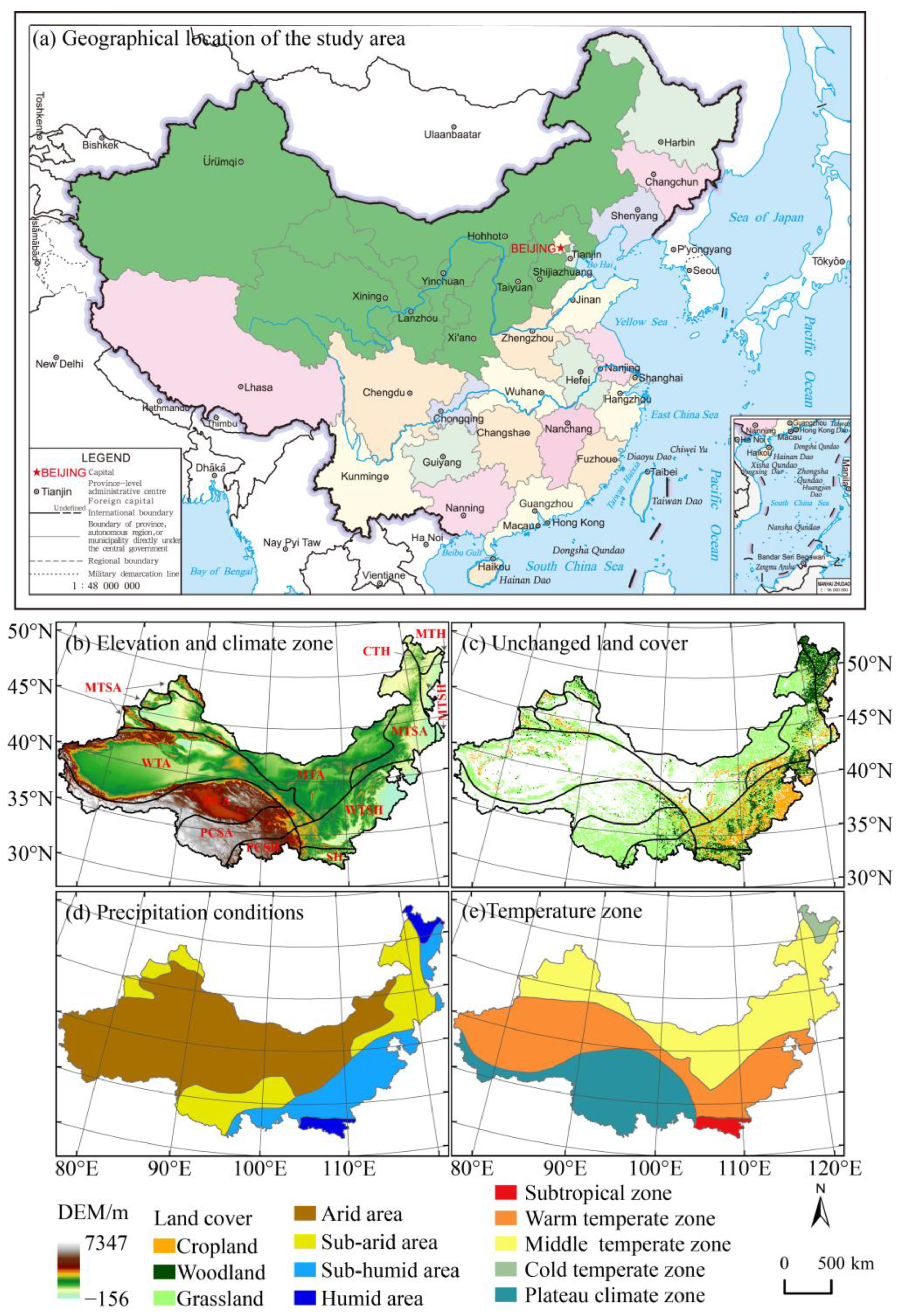
Figure 1. Geographical location of the study area (a); elevation and climate zone (b); unchanged land cover (c), precipitation conditions (d); and temperature zone (e) in the study area.
Remotesensing 14 06163 g001
Figure 2. Four different types of NDVI EEMD trends.
Remotesensing 14 06163 g002
Figure 3. Flow chart of the NDVI analysis methods and processes in the study area.
Remotesensing 14 06163 g003
Figure 4. Interannual variation trend of mean GSN of the study area and three different vegetation cover types. The red and blue lines indicate the linear and nonlinear trends, respectively.
Remotesensing 14 06163 g004
Figure 5. Spatial distribution of NDVI liner trend (a) and its significance (c), the average EEMD trend (b) and its significance (d) in growing season (Non-sig: Non-significant, G to B: Greening to browning, B to G: Browning to greening, G to G: Monotonic greening, B to B: Monotonic browning).
Remotesensing 14 06163 g005
Figure 6. The average trend for EEMD before (a) and after (b) the turning point (p < 0.05).
Remotesensing 14 06163 g006
Figure 7. Before and after the turning point, the significance of PCC between NDVI and temperature (a,b), precipitation (c,d) and solar radiation (e,f) and the spatial distribution pattern of climate control factor (g,h) in the growing season. Tem, Pre, SR represent temperature, precipitation, and solar radiation, respectively.
Remotesensing 14 06163 g007
Figure 8. The significance of PCC between NDVI with monotonic trend and non-significant trend and temperature (a,b), precipitation (c,d) and solar radiation (e,f) and the spatial distribution pattern of climate control factor (g,h) in the growing season. Tem, Pre, SR represent temperature, precipitation, and solar radiation, respectively.
Remotesensing 14 06163 g008
Figure 9. The relative contribution of climate change (a) and human activities (b) to vegetation change, and the spatial distribution of driving forces of vegetation dynamics (c). (ICH: NDVI increase caused by climate change and human activity; IHA: NDVI increase caused by human activity; ICC: NDVI increase caused by climate change; DCH: NDVI decrease caused by climate change and human activity; DCC: NDVI decrease caused by climate change; DHA: NDVI decrease caused by human activity).
Remotesensing 14 06163 g009
Table 1. Detailed information on 11 climate zones in the study area.
CodeClimate ConditionCodeClimate Condition
CTHCold-temperate humid zoneWTAWarm temperate arid zone
MTHMiddle temperate humid zonePCSHPlateau climate sub-humid zone
MTSHMiddle temperate sub-humid zonePCSAPlateau climate sub-arid zone
MTSAMiddle temperate sub-arid zonePCAPlateau climate arid zone
MTAMiddle temperate arid zoneSHSubtropical humid zone
WTSHWarm temperate sub-humid zone
Table 2. Assess the relative contribution of climate change (CC) and human activity (HA) drivers in vegetation dynamics under six scenarios.
SNDVISCCSHARelative Contribution
of CC
Relative Contribution
of HA
Driving Forces of Vegetation Dynamics
+++ | S C C | | S C C | + | S H A | | S H A | | S C C | + | S H A | Both CC and HA induced NDVI increase (ICH)
+1000CC induced NDVI increase (ICC)
+0100HA induced NDVI increase (IHA)
| S C C | | S C C | + | S H A | | S H A | | S C C | + | S H A | Both CC and HA induced NDVI decrease (DCH)
+1000CC and induced NDVI decrease (DCC)
+0100HA induced NDVI decrease (DHA)
Abbreviations: SNDVI, SCC and SHA represent the slopes of NDVI, NDVIc and NDVIh, respectively.
Table 3. Superposition statistics of linear and nonlinear trend type results (%).
Trend TypesNonlinear Trend Base on EEMD
Non-SigG to BB to GG to GB to BTotal
Mann-Kendall resultB to B2.022.650.1900.905.76
Non-sig30.709.364.501.770.2246.55
G to G7.234.1615.7820.52047.69
Total39.9516.1720.4722.291.12100
Abbreviations: Non-sig: Non-significant, G to B: Greening to browning, B to G: Browning to greening, G to G: Monotonic greening, B to B: Monotonic browning.
Table 4. The trend of vegetation GSN in different land cover types for EEMD (%).
Land Cover TypesNonlinear Trend Base on EEMD
Non-SigG to BB to GG to GB to BTotal
Cropland24.1318.2822.7733.900.92100
Woodland42.4420.6312.6123.061.26100
Grassland43.8014.4821.7418.841.14100
Abbreviations: Non-sig: Non-significant, G to B: Greening to browning, B to G: Browning to greening, G to G: Monotonic greening, B to B: Monotonic browning.
Table 5. Area percentage of vegetation controlled by different climate factors in different land cover types (%).
Land CoverBefore the Turning Point After the Turning PointMonotonic TrendNon-Significant Trend
TemPreSRTemPreSRTemPreSRTemPreSR
Cropland38.5735.3826.0525.0048.4126.5945.7639.0215.2220.6857.9721.35
Woodland41.4923.6334.8825.2738.3936.3436.1222.8441.0423.7728.0448.19
Grassland39.1137.0923.828.7443.4027.8652.7133.9013.3925.9555.1518.90
ALL39.3434.7825.8827.4743.7028.8348.0433.4718.4924.9950.8524.16
Abbreviations: Tem, Pre, SR represent temperature, precipitation, and solar radiation, respectively.
Table 6. The contribution rate of climate change (CC) and human activities (HA) to different types of vegetation dynamics in the study area from 1982 to 2015 (%).
TypesCroplandWoodlandGrasslandALL Land Cover
CCHACCHACCHACCHA
Vegetation restoration 37.1062.9057.6242.3854.3145.6951.2248.78
Vegetation degradation56.8043.2033.2366.7749.7250.2847.4352.57
Overall study area39.7360.2751.0448.9653.1446.8650.3349.67
Publisher’s Note: MDPI stays neutral with regard to jurisdictional claims in published maps and institutional affiliations.