Abstract
Optical remote-sensing images have a wide range of applications, but they are often obscured by clouds, which affects subsequent analysis. Therefore, cloud removal becomes a necessary preprocessing step. In this paper, a novel and superior transformer-based network is proposed, named Cloudformer. The proposed method novelly combines the advantages of convolution and a self-attention mechanism: it uses convolution layers to extract simple features over a small range in the shallow layer, and exerts the advantage of a self-attention mechanism in extracting correlation in a large range in the deep layer. This method also introduces Locally-enhanced Positional Encoding (LePE) to flexibly generate suitable positional encodings for different inputs and to utilize local information to enhance encoding capabilities. Exhaustive experiments on public datasets demonstrate the superior ability of the method to remove both thin and thick clouds, and the effectiveness of the proposed modules is validated by ablation studies.
1. Introduction
Remote-sensing imaging has a wide range of applications in various fields, such as identifying building areas [1], detecting environmental changes [2] and military reconnaissance. Since about 55% of land surface is covered by clouds [3], light is easily reflected and absorbed, compromising the quality of remote-sensing images. Specifically, cloud cover degrades remote-sensing image resolution and contrast, hindering downstream tasks such as target detection, semantic segmentation and so on. Therefore, cloud removal is an important preprocessing step in remote-sensing image analysis and interpretation. In recent years, researchers have carried out a wealth of research on the problem of cloud removal and have proposed various methods.
However, most of the current cloud-removal methods use traditional methods or convolutional neural networks. Traditional methods usually rely on artificially proposed prior assumptions and simplified physical models, which limit the generalization ability of the network. Although a deep convolutional network improves the generalization ability of the network through a data-driven approach, the convolution operation only focuses on a small part, and its weight usually remains fixed after the training is completed, which reduces the flexibility of the network and limits its ability to restore images.
Recently, the transformer structure has shown excellent performance in the field of computer vision [4,5,6,7,8,9,10]. It also has great potential to outperform existing mainstream approaches in the field of cloud removal. Compared to convolution, the self-attention mechanism [11] in a transformer has a larger receptive field and is able to compute dependencies over a larger range. This helps in areas obscured by clouds to recover ground feature information with reference to surrounding areas. In addition, unlike convolution with fixed weights after training, the self-attention mechanism can dynamically calculate weights according to different inputs. This is beneficial to enhance the flexibility of the network so that it can adapt to complex and diverse remote-sensing image scenes.
Although the transformer structure has many advantages, due to relaxation of the constraints on the network, it usually requires large-scale datasets for training to avoid overfitting. However, it is not easy to collect large-scale cloud-removal datasets, which inspires us to combine transformers and convolutions to improve the cloud-removal ability of the network. At present, there is the lack of a method that can combine well the characteristics of a self-attention mechanism and convolution. In order to solve the above problem, we propose a transformer-based cloud-removal network combining convolution and a self-attention mechanism, named Cloudformer. The main contributions of our proposed method are as follows:
- We use the convolution layers to replace the self-attention mechanism in the shallow layer of the network to extract simple features over a small range. Window-based Multi-head Self-Attention (W-MSA) is used in the deep layers of the network to calculate dependencies on a larger scale. Thus, convolution and self-attention are combined well to improve network performance.
- A transformer-based U-shaped encoder–decoder residual symmetric network architecture is used to achieve end-to-end cloud removal, enhancing the network’s ability to remove thin and thick clouds.
- Locally-enhanced Positional Encoding (LePE) [12] is introduced into W-MSA. Different from the commonly used relative position encoding that remains fixed for different inputs after training, LePE is based on depthwise convolution, which can generate different position encodings for different inputs.
- Comparative experiments on the thin-cloud dataset RICE1, the thick-cloud dataset RICE2 and the synthetic-cloud Paris dataset demonstrate that our method outperforms the other four methods, and the effectiveness of the proposed method is verified by experiments and visual analysis.
The rest of this article is structured as follows. In Section 2, we introduce related work, including cloud-removal methods and vision transformers. Section 3 elaborates on our proposed method. Section 4 shows the experimental results, verifying the effectiveness of modules by ablation studies and the superiority of the method by comparing it with four other methods. Conclusions are drawn in Section 5.
2. Related Works
2.1. Cloud Removal Methods
Generally speaking, cloud-removal methods are divided into thin-cloud removal and thick-cloud removal according to cloud layer thickness. In terms of thick clouds, since the ground objects are completely obscured by clouds, it is difficult to infer the surface information from just one picture. The common approach is to introduce auxiliary information to help remove thick clouds. Unlike thick clouds, some light can pass through thin clouds, so some surface information is preserved in remote-sensing images, and cloud removal is more likely to be achieved with only a single image.
2.1.1. Thick-Cloud Removal Methods
First, we introduce thick-cloud-removal methods, which can be divided into multi-temporal methods and multi-source methods. Multi-temporal methods remove clouds by introducing remote-sensing images taken at different times. This is because the position of clouds changes over time: an area obscured by clouds at one time may be cloud-free at another time, so the information can complement each other. Lin et al. [13] proposed a method to clone cloud-free patches onto cloud-obscured patches by solving the Poisson equation. Cheng et al. [14] proposed a method based on Markov random fields to find suitable pixels for replacing cloud-contaminated ones. Li et al. [15] extended two dictionary-learning algorithms to better implement multitemporal cloud removal. Chen et al. [16] proposed an innovative spatially and temporally weighted regression model to better utilize complementary information. Based on robust principal component analysis (RPCA), Wen et al. [17] developed a method that includes a plain RPCA for cloud detection and a discriminative RPCA for image reconstruction. Unlike most methods that require cloud masks or separate cloud detection, Ji et al. [18] propose a method for simultaneous cloud detection and cloud removal. A possible problem is that the ground objects can change drastically at different times, which most multi-temporal methods cannot handle well.
Another approach is multi-source methods [19,20,21,22], which bring in data from different sensors as an aid. Based on the Closest Spectral Fit (CSF) [23] method, Eckardt et al. [19] proposed a method for assisted removal of thick clouds from multi-spectral images using synthetic aperture radar (SAR) data. Li et al. [22] proposed a convolutional neural network capable of recovering information from high-resolution images with reference to SAR images and low-resolution optical images.
Although the above methods have achieved good results, they still have some inherent defects. For multi-temporal methods, a possible problem is that the ground objects can change drastically at different times, affecting the correctness of the results. Further, for multi-source methods, it is difficult to fuse images of different resolutions and imaging mechanisms well without generating false information.
2.1.2. Thin-Cloud Removal Methods
As for thin-cloud-removal methods, they can be divided into traditional methods and deep learning methods. In terms of traditional methods, a classic method based on dark-object subtraction was proposed by Chavez et al. [24]. Taking advantage of the fact that the spectral responses of different objects are highly correlated under cloud-free conditions, and that this correlation is destroyed by clouds, haze optimized transformation (HOT) [25] has been proposed. An improved version was proposed by He et al. [26]. Since clouds tend to correspond to low-frequency components in the image, wavelet analysis [27] and homomorphic filtering [28,29] have been effectively applied. Using the cirrus bands of Lansat 8 OLI, Xu et al. [30] proposed a method based on linear regression. Xu et al. [31] proposed a method based on a physical model that considers both reflection and absorption of radiation. In addition, some methods for dehazing of visual images can also be applied in the field of cloud removal. The dark channel prior [32] is a classical method that works by assuming that there are a few pixels in the local area of the haze-free image of the outdoor environment that have very low values on at least one channel.
In general, traditional methods are often based on some signal-processing techniques and prior knowledge, requiring specialized knowledge to select the appropriate one. Further, it is difficult for these methods to take into account complex and changeable situations, resulting in poor generalization performance.
Deep convolutional networks have achieved excellent results in the field of cloud removal due to their good generalization performance and strong fitting ability. Without the need to provide a lot of prior knowledge or simplifying assumptions, deep convolutional networks can automatically learn complex mapping relationships directly from large amounts of data. Li et al. [33] designed an encoder–decoder network based on residual connections for end-to-end cloud removal. Wang et al. [34] applied a conditional Generative Adversarial Network (cGAN) [35] to images occluded by thin and thick clouds. Enomoto et al. [36] proposed the Multispectral conditional Generative Adversarial Network (McGAN) by generalizing cGAN to images containing visible and near-infrared bands. An attention mechanism has been introduced to better handle the problem of uneven spatial distribution of clouds [37,38], and the network pays more attention to areas with thicker clouds. Typically, deep learning methods require pairs of images, including cloudy and cloudless images of the same location. However, it costs a lot to collect paired images. Further, due to the different sampling times of cloudy images and cloudless images, the ground object information may change, which makes the collection of datasets more difficult. Some approaches attempt to reduce the cost of data collection by relaxing dataset requirements. By using a combination of adversarial loss and cycle consistency loss [39], Singh et al. [40] proposed Cloud-GAN, which can be trained without using paired datasets. Combining generative adversarial networks and physical models, Li et al. [41] proposed a semi-supervised method: CR-GAN-PM.
However, convolutional networks have some inherent deficiencies. First of all, since the convolution operation only has a small receptive field, it is difficult to restore the cloudy area in a large range with the help of a far area. Secondly, the weights of convolution kernels remain fixed during prediction and cannot be flexibly changed according to different inputs. To alleviate these problems, some methods [42,43] have introduced the transformer structure for thin- and thick-cloud removal. However, since the self-attention mechanism lacks the inductive bias similar to convolution, simply using the transformer structure can easily cause overfitting and lead to a decline in generalization ability, in the absence of large-scale datasets. It is necessary to cleverly combine self-attention and convolution to better adapt to remote-sensing image cloud-removal tasks.
2.2. Vision Transformers
The Vision Transformer (ViT) [4] has achieved state-of-the-art results on image classification tasks, indicating that the transformer has begun to challenge the dominance of convolutional neural networks (CNNs) in the image field. Several methods have been developed for other vision tasks, such as low-level tasks [5,6], object detection [7,8] and semantic segmentation [9,10].
A transformer module consists of a Multi-Head Self-Attention module (MHSA) and a Feed-forward module (FFN). The Self-Attention module [11] can calculate long-range correlation and can dynamically determine the attention weight according to the input, which is different from the convolutional module, which only focuses on local parts and maintains static weights. Some works have tried to combine transformers and convolutions to take advantage of their respective advantages. CvT [44] uses convolution to replace linear projection in a self-attention mechanism to better capture local information. The authors of [45,46] add depth-wise convolution to the Feed-forward module to enhance the locality of the transformer network. Uniformer [47] uses convolution to model local information in the shallow layers and self-attention in the deep layers to capture long-range correlations, making the network more efficient.
Since the self-attention mechanism needs to calculate the correlation globally, the complexity of the calculation is the quadratic of the image size, which brings an excessive amount of calculation to tasks that use large-size images. Many methods [48,49,50] have chosen to introduce window attention, using self-attention within a local window instead of computing it globally, thus greatly reducing computational overhead. These methods usually require some means to promote the information interaction between windows, such as shifting [50], shuffling [48] and/or the haloing operation [51].
Unlike convolution, which introduces local inductive bias, the self-attention mechanism does not introduce positional information when calculating the correlation. Thus, it is often necessary to add positional encoding to make up for this defect. Generally speaking, position encoding methods can be divided into absolute position encoding (APE), relative position encoding (RPE) and convolution-based position encoding. APE usually adds the positional encoding that can be obtained by the sinusoidal functions [11] or by learning [52] to the inputs. Different from APE, RPE [50,53,54,55,56] abandons the focus on absolute positions and instead focuses on the relative position information of input tokens. APE and RPE both have some deficiencies. First, these two methods usually generate fixed position encodings for different inputs during prediction, thus lacking flexibility. Second, they do not bring in surrounding information to aid in encoding. Convolution-based position encoding [12,57] exploits the locality of convolution to introduce position information. Due to the characteristics of convolution, it cannot only generate different positional encodings depending on the inputs but can also enhance network performance with local information.
Although the transformer has excellent performance in the image field, it often requires a larger dataset for training because it relaxes the constraints on the network. However, for the field of remote-sensing image cloud removal, it is not easy to obtain a large number of training samples. Due to the existence of cloud cover, we cannot obtain cloud-contaminated and cloudless images of the same area at the same time. Additionally, images taken at different times may not completely correspond due to changes in ground objects and lighting. Therefore, collecting large cloud-removal datasets is not an easy task, which limits the application of transformers. It is necessary to combine a transformer and convolution to design a network structure that is more suitable for cloud removal.
3. Method
In this section, we first introduce the overall architecture of Cloudformer and the pipeline. Then, we describe the structure of the Cloudformer block in detail, including the Convolution Cloudformer block (CCB) and the Self-Attention Cloudformer block (SACB), and explain the design ideas based on visualization.
3.1. Architecture of Cloudformer
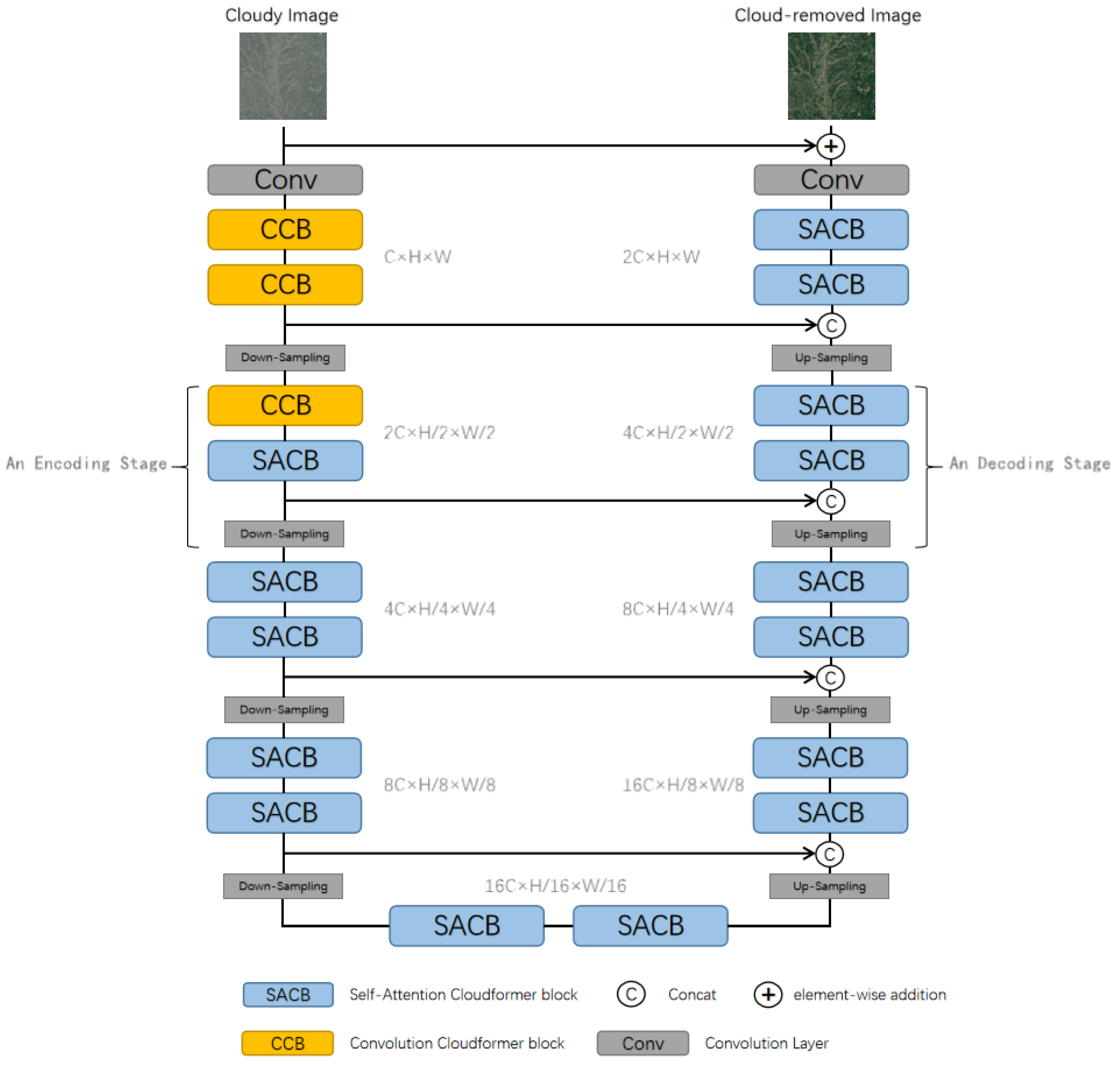
The structure of Cloudformer is designed on the basis of Uformer [58]. Innovatively, we replace the self-attention in the shallow layers of Uformer with the convolutional layers and introduce Locally-enhanced Positional Encoding (LePE) into the Window-based Multi-head Self-Attention (W-MSA). As Figure 1 shows, Cloudformer is a U-shaped transformer-based encoder–decoder structure network that uses skip connections to pass information between different stages. A cloudy image is taken as the input of the network, and the output is a cloud-removed image .
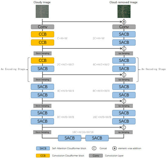
Figure 1.
Overall architecture of Cloudformer.
Specifically, the input image first goes through a convolutional layer, which keeps the height and width of the image unchanged and increases the number of channels to , which is equal to 16 in our settings. The feature map is then fed into a series of Cloudformer blocks and downsampling layers for encoding. The Cloudformer block is used to extract image features without changing the size of the feature map, and the downsampling layer is a convolution with a stride of 2, which halves the height and width of the feature map and doubles the number of channels. The network contains a total of four stages of encoding, each stage contains two Cloudformer blocks and a downsampling layer. Since the network mainly extracts simple features in the neighborhood in the shallow layer, we use the Convolution Cloudformer block (CCB) in these layers, which uses convolution layers instead of the self-attention mechanism to avoid redundant computation and overfitting. In the deep layer, we use the Self-Attention Cloudformer block (SACB) based on Window-based Multi-head Self-Attention (W-MSA) to calculate the correlation in a larger range and to extract more complex features. Specifically, the first three Cloudformer blocks are CCB, while the others are SACB.
After four encoding stages, the feature map needs to go through a bottleneck that consists of two SACBs. After this, the network enters the decoding phase, which is accompanied by an increase in the size of the feature map and a decrease in the number of channels. Corresponding to the encoding stage, there are four decoding stages, each containing an upsampling layer and two SACBs. The upsampling layer is a convolution with a stride of 2, so as to double the height and width of feature maps. After each upsampling layer, we concatenate the feature maps in the channel dimension with feature maps of corresponding dimensions in the encoding stages, which can improve the information exchange between upstream and downstream. The concatenated feature maps are input into SACBs to calculate the correlation between a larger range and to restore the image information.
After completing the decoding stage, the feature map is input into a convolutional layer, and then it is added element-by-element to the input to get the final output image .
As for the loss function, we follow the previous study to use Charbonnier loss [58,59,60], which is a variant of the L1 loss. The loss function expression is as follows:
where represents the ground-truth cloud-free image, and is a small constant, which is set to .
3.2. Cloudformer Block
Unlike CNNs, which only focus on local information, thanks to the self-attention mechanism, a transformer can calculate dependencies on a larger range, which is considered an important reason why it can surpass CNNs. However, according to previous research [47], vision transformers tend to extract local information in the shallow layer, while extracting information in a larger range in the deep layer. This phenomenon means that using self-attention at shallow layers is not efficient because computing a larger range of dependencies actually results in redundant computation. Considering that large-scale remote-sensing image cloud-removal datasets are not easy to obtain, it is necessary to reduce redundant computation and parameters to prevent the network from overfitting on small- and medium-sized datasets.
In order to elucidate the above phenomenon more clearly and to verify whether it holds on the cloudless network, we take out the self-attention weights of the shallow and deep layers of the network and analyze them visually. We replace the convolution layers in CCB back to the original Window-based Multi-head Self-Attention (W-MSA) and use relative position encodings in all Cloudformer blocks. Then, we output the self-attention weights for the 1st and 10th blocks in the network, average the values across all windows, and visualize them in Figure 2. It is worth pointing out that since W-MSA only calculates correlations between tokens within a window, the corresponding self-attention heatmap size is , where M corresponds to the size of the window: . We enlarge the heatmap to the same size as the input image just for convenience.
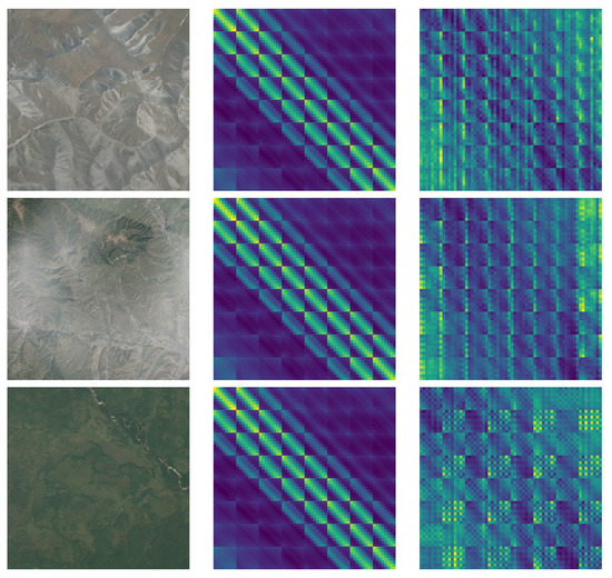
Figure 2.
Visualization of self-attention weights for the 1st and 10th blocks in the network. The first column represents the input cloud-contaminated image. The second column represents the heatmaps corresponding to the average self-attention weight of all windows in the 1st block. The third column represents the heatmaps corresponding to the average self-attention weight of all windows in the 10th block. It can be seen from the figure that the heatmaps present a diagonal distribution in the shallow layer of the network, which indicates that the self-attention weight is mainly generated in the neighborhood of tokens. In contrast, in the deeper layers of the network, the heatmaps are uniformly distributed, which indicates that the self-attention mechanism is effective in the entire window.
It can be clearly seen in Figure 2 that in the shallow layer of the network, the heatmaps present a diagonal distribution, which indicates that the self-attention weight is mainly generated in the neighborhood of tokens. Further, for different input images, the shallow self-attention weight distribution does not change much. In contrast, in the deeper layers of the network, the heatmaps are uniformly distributed, which indicates that the self-attention mechanism is effective in the entire window. Based on the above analysis, we propose to use CCB in the shallow layers and SACB in the deep layers to reduce redundant computation and to improve the network performance.
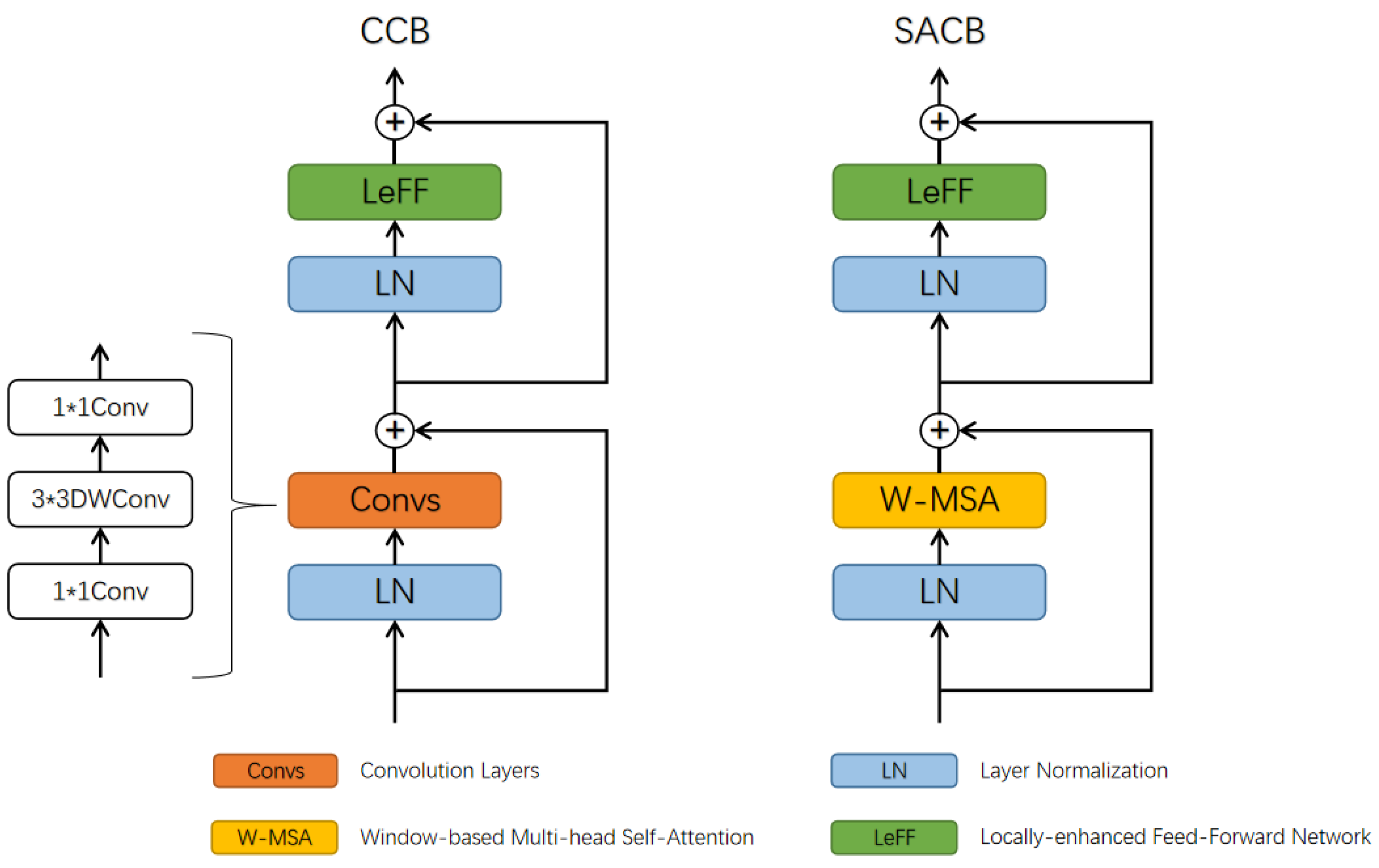
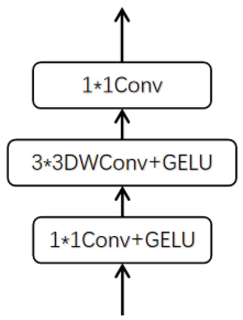
As shown in Figure 3, CCB and SACB share a similar structure: the difference is that CCB replaces the W-MSA in SACB with convolution layers, which contain two convolutions and one depthwise convolution, to extract simple features in a smaller neighborhood and to avoid redundant computation. For these two modules, the features are first subjected to layer normalization, and then a feature-extraction module is used to capture the dependencies between tokens, corresponding to convolution layers and W-MSA in CCB and SACB, respectively. Then, after a skip connection, the features are again subjected to layer normalization and input to the Locally-enhanced Feed-Forward Network (LeFF) [45,46], which is composed of three layers of convolution. As shown in Figure 4, unlike the usual Feed-Forward Network in a transformer, LeFF adds a depthwise convolution in the middle that can utilize local information to enhance the modeling ability of the network. Finally, the results are obtained through the second skip connection after LeFF.
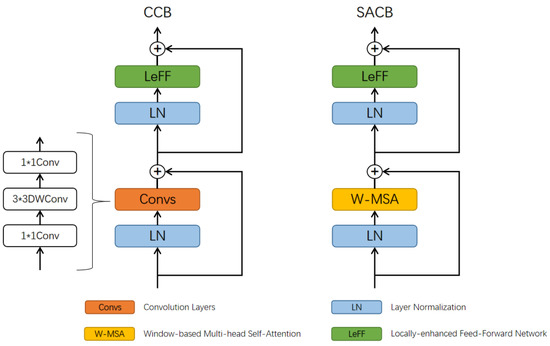
Figure 3.
Structure of Convolution Cloudformer block (CCB) and Self-Attention Cloudformer block (SACB).
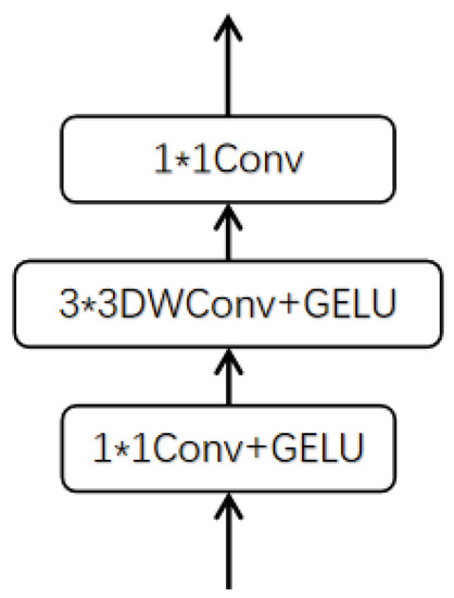
Figure 4.
Structure of LeFF.
3.2.1. Self-Attention Cloudformer Block (SACB)
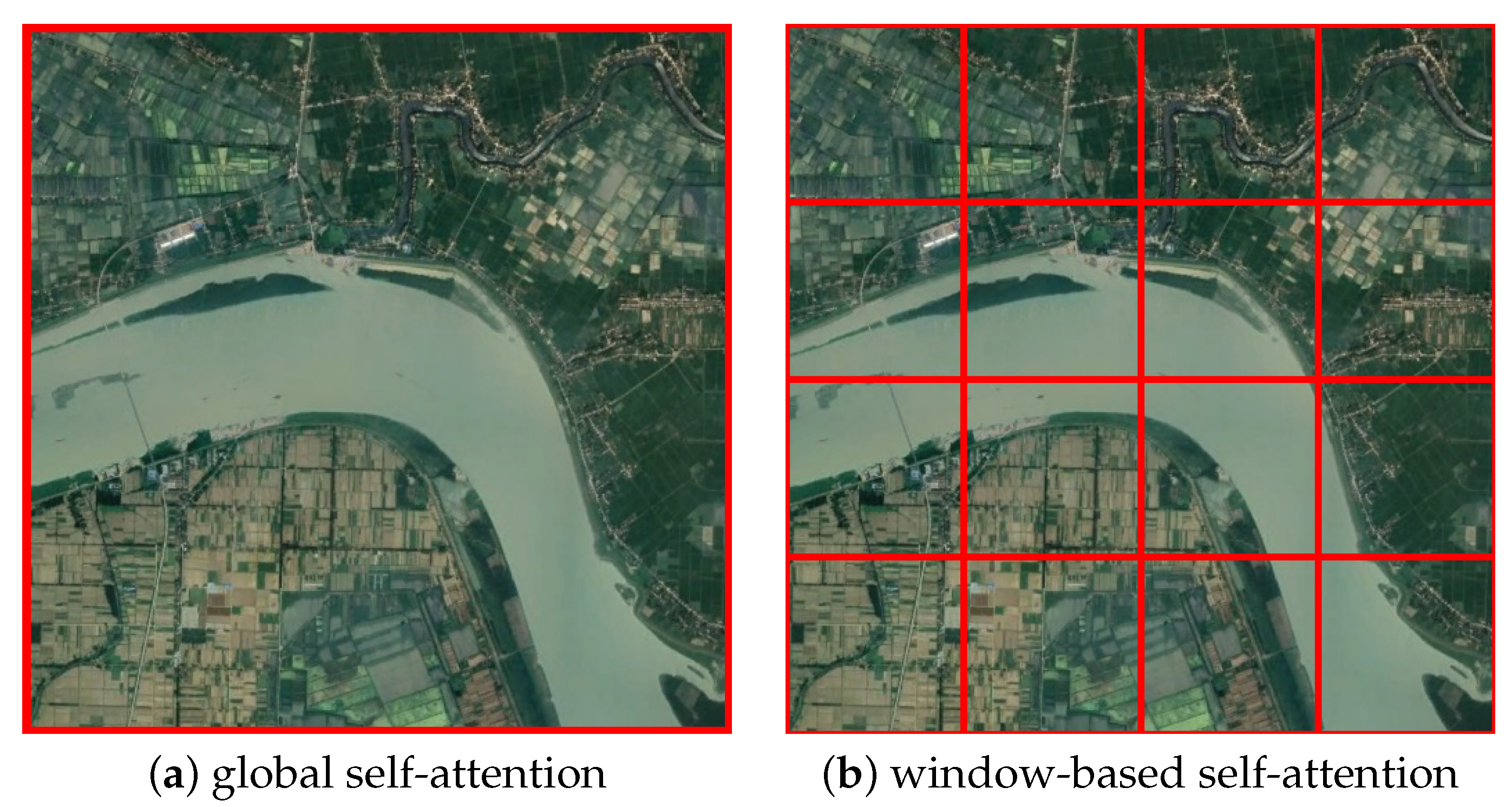
Window-based Multi-head Self-Attention (W-MSA): Instead of using the global self-attention in the original transformer, whose computational complexity is a quadratic of the image size, we choose window-based self-attention [50], which implements self-attention only within the window, as Figure 5 shows, to reduce the computational complexity to be linear with respect to the image size.
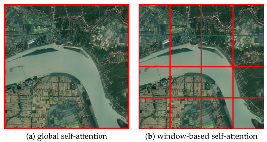
Figure 5.
Global self-attention computes dependencies across the entire feature map. Window-based self-attention only calculates dependencies within the window range, so it can reduce the amount of calculations.
Specifically, for the input feature map , we divide it into N windows of size in the spatial dimension, as shown in Figure 5b, and implement multi-head self-attention within the window. The calculation process is as follows:
represents splitting the feature map in the spatial dimension and reshaping small pieces of feature maps to -sized tokens. are used to linearly transform these tokens, where k represents the corresponding k-th head. In the actual setting, we adjust the number of heads so that is equal to C. After the self-attention mechanism, we concatenate in the head dimension and perform a linear transformation through to get . Finally, they are combined and restored to their size prior to through .
Locally-enhanced Positional Encoding (LePE): Window-based Self-Attention often uses relative position encoding [50,53],
where is the position bias generated according to the relative positional relationship between tokens. Since there are cases for the relative position of each dimension, there are cases for the relative position in the two-dimensional space. Thus, B can be generated from trainable parameters.
However, after the training is completed, does not change for different inputs and lacks the utilization of local information. Therefore, we adopt Locally-enhanced Window-based Self-attention by introducing Locally-enhanced Positional Encoding (LePE) into W-MSA [12],
where is obtained by reshaping . means depthwise convolution, and the size of the convolution kernel is by default.
For different inputs , this method can generate suitable positional encodings through depthwise convolution. Further, due to the local receptive field of convolution, local information can be introduced into position encodings to enhance the network performance.
3.2.2. Convolution Cloudformer Block (CCB)
Based on the previous analysis, two assumptions can be made: first, the self-attention mechanism only produces significant weights in the neighborhood of tokens in shallow layers; and second, the distribution of self-attention weights in shallow layers does not vary with changes to the input cloudy image. These two assumptions can be expressed mathematically as follows:
where represents the self-attention weight between i-th and j-th tokens on the k-th head. represents the i-th and j-th token, respectively. represents the relative position between and on the feature map. represents a space of size around on the feature map. If does not belong to , the corresponding self-attention weight is zero.
Under the above assumptions, if the number of heads is equal to the number of channels of tokens, the self-attention mechanism will degenerate into a series of convolutions. Specifically, for the input feature map , we flatten it in the spatial dimension to get and then feed it into the self-attention mechanism:
where represents the ordinary convolution, and represents the depthwise convolution. In practice, k is set equal to 3. It can be seen from the above derivation that the first corresponds to the generation of value . corresponds to the multiplication of the self-attention weight and , and the second corresponds to the use of for linear transformation. Based on the above assumptions and analysis, we choose to use convolutions to replace W-MSA in SACB to obtain CCB so as to reduce redundant computation, prevent overfitting, and improve network performance.
4. Experimental Results
4.1. Description of Dataset
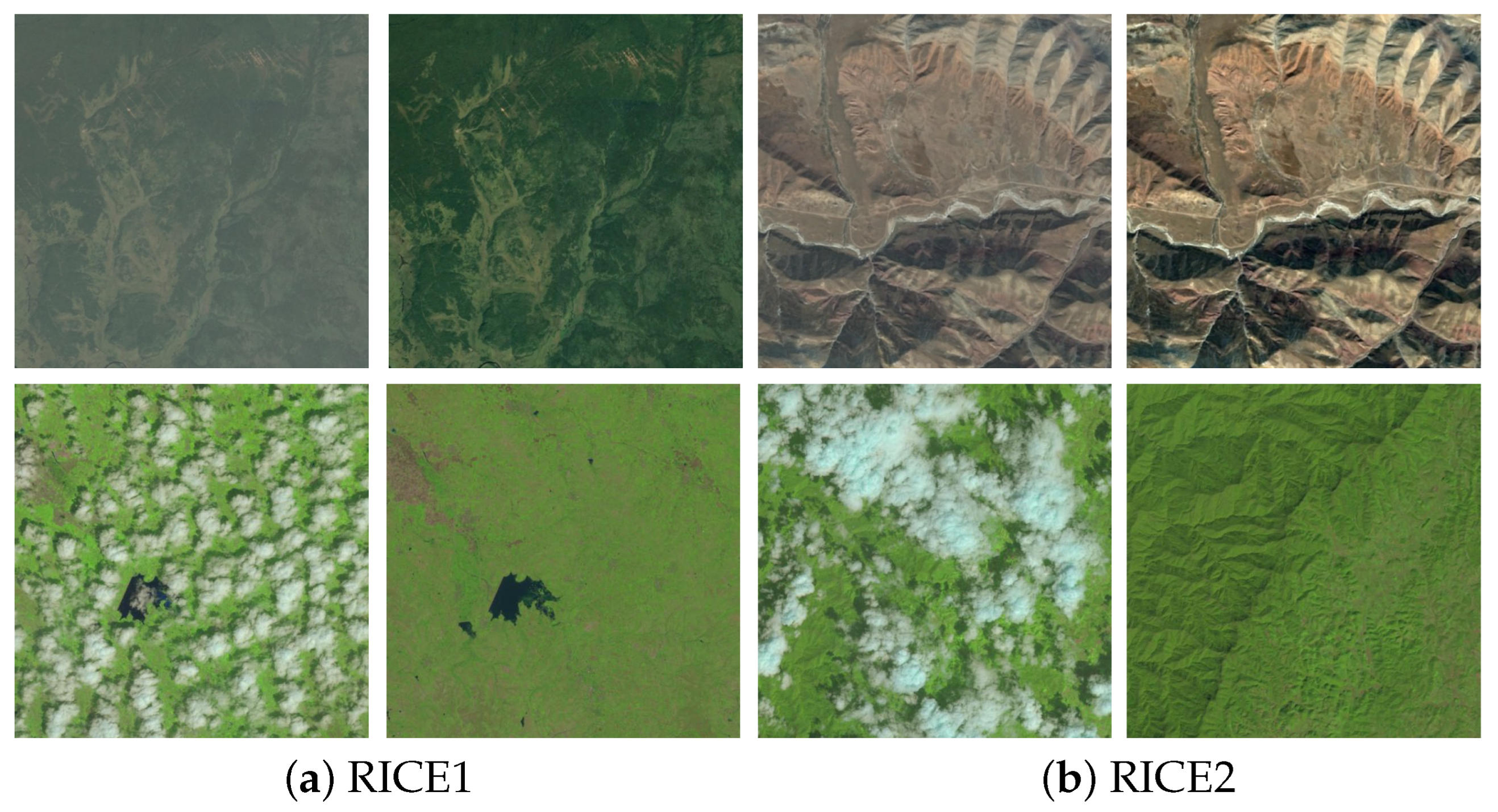
We conduct experiments on a publicly available optical remote-sensing dataset named RICE [61]. The RICE dataset consists of two parts: thin-cloud dataset RICE1 and thick-cloud dataset RICE2. RICE1, obtained from Google Earth, has 500 pairs of images, each of which contains one image with thin cloud(s) and one image without clouds. The thick-cloud dataset, RICE2, is obtained from Landsat 8 OLI/TIRS and has 736 pairs of images with a time interval of no more than 15 days. The image size in both RICE1 and RICE2 is . Typical samples of RICE1 and RICE2 are shown in Figure 6.

Figure 6.
A typical sample presentation of the RICE dataset: (a) RICE1 dataset—images with thin cloud are on the left and without cloud are on the right. (b) RICE2 dataset—images with thick clouds are on the left and without clouds are on the right.
We divide each dataset into three parts for training, validation and testing, at a ratio of 64%, 16% and 20%, respectively. Therefore, the number of training set, validation set and test set samples in RICE1 is 320, 80 and 100, respectively. The number of training set, validation set and test set samples in RICE2 is 470, 118, 148, respectively. We select the model parameters with the highest PSNR on the validation set for testing.
4.2. Training Details and Evaluation Metrics
We use the PyTorch framework to implement Cloudformer and use two RTX 3090 GPUs for training. The AdamW [62] algorithm is used to optimize the parameters, and the initial learning rate is set to 0.0002. The momentum terms are set to (0.9,0.999), and the weight decay is equal to 0.02. We set the batch size to 2 and the epoch to 750.
We use the general evaluation indicators of peak signal-to-noise ratio (PSNR) and structural similarity index measurement (SSIM) in the field to verify the performance of the algorithm. Given two images x and X, PSNR and SSIM are calculated as follows:
where is the maximum value that a pixel can take. The higher the values of PSNR and SSIM, the closer the recovered image is to ground-truth. The symbols () and () represent the mean and variance of the corresponding image, respectively; represents the covariance between x and X; and and are constants used to maintain stability. For multi-channel images, SSIM is obtained by first calculating separately on each channel and then averaging.
4.3. Network Architecture Analysis
We investigate the utility of modules in Cloudformer by controlling-variable experiments. In order to conduct experiments more conveniently, we design a “UNet” by replacing each Cloudformer block in our proposed network with a convolutional layer with a LeakyReLu activation function. Table 1 shows quantitative results on the RICE1 test set under different network architectures. Among them, Method 1 corresponds to the convolutional network “UNet”. Method 2 represents replacing all blocks in Cloudformer with SACB using relative positional encoding. Method 3 is obtained by replacing the first three blocks in Method 2 with CCB. On the basis of Method 3, Method 4 changes the positional encoding method of SACB from relative positional encoding (RPE) to LePE. In fact, Method 4 is Cloudformer.

Table 1.
PSNR and SSIM on RICE1 test set with different architectures.
4.3.1. Comparison of Transformer and CNN
By comparing Method 1 and Method 2 in Table 1, it is clear that replacing the convolution with SACB can effectively improve the quantitative indicators on the RICE1 test set, which verifies the effect of the transformer structure on the cloud-removal field. Compared to 34.128 dB (PSNR) and 0.975(SSIM) for Method 1, Method 2 improves PSNR by 0.669 dB and SSIM by 0.002 by converting to a transformer structure. This proves that the transformer structure can effectively improve the de-cloud capability of the network.
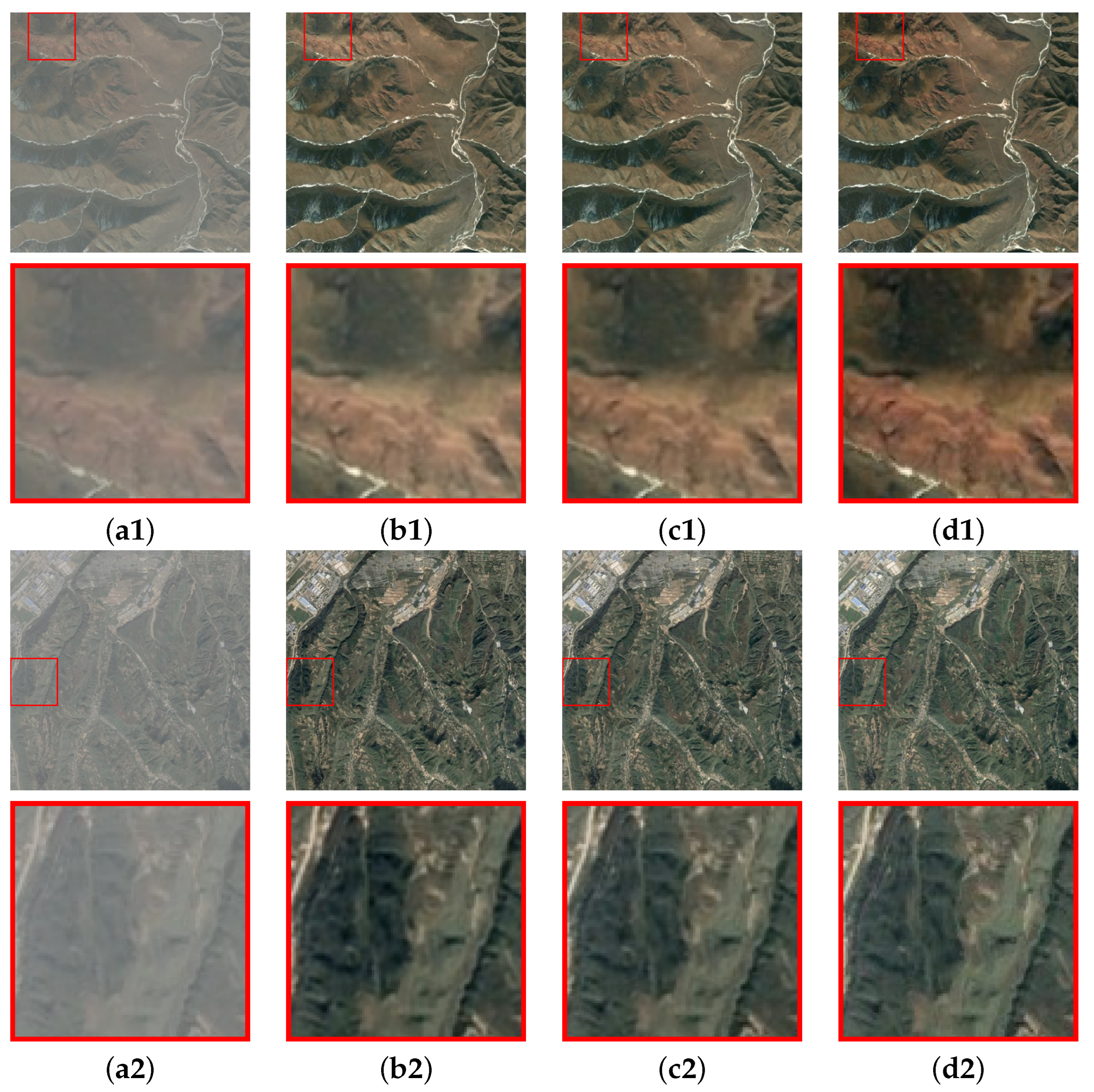
In order to more intuitively show the difference between the effect of the transformer structure and CNN, and to perform qualitative analysis, we show the results of two samples in the RICE1 test set in Figure 7. We marked the close-up area with a red box and placed it below the image for comparison. It can be clearly seen from Figure 7b1,c1 that the results of CNN have a large degree of color deviation, the overall color is light, and the contrast is poor. The image restored by the transformer structure has more vivid colors, stronger contrast, and is closer to ground-truth. By comparing b2 and c2 in Figure 7, it can be seen that there is a significant deviation in the brightness of the image recovered by the CNN structure. b2 is obviously too dark, causing some details in the image to be too dark to be displayed clearly. Further, c2 is brighter and closer to ground-truth. To sum up, the transformer structure shows better results than CNN in restoring the brightness and color of images. One possible reason is that the weights of the convolution kernel in CNN generally cannot change according to the change of the input, while the self-attention mechanism in the transformer can calculate different weights according to different inputs, so it has stronger fitting ability.
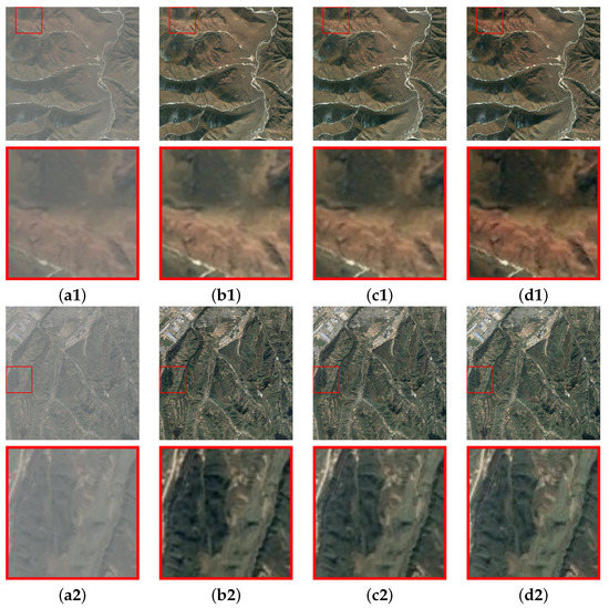
Figure 7.
Comparison of the effects of CNN and transformer structures on two RICE1 samples. (a1,a2) represent the input cloudy images. (b1,b2) represent the results of the CNN which corresponds to Method 1 in Table 1. (c1,c2) represent the results of the transformer which corresponds to Method 2 in Table 1. (d1,d2) represent the groudtruth images. The transformer structure shows better results than CNN in restoring the brightness and color of images.
4.3.2. The Trade-Off between Convolution and Self-Attention
As we can see in Table 1, by replacing the first three SACBs using relative position encoding in Method 2 with CCBs, in other words, by replacing the first three self-attention mechanisms with convolutions, the performance of the network is effectively improved. Specifically, from Method 2 to Method 3, PSNR increased by 0.24 dB and SSIM increased by 0.001. This verifies our previous idea that replacing the shallow self-attention mechanism of the network with convolution to extract simple features over a small range can prevent redundant calculations and parameters, thereby improving the cloud-removal performance of the network.
We also conduct experiments to investigate the optimal trade-off between SACB and CCB. To explore the number of CCBs that should be used, the top N blocks in Method 2 is replaced by CCBs, while the rest block use SACBs based on relative position encoding. The value of N ranges from 0 to 8. Quantitative analysis is performed on RICE1.
As shown in Figure 8, in general, when the number of CCBs increased from 0 to 3, the PSNR on the RICE1 test set showed an upward trend. As the number of CCBs increased from 0 to 3, the PSNR increased from 34.797 dB to 35.037 dB. However, as the number of CCBs exceeds 3, the PSNR shows a downward trend with the number of CCBs. It dropped from a peak of 35.037 dB to a minimum of 34.676 dB. This phenomenon is also in line with our previous analysis. Since the network mainly focuses on simple features over a small range in the shallow layer, the use of convolution-based CCB in the shallow layer is beneficial to improve the performance of the network. As a result, when the number of CCBs is small, it can usually bring positive promotion to the network. But when entering the deep layer, the network tends to extract complex features in a larger range, and continuing to use convolution at this time will limit the ability of the network and lead to performance degradation. Therefore, when the number of CCBs is too large, the PSNR generally tends to decrease with the increase of the number of CCBs. Since the PSNR value reaches the highest when the number of CCBs is 3, we specify the first 3 blocks as CCBs in Cloudformer.
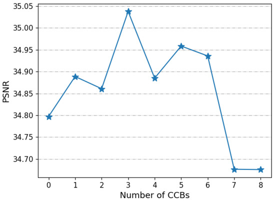
Figure 8.
PSNR vs. Number of CCBs. Test on RICE1.
4.3.3. Positional Encoding
Comparing Method 3 and Method 4 in Table 1, we can verify the effect of introducing Locally-enhanced Positional Encoding (LePE). By introducing LePE to replace RPE in SACB, the PSNR on RICE1 test set is improved by 0.206 dB. This verifies the effect of LePE, indicating that its adaptive determination of position encoding according to the input and the ability of using local information are helpful for the improvement of network performance.
4.3.4. Window Shift
For the window-based self-attention mechanism, previous studies have proposed various ways to promote the interaction between windows. We choose window shift [50] to determine whether a similar mechanism needs to be added to facilitate the interaction of information between windows. We add a window shift mechanism to each SACB in Cloudformer and compare it with the original results. The results are shown in Table 2. As we can see, the window-shift mechanism only improves PSNR by 0.004dB, which is almost indistinguishable. One possible reason is that removing clouds only needs to rely on a certain range of information, which can be obtained within one window, so the interaction between multiple windows is too redundant. Thus, we choose not to use window shift in Cloudformer in order to save cost.

Table 2.
Quantitative results of Cloudformer with and without window shift on the RICE1 test set.
4.4. Results on RICE1
We quantitatively compare the results of the proposed method on the RICE1 test set with four deep learning methods: Conditional GAN [35], McGAN [36], Spa GAN [37] and MSGAN [63]. As can be seen from Table 3, our method outperforms other methods on evaluation metrics. In terms of PSNR, our method achieves 35.243 dB, outperforming the second-best result of 32.170 dB by 3.073 dB. Further, in terms of SSIM, our method achieves 0.978, outperforming the second-best result of 0.965 by 0.013. The experimental results strongly demonstrate the superiority of our method.

Table 3.
Quantitative evaluation on RICE1.
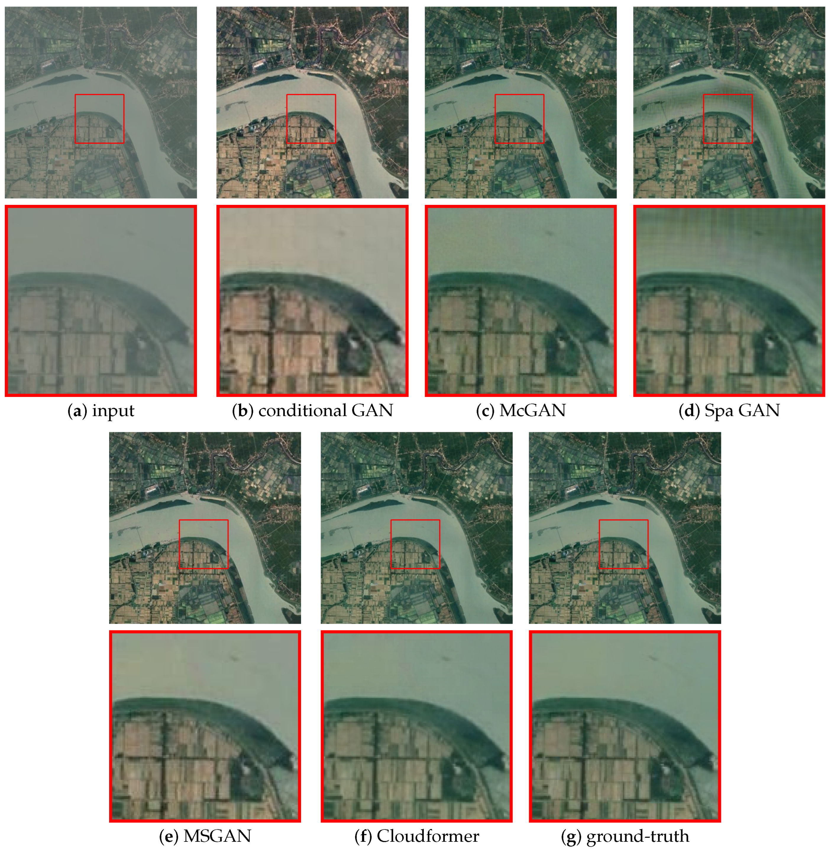
In order to show the effect of our method more intuitively, we show the cloud-removal effect of two samples in Figure 9 and Figure 10, respectively. As shown in Figure 9, the results of both conditional GAN and MSGAN show obvious color deviation, reflecting the limited fitting ability of the network. The results of Spa GAN show uneven brightness in river regions and wrong textures. In contrast, the color of the result of Cloudformer is closer to the ground-truth; there is no obvious wrong texture, and good smoothness maintained. In Figure 10, MSGAN produces obvious false patches in the upper left and right of the close-up, which may be caused by inappropriate sizes of convolution kernels. The results of McGAN and Spa GAN show a certain color deviation, which may be caused by insufficient network fitting ability. The texture features of the results of conditional GAN are relatively blurred and cannot reproduce image details well. In contrast, relying on the powerful fitting ability of the transformer structure, our results not only maintain the correctness of the color but also clearly preserve the texture characteristics of the image.
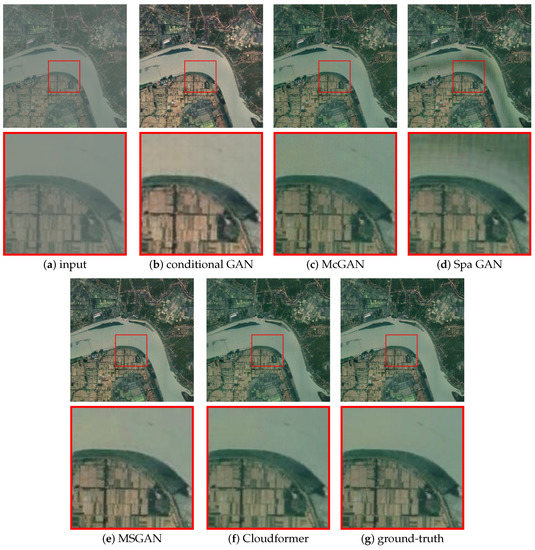
Figure 9.
Comparative experimental results on the first sample of RICE1. The results of both conditional GAN and MSGAN show obvious color deviation. The results of Spa GAN show uneven brightness in river regions and wrong textures. In contrast, the color Cloudformer’s result is closer to the ground-truth, there are no obvious wrong textures, and good smoothness is maintained.
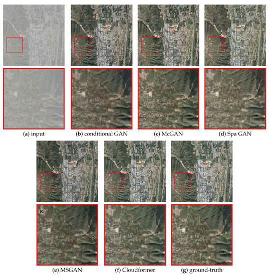
Figure 10.
Comparative experimental results on the second sample of RICE1. MSGAN produces obvious false patches in the upper left and right of the close-up. The results of McGAN and Spa GAN show a certain color deviation. The texture features of the results of conditional GAN are relatively blurred and cannot reproduce image details well. In contrast, our method not only maintains the correctness of the color but also clearly preserves the texture characteristics of the image.
4.5. Results on RICE2
Table 4 shows the quantitative comparison of Cloudformer and other methods on the RICE2 test set. Our proposed method also shows excellent performance in thick-cloud removal, surpassing other methods in evaluation indicators. The PSNR of our method is 35.698 dB, outperforming the second-best method’s 30.480 dB by 5.218 dB. The SSIM of our method is 0.949, outperforming the second-best method’s 0.918 by 0.031.

Table 4.
Quantitative evaluation on RICE2.
Figure 11, Figure 12 and Figure 13 show the cloud-removal effect on three samples that represent different thick-cloud distributions. As can be seen from the first sample in Figure 11, when the clouds in the image appear as small blocks, conditional GAN and MSGAN cannot remove cloud shadows well, resulting in residual black blocks in the image. One possible reason is that the receptive field of the convolution is too small, resulting in the inability to distinguish between lakes and cloud shadows. Some white pixels also appear in the results of MSGAN, destroying the continuity of the image; these white pixels may be caused by the loss of information due to inappropriate convolution kernel size. The image recovered by McGAN is too blurry in the outline of the lake, while the result of Spa GAN has many erroneous textures. Benefiting from the flexibility and dynamic weight of the transformer structure, our method not only successfully removes clouds and cloud shadows but also better preserves the texture and continuity of the image.
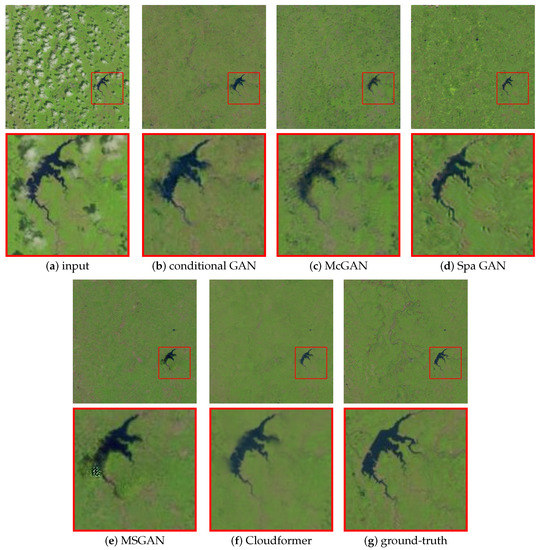
Figure 11.
Comparative experimental results on the first sample of RICE2. When clouds in the image appear as small blocks, conditional GAN and MSGAN cannot remove cloud shadows well. Some white pixels also appear in the results of MSGAN, destroying the continuity of the image. The image recovered by McGAN is too blurry in the outline of the lake, while the result of Spa GAN has many erroneous textures. Our method successfully removes clouds and cloud shadows, outperforming other methods in terms of image texture and continuity.
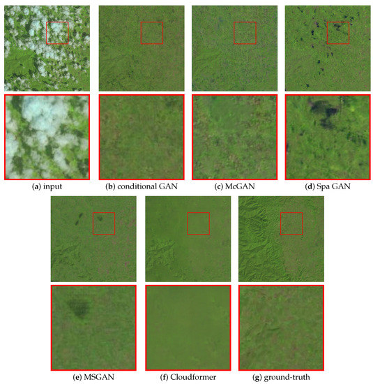
Figure 12.
Comparative experimental results on the second sample of RICE2. When there are medium-sized clouds in the image, Spa GAN and MSGAN produce black blocks. Conditional GAN cannot completely remove cloud shadows. The result of McGAN shows a lot of color distortion. In contrast, our method maintains the tonal consistency of the image.
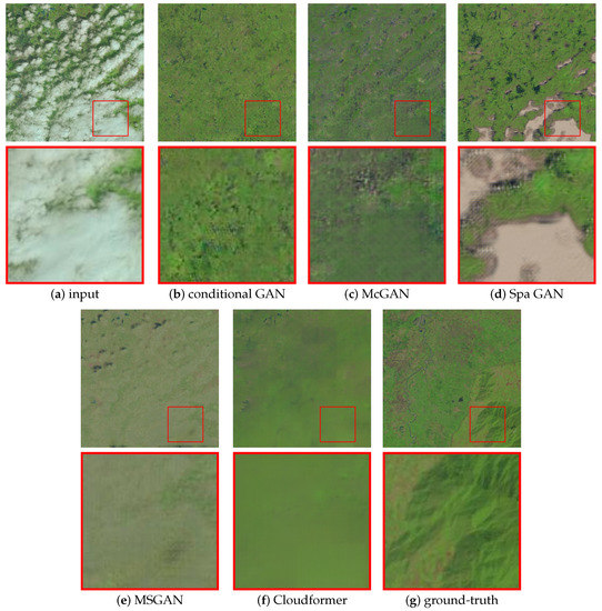
Figure 13.
Comparative experimental results on the third sample of RICE2. When most of the input image is covered by cloud, McGAN, Spa GAN and MSGAN can only preserve color well near areas not obscured by cloud and show a wide range of color distortions in other areas. Conditional GAN produces black patches that destroy image continuity. Relying on only a few cloud-free areas, our method recovers the color information of the entire image as much as possible and maintains image continuity.
From Figure 12, it can be seen that when there are medium-sized clouds in the image, Spa GAN and MSGAN produce black blocks, which may be due to the limited receptive field of the convolution that cannot rely on a wider range of information to complement the occluded regions. As can be seen from the dark spot in the upper right corner of the close-up of the conditional GAN result, it is still difficult to remove cloud shadows well. The result of McGAN shows a lot of color distortion, indicating that it cannot maintain color consistency. In contrast, due to the large receptive field of self-attention, our method maintains the tonal consistency of the image by relying on information from regions not obscured by clouds. Figure 13 represents the case where most of the image is covered by clouds. Convolutional networks often exhibit a wide range of color distortions, probably due to their limited receptive fields. From the close-up of the results of McGAN, Spa GAN and MSGAN, it can be seen that they preserve color well only near areas not obscured by clouds. Although recovering relatively well in terms of color, Conditional GAN produces black patches that destroy image continuity. Relying on only a few cloud-free areas, our method recovers the color information of the entire image as much as possible and maintains image continuity.
4.6. Inference Speed
We calculate the average inference speed of the Cloudformer and the four compared methods on the RICE1 test set. As shown in Table 5, the inference speed of Cloudformer is slower than other methods due to the large amount of computation brought by the transformer structure. In general, however, the speed gap between Cloudformer and other compared methods is acceptable. Considering that cloud-removal tasks usually do not have high speed requirements, it is worth sacrificing some speed for high image quality.

Table 5.
Average inference speed on RICE1 test set.
4.7. Additional Dataset
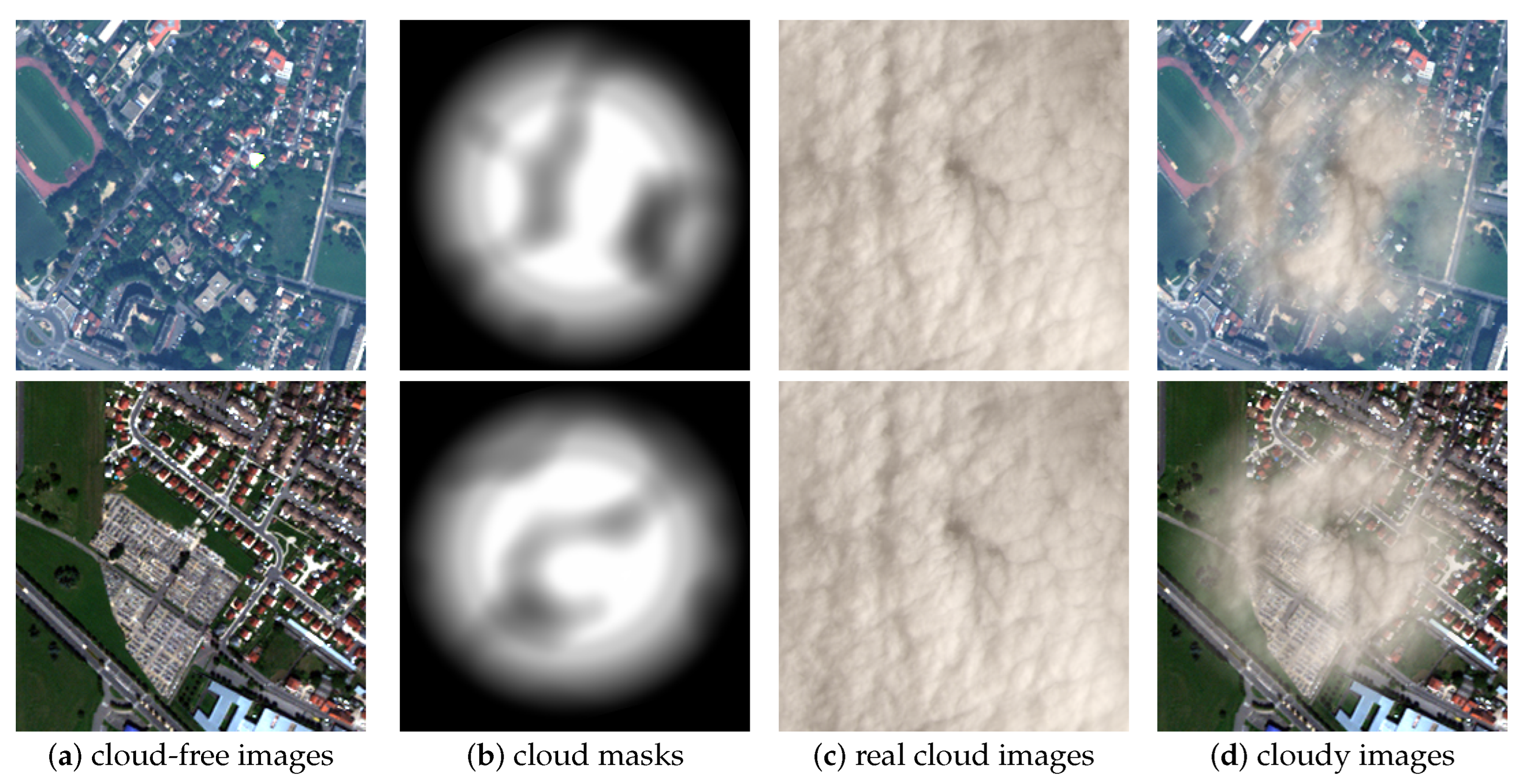
The RICE dataset is mainly collected from natural areas. As a complement, it is necessary to test the algorithm’s performance in more heterogeneous areas such as urban areas. We conduct comparative experiments on the Paris dataset proposed by [64]. The cloud-free images are obtained from WorldView-2 European Cities. The cloudy image () is synthesized from the cloud-free image (), the cloud mask () and the real cloud image () in the following way:
In order to show the synthesis process more intuitively, two samples in the dataset are shown in Figure 14. The Paris dataset contains 4043 samples with a size of 256*256. We select 800 pairs of images from the samples and conduct comparative experiments according to the scheme in Section 4.1.
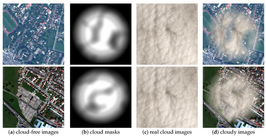
Figure 14.
Two samples from the Paris dataset.
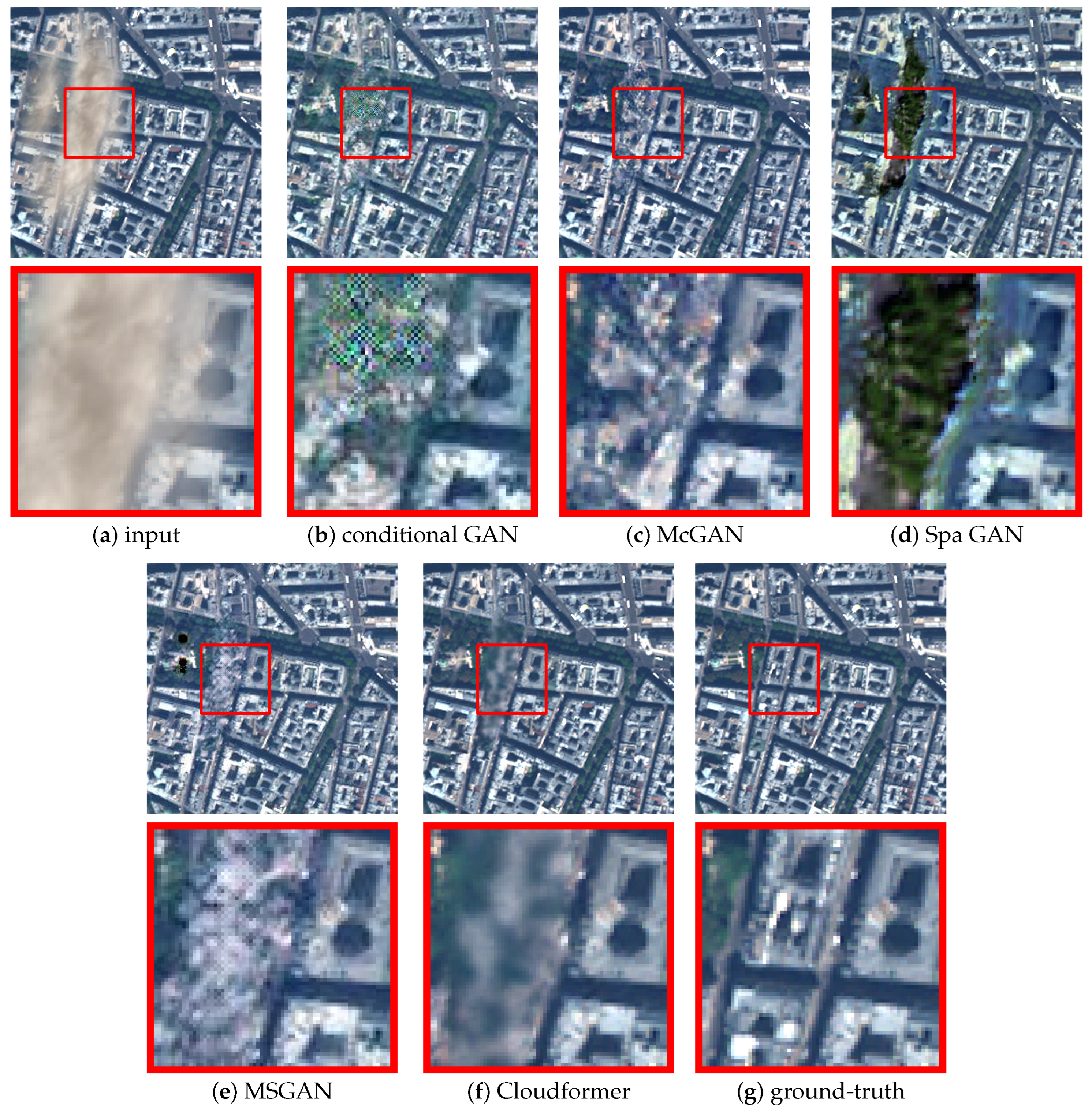
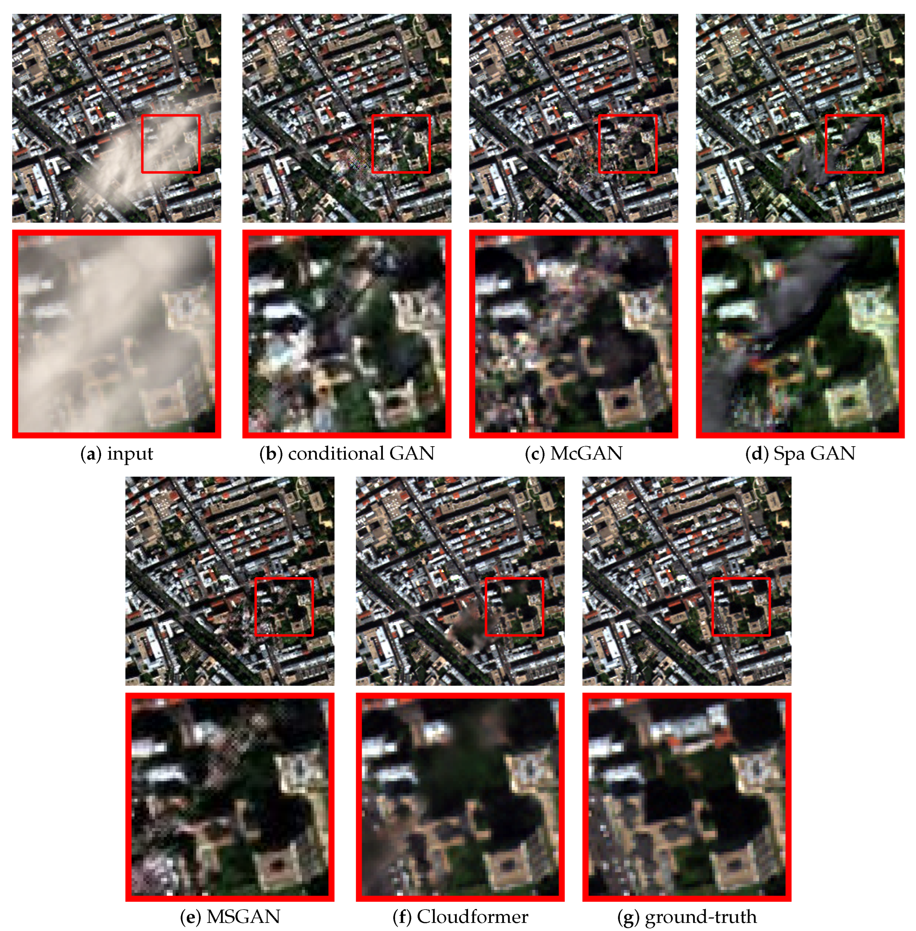
As shown in Table 6, Cloudformer significantly outperforms other comparable methods on quantitative indicators. Our method outperforms the second-best result by 2.897 on PSNR and 0.031 on SSIM. Figure 15 and Figure 16 show the cloud-removal effect of two samples. It can be seen that by benefiting from the flexibility and powerful fitting ability of the transformer structure, the results of our proposed method are superior to the other compared methods in terms of image texture and color.

Table 6.
Quantitative evaluation on Paris dataset.

Figure 15.
Comparative experimental results on first sample of Paris dataset. The result of Cloudformer is closer to the ground-truth than the other compared methods in both texture and color.
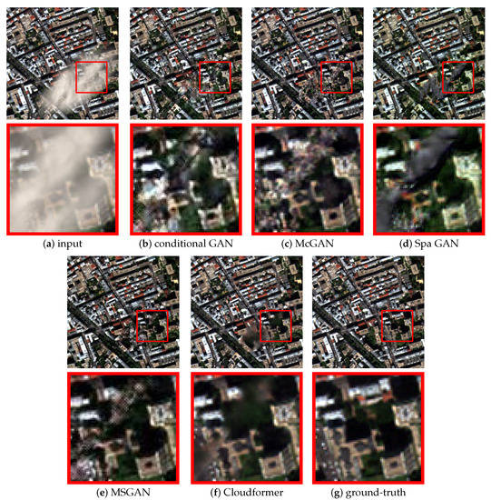
Figure 16.
Comparative experimental results on second sample of Paris dataset. The result of Cloudformer is closer to the ground-truth than other compared methods in both texture and color.
5. Conclusions
In this paper, we propose a novel transformer-based de-clouding network: Cloudformer. Based on previous study and analysis of the self-attention mechanism, we find that in the transformer-based de-cloud network architecture, the shallow self-attention mechanism only produces significant weights in small neighborhoods. Therefore, the shallow self-attention mechanism does not effectively take advantage of its ability to compute dependencies in a large range but instead brings redundant computation and parameters, thus reducing the performance of the network. To solve this problem, our network combines the advantages of convolution and the self-attention mechanism—using convolution in the shallow layer to extract simple features over a small range and using window-based multi-head self-attention in the deep layer to efficiently compute dependencies in a large range to extract more complex features. We also introduce Locally-enhanced Positional Encoding (LePE) in SACB, which enables the network to adaptively generate positional encodings and effectively utilize local information. Experiments on thin-cloud and thick-cloud datasets show that our proposed method significantly outperforms other comparative methods. We also experimentally verify the effectiveness of the proposed module and study the trade-off between convolution and self-attention.
In future research, we will explore application of the transformer structure to cloud removal on multi-temporal and multi-source remote-sensing images and will combine the characteristics of remote-sensing images and the advantages of transformers to study better cloud-removal network architectures.
Author Contributions
P.W. and Z.P. conceived and designed the experiments; H.T., Y.H. and Z.P. contributed materials and computing resources; P.W. performed the experiments and analyzed the results; P.W. wrote the original draft preparation; Z.P. checked the experimental data, examined the experimental results and revised the original draft. All authors have read and agreed to the published version of the manuscript.
Funding
This work was supported by the Youth Innovation Promotion Association, CAS, under number 2022119.
Data Availability Statement
The RICE dataset is available at https://github.com/BUPTLdy/RICE_DATASET (accessed on 7 May 2022). The Paris dataset is available at https://data.mendeley.com/datasets/jk3wr7crj7/3 (accessed on 12 November 2022).
Conflicts of Interest
The authors declare no conflict of interest.
References
- Maggiori, E.; Tarabalka, Y.; Charpiat, G.; Alliez, P. Can semantic labeling methods generalize to any city? the inria aerial image labeling benchmark. In Proceedings of the 2017 IEEE International Geoscience and Remote Sensing Symposium (IGARSS), Worth, TX, USA, 23–28 July 2017; pp. 3226–3229. [Google Scholar]
- Vogelmann, J.E.; Tolk, B.; Zhu, Z. Monitoring forest changes in the southwestern United States using multitemporal Landsat data. Remote Sens. Environ. 2009, 113, 1739–1748. [Google Scholar] [CrossRef]
- King, M.D.; Platnick, S.; Menzel, W.P.; Ackerman, S.A.; Hubanks, P.A. Spatial and temporal distribution of clouds observed by MODIS onboard the Terra and Aqua satellites. IEEE Trans. Geosci. Remote Sens. 2013, 51, 3826–3852. [Google Scholar] [CrossRef]
- Dosovitskiy, A.; Beyer, L.; Kolesnikov, A.; Weissenborn, D.; Zhai, X.; Unterthiner, T.; Dehghani, M.; Minderer, M.; Heigold, G.; Gelly, S.; et al. An image is worth 16×16 words: Transformers for image recognition at scale. arXiv 2020, arXiv:2010.11929. [Google Scholar]
- Chen, H.; Wang, Y.; Guo, T.; Xu, C.; Deng, Y.; Liu, Z.; Ma, S.; Xu, C.; Xu, C.; Gao, W. Pre-trained image processing transformer. In Proceedings of the IEEE/CVF Conference on Computer Vision and Pattern Recognition, Nashville, TN, USA, 19–25 June 2021; pp. 12299–12310. [Google Scholar]
- Zamir, S.W.; Arora, A.; Khan, S.; Hayat, M.; Khan, F.S.; Yang, M.H. Restormer: Efficient transformer for high-resolution image restoration. In Proceedings of the IEEE/CVF Conference on Computer Vision and Pattern Recognition, New Orleans, LA, USA, 19–20 June 2022; pp. 5728–5739. [Google Scholar]
- Carion, N.; Massa, F.; Synnaeve, G.; Usunier, N.; Kirillov, A.; Zagoruyko, S. End-to-end object detection with transformers. In Proceedings of the European Conference on Computer Vision, Glasgow, UK, 23–28 August 2020; Springer: Berlin/Heidelberg, Germany, 2020; pp. 213–229. [Google Scholar]
- Zhu, X.; Su, W.; Lu, L.; Li, B.; Wang, X.; Dai, J. Deformable detr: Deformable transformers for end-to-end object detection. arXiv 2020, arXiv:2010.04159. [Google Scholar]
- Wang, Y.; Xu, Z.; Wang, X.; Shen, C.; Cheng, B.; Shen, H.; Xia, H. End-to-end video instance segmentation with transformers. In Proceedings of the IEEE/CVF Conference on Computer Vision and Pattern Recognition, Nashville, TN, USA, 19–25 June 2021; pp. 8741–8750. [Google Scholar]
- Zheng, S.; Lu, J.; Zhao, H.; Zhu, X.; Luo, Z.; Wang, Y.; Fu, Y.; Feng, J.; Xiang, T.; Torr, P.H.; et al. Rethinking semantic segmentation from a sequence-to-sequence perspective with transformers. In Proceedings of the IEEE/CVF Conference on Computer Vision and Pattern Recognition, Nashville, TN, USA, 19–25 June 2021; pp. 6881–6890. [Google Scholar]
- Vaswani, A.; Shazeer, N.; Parmar, N.; Uszkoreit, J.; Jones, L.; Gomez, A.N.; Kaiser, Ł.; Polosukhin, I. Attention is all you need. In Advances in Neural Information Processing Systems; MIT Press: Cambridge, MA, USA, 2017; Volume 30. [Google Scholar]
- Dong, X.; Bao, J.; Chen, D.; Zhang, W.; Yu, N.; Yuan, L.; Chen, D.; Guo, B. Cswin transformer: A general vision transformer backbone with cross-shaped windows. In Proceedings of the IEEE/CVF Conference on Computer Vision and Pattern Recognition, New Orleans, LA, USA, 19–20 June 2022; pp. 12124–12134. [Google Scholar]
- Lin, C.H.; Tsai, P.H.; Lai, K.H.; Chen, J.Y. Cloud removal from multitemporal satellite images using information cloning. IEEE Trans. Geosci. Remote Sens. 2012, 51, 232–241. [Google Scholar] [CrossRef]
- Cheng, Q.; Shen, H.; Zhang, L.; Yuan, Q.; Zeng, C. Cloud removal for remotely sensed images by similar pixel replacement guided with a spatio-temporal MRF model. ISPRS J. Photogramm. Remote Sens. 2014, 92, 54–68. [Google Scholar] [CrossRef]
- Li, X.; Shen, H.; Zhang, L.; Zhang, H.; Yuan, Q.; Yang, G. Recovering quantitative remote sensing products contaminated by thick clouds and shadows using multitemporal dictionary learning. IEEE Trans. Geosci. Remote Sens. 2014, 52, 7086–7098. [Google Scholar]
- Chen, B.; Huang, B.; Chen, L.; Xu, B. Spatially and temporally weighted regression: A novel method to produce continuous cloud-free Landsat imagery. IEEE Trans. Geosci. Remote Sens. 2016, 55, 27–37. [Google Scholar] [CrossRef]
- Wen, F.; Zhang, Y.; Gao, Z.; Ling, X. Two-pass robust component analysis for cloud removal in satellite image sequence. IEEE Geosci. Remote Sens. Lett. 2018, 15, 1090–1094. [Google Scholar] [CrossRef]
- Ji, T.Y.; Chu, D.; Zhao, X.L.; Hong, D. A unified framework of cloud detection and removal based on low-rank and group sparse regularizations for multitemporal multispectral images. IEEE Trans. Geosci. Remote Sens. 2022, 60, 1–15. [Google Scholar] [CrossRef]
- Eckardt, R.; Berger, C.; Thiel, C.; Schmullius, C. Removal of optically thick clouds from multi-spectral satellite images using multi-frequency SAR data. Remote Sens. 2013, 5, 2973–3006. [Google Scholar] [CrossRef]
- Zhu, C.; Zhao, Z.; Zhu, X.; Nie, Z.; Liu, Q.H. Cloud removal for optical images using SAR structure data. In Proceedings of the 2016 IEEE 13th International Conference on Signal Processing (ICSP), Chengdu, China, 6–10 November 2016; pp. 1872–1875. [Google Scholar]
- Li, Y.; Li, W.; Shen, C. Removal of optically thick clouds from high-resolution satellite imagery using dictionary group learning and interdictionary nonlocal joint sparse coding. IEEE J. Sel. Top. Appl. Earth Obs. Remote Sens. 2017, 10, 1870–1882. [Google Scholar] [CrossRef]
- Li, W.; Li, Y.; Chan, J.C.W. Thick cloud removal with optical and SAR imagery via convolutional-mapping-deconvolutional network. IEEE Trans. Geosci. Remote Sens. 2019, 58, 2865–2879. [Google Scholar] [CrossRef]
- Meng, Q.; Borders, B.E.; Cieszewski, C.J.; Madden, M. Closest spectral fit for removing clouds and cloud shadows. Photogramm. Eng. Remote Sens. 2009, 75, 569–576. [Google Scholar] [CrossRef]
- Chavez Jr, P.S. An improved dark-object subtraction technique for atmospheric scattering correction of multispectral data. Remote Sens. Environ. 1988, 24, 459–479. [Google Scholar] [CrossRef]
- Zhang, Y.; Guindon, B.; Cihlar, J. An image transform to characterize and compensate for spatial variations in thin cloud contamination of Landsat images. Remote Sens. Environ. 2002, 82, 173–187. [Google Scholar] [CrossRef]
- He, X.Y.; Hu, J.B.; Chen, W.; Li, X.Y. Haze removal based on advanced haze-optimized transformation (AHOT) for multispectral imagery. Int. J. Remote Sens. 2010, 31, 5331–5348. [Google Scholar] [CrossRef]
- Du, Y.; Guindon, B.; Cihlar, J. Haze detection and removal in high resolution satellite image with wavelet analysis. IEEE Trans. Geosci. Remote Sens. 2002, 40, 210–217. [Google Scholar]
- Siravenha, A.C.; Sousa, D.; Bispo, A.; Pelaes, E. The use of high-pass filters and the inpainting method to clouds removal and their impact on satellite images classification. In Proceedings of the International Conference on Image Analysis and Processing, Ravenna, Italy, 14–16 September 2011; Springer: Berlin/Heidelberg, Germany, 2011; pp. 333–342. [Google Scholar]
- Shen, H.; Li, H.; Qian, Y.; Zhang, L.; Yuan, Q. An effective thin cloud removal procedure for visible remote sensing images. ISPRS J. Photogramm. Remote Sens. 2014, 96, 224–235. [Google Scholar] [CrossRef]
- Xu, M.; Jia, X.; Pickering, M. Automatic cloud removal for Landsat 8 OLI images using cirrus band. In Proceedings of the 2014 IEEE Geoscience and Remote Sensing Symposium, Quebec City, QC, Canada, 13–18 July 2014; pp. 2511–2514. [Google Scholar]
- Xu, M.; Pickering, M.; Plaza, A.J.; Jia, X. Thin cloud removal based on signal transmission principles and spectral mixture analysis. IEEE Trans. Geosci. Remote Sens. 2015, 54, 1659–1669. [Google Scholar] [CrossRef]
- He, K.; Sun, J.; Tang, X. Single image haze removal using dark channel prior. IEEE Trans. Pattern Anal. Mach. Intell. 2010, 33, 2341–2353. [Google Scholar] [PubMed]
- Li, W.; Li, Y.; Chen, D.; Chan, J.C.W. Thin cloud removal with residual symmetrical concatenation network. ISPRS J. Photogramm. Remote Sens. 2019, 153, 137–150. [Google Scholar] [CrossRef]
- Wang, X.; Xu, G.; Wang, Y.; Lin, D.; Li, P.; Lin, X. Thin and thick cloud removal on remote sensing image by conditional generative adversarial network. In Proceedings of the IGARSS 2019-2019 IEEE International Geoscience and Remote Sensing Symposium, Yokohama, Japan, 28 July–2 August 2019; pp. 1426–1429. [Google Scholar]
- Isola, P.; Zhu, J.Y.; Zhou, T.; Efros, A.A. Image-to-image translation with conditional adversarial networks. In Proceedings of the IEEE Conference on Computer Vision and Pattern Recognition, Honolulu, HI, USA, 21–26 July 2017; pp. 1125–1134. [Google Scholar]
- Enomoto, K.; Sakurada, K.; Wang, W.; Fukui, H.; Matsuoka, M.; Nakamura, R.; Kawaguchi, N. Filmy cloud removal on satellite imagery with multispectral conditional generative adversarial nets. In Proceedings of the IEEE Conference on Computer Vision and Pattern Recognition Workshops, Honolulu, HI, USA, 21–26 July 2017; pp. 48–56. [Google Scholar]
- Pan, H. Cloud removal for remote sensing imagery via spatial attention generative adversarial network. arXiv 2020, arXiv:2009.13015. [Google Scholar]
- Xu, M.; Deng, F.; Jia, S.; Jia, X.; Plaza, A.J. Attention mechanism-based generative adversarial networks for cloud removal in Landsat images. Remote Sens. Environ. 2022, 271, 112902. [Google Scholar] [CrossRef]
- Zhu, J.Y.; Park, T.; Isola, P.; Efros, A.A. Unpaired image-to-image translation using cycle-consistent adversarial networks. In Proceedings of the IEEE International Conference on Computer Vision, Venice, Italy, 22–29 October 2017; pp. 2223–2232. [Google Scholar]
- Singh, P.; Komodakis, N. Cloud-gan: Cloud removal for sentinel-2 imagery using a cyclic consistent generative adversarial networks. In Proceedings of the IGARSS 2018-2018 IEEE International Geoscience and Remote Sensing Symposium, Valencia, Spain, 22–27 July 2018; pp. 1772–1775. [Google Scholar]
- Li, J.; Wu, Z.; Hu, Z.; Zhang, J.; Li, M.; Mo, L.; Molinier, M. Thin cloud removal in optical remote sensing images based on generative adversarial networks and physical model of cloud distortion. ISPRS J. Photogramm. Remote Sens. 2020, 166, 373–389. [Google Scholar] [CrossRef]
- Liu, L.; Hu, S. SACTNet: Spatial Attention Context Transformation Network for Cloud Removal. Wirel. Commun. Mob. Comput. 2021, 2021, 8292612. [Google Scholar] [CrossRef]
- Christopoulos, D.; Ntouskos, V.; Karantzalos, K. Cloudtran: Cloud removal from multitemporal satellite images using axial transformer networks. Int. Arch. Photogramm. Remote Sens. Spat. Inf. Sci. 2022, 43, 1125–1132. [Google Scholar] [CrossRef]
- Wu, H.; Xiao, B.; Codella, N.; Liu, M.; Dai, X.; Yuan, L.; Zhang, L. Cvt: Introducing convolutions to vision transformers. In Proceedings of the IEEE/CVF International Conference on Computer Vision, Montreal, QC, Canada, 10–17 October 2021; pp. 22–31. [Google Scholar]
- Li, Y.; Zhang, K.; Cao, J.; Timofte, R.; Van Gool, L. Localvit: Bringing locality to vision transformers. arXiv 2021, arXiv:2104.05707. [Google Scholar]
- Yuan, K.; Guo, S.; Liu, Z.; Zhou, A.; Yu, F.; Wu, W. Incorporating convolution designs into visual transformers. In Proceedings of the IEEE/CVF International Conference on Computer Vision, Montreal, QC, Canada, 10–17 October 2021; pp. 579–588. [Google Scholar]
- Li, K.; Wang, Y.; Zhang, J.; Gao, P.; Song, G.; Liu, Y.; Li, H.; Qiao, Y. Uniformer: Unifying convolution and self-attention for visual recognition. arXiv 2022, arXiv:2201.09450. [Google Scholar]
- Huang, Z.; Ben, Y.; Luo, G.; Cheng, P.; Yu, G.; Fu, B. Shuffle transformer: Rethinking spatial shuffle for vision transformer. arXiv 2021, arXiv:2106.03650. [Google Scholar]
- Chu, X.; Tian, Z.; Wang, Y.; Zhang, B.; Ren, H.; Wei, X.; Xia, H.; Shen, C. Twins: Revisiting the design of spatial attention in vision transformers. Adv. Neural Inf. Process. Syst. 2021, 34, 9355–9366. [Google Scholar]
- Liu, Z.; Lin, Y.; Cao, Y.; Hu, H.; Wei, Y.; Zhang, Z.; Lin, S.; Guo, B. Swin transformer: Hierarchical vision transformer using shifted windows. In Proceedings of the IEEE/CVF International Conference on Computer Vision, Montreal, QC, Canada, 10–17 October 2021; pp. 10012–10022. [Google Scholar]
- Vaswani, A.; Ramachandran, P.; Srinivas, A.; Parmar, N.; Hechtman, B.; Shlens, J. Scaling local self-attention for parameter efficient visual backbones. In Proceedings of the IEEE/CVF Conference on Computer Vision and Pattern Recognition, Nashville, TN, USA, 19–25 June 2021; pp. 12894–12904. [Google Scholar]
- Gehring, J.; Auli, M.; Grangier, D.; Yarats, D.; Dauphin, Y.N. Convolutional sequence to sequence learning. In Proceedings of the International Conference on Machine Learning, PMLR, Sydney, Australia, 6–11 August 2017; pp. 1243–1252. [Google Scholar]
- Shaw, P.; Uszkoreit, J.; Vaswani, A. Self-attention with relative position representations. arXiv 2018, arXiv:1803.02155. [Google Scholar]
- Dai, Z.; Yang, Z.; Yang, Y.; Carbonell, J.; Le, Q.V.; Salakhutdinov, R. Transformer-xl: Attentive language models beyond a fixed-length context. arXiv 2019, arXiv:1901.02860. [Google Scholar]
- Raffel, C.; Shazeer, N.; Roberts, A.; Lee, K.; Narang, S.; Matena, M.; Zhou, Y.; Li, W.; Liu, P.J. Exploring the limits of transfer learning with a unified text-to-text transformer. J. Mach. Learn. Res. 2020, 21, 1–67. [Google Scholar]
- He, P.; Liu, X.; Gao, J.; Chen, W. Deberta: Decoding-enhanced bert with disentangled attention. arXiv 2020, arXiv:2006.03654. [Google Scholar]
- Chu, X.; Tian, Z.; Zhang, B.; Wang, X.; Wei, X.; Xia, H.; Shen, C. Conditional positional encodings for vision transformers. arXiv 2021, arXiv:2102.10882. [Google Scholar]
- Wang, Z.; Cun, X.; Bao, J.; Zhou, W.; Liu, J.; Li, H. Uformer: A general u-shaped transformer for image restoration. In Proceedings of the IEEE/CVF Conference on Computer Vision and Pattern Recognition, New Orleans, LA, USA, 19–20 June 2022; pp. 17683–17693. [Google Scholar]
- Charbonnier, P.; Blanc-Feraud, L.; Aubert, G.; Barlaud, M. Two deterministic half-quadratic regularization algorithms for computed imaging. In Proceedings of the 1st International Conference on Image Processing, Austin, TX, USA, 13–16 November 1994; Volume 2, pp. 168–172. [Google Scholar]
- Zamir, S.W.; Arora, A.; Khan, S.; Hayat, M.; Khan, F.S.; Yang, M.H.; Shao, L. Learning enriched features for real image restoration and enhancement. In Proceedings of the European Conference on Computer Vision, Glasgow, UK, 23–28 August 2020; Springer: Berlin/Heidelberg, Germany, 2020; pp. 492–511. [Google Scholar]
- Lin, D.; Xu, G.; Wang, X.; Wang, Y.; Sun, X.; Fu, K. A remote sensing image dataset for cloud removal. arXiv 2019, arXiv:1901.00600. [Google Scholar]
- Loshchilov, I.; Hutter, F. Decoupled weight decay regularization. arXiv 2017, arXiv:1711.05101. [Google Scholar]
- Zhou, J.; Luo, X.; Rong, W.; Xu, H. Cloud Removal for Optical Remote Sensing Imagery Using Distortion Coding Network Combined with Compound Loss Functions. Remote Sens. 2022, 14, 3452. [Google Scholar] [CrossRef]
- Hasan, C.; Horne, R.; Mauw, S.; Mizera, A. Cloud removal from satellite imagery using multispectral edge-filtered conditional generative adversarial networks. Int. J. Remote Sens. 2022, 43, 1881–1893. [Google Scholar] [CrossRef]
Publisher’s Note: MDPI stays neutral with regard to jurisdictional claims in published maps and institutional affiliations. |
© 2022 by the authors. Licensee MDPI, Basel, Switzerland. This article is an open access article distributed under the terms and conditions of the Creative Commons Attribution (CC BY) license (https://creativecommons.org/licenses/by/4.0/).

