Assessing Elevation-Based Forest Dynamics over Space and Time toward REDD+ MRV in Upland Myanmar

Abstract

Implementation of a measuring, reporting, and verifying (MRV) framework is essential for reducing emissions from deforestation and forest degradation (REDD+). According to the United Nations Framework Convention on Climate Change, MRV can be regarded as an important mechanism to mitigate global warming. Upland Myanmar, with an elevation of ~80–2600 m, is experiencing tropical deforestation, which is commonly explained by the expansion of shifting cultivation. The vegetation change tracker algorithm, with its high-automation and wild-adaptation features, and the enhanced integrated forest z-score were applied in this elevation-based study of time series deforestation monitoring in upland Myanmar using data from 2003 to 2015. Four spatial patterns of deforestation, namely stripes, adjacent, filled, and staggered, were found in the research area. Moreover, our work showed that the center of elevation of deforestation was ~1000 m. Further analysis revealed that this center tended to shift to a higher elevation over time; a “golden cross”/changeover could be deciphered at ~1000 m, indicating that the scale and intensity of shifting cultivation continue to expand vertically. The results suggest the need to track the elevation-based signature of vegetation clearings to help achieve the goals of REDD+ at the regional level in tropical rainforest countries.

1. Introduction

According to the assessment report of the United Nations Intergovernmental Panel on Climate Change (IPCC), deforestation and related activities have become the second largest emission source of greenhouse gas (GHG) emissions, accounting for ~17%–24% of the total global GHG emissions [1,2]. Tropical areas, which are home to large forests, are experiencing rapid population growth and strong economic demand. Thus, the problems of deforestation and forest degradation are more serious in such areas [3,4,5]. These behaviors are directly responsible for an extremely rapid disappearance of tropical forests with a rate of ~13 million hm² every year and global annual anthropogenic carbon emissions of up to 12% [6]. Therefore, reducing emissions from deforestation and degradation (REDD+) was proposed at the 11th UN Climate Change Conference in 2005 as an important element of mitigating climate change and increasing carbon sequestration [7,8,9,10].

REDD+ is a part of the overall global action for climate change mitigation. It aims to raise funds from developed countries every year to help their developing counterparts reduce GHG emissions caused by deforestation [8,11,12]. Mandel and other experts have shown that REDD+ and other global emission reduction actions could help reduce up to 3.76 billion tons of carbon dioxide emissions per year, eventually reaching 100 billion tons by 2030 [13,14,15]. As per IPCC’s assessment, REDD+ can not only achieve a greater emission reduction effect but also protect large forests and their biodiversity. Transparent, accountable, and sustainable monitoring, reporting, and verification (MRV) systems are essential for any REDD+ framework. With the prospect of a global agreement on forest preservation on the horizon, establishing functional MRV systems is one of the major goals of so called ‘REDD Readiness’ [16]. Furthermore, with REDD+ looking increasingly likely to become operational in the coming years, there is a significant demand for MRV best practice, holistically including carbon, biodiversity, social, and ecosystem service monitoring [17,18].

As one of the main targets under the REDD+ MRV framework, Myanmar covers an area of 678,500 km² and has a forest coverage rate of over 55% [19,20,21]. Such a large forest area not only stores a considerable amount of carbon but is also home to irreplaceable local biodiversity [22,23]. Simultaneously, it serves as an important source of livelihood for the Myanmarese population [24]. However, local agricultural economic activities based on forests are also the main driving forces of carbon emissions generation and biodiversity loss [25,26]. Each year from 2001 to 2010, the total deforestation area in Myanmar was calculated as 21,178.8 km², resulting in an annual deforestation rate of 0.81% [27]. The total forest carbon release was 20.06 million tons and the annual deforestation rate was 0.37%. The annual average of the disturbed forest area in Myanmar is 336,000 hm2, ranking second in Southeast Asia [27].

According to a survey, forest loss in Myanmar was mainly caused by the expansion of shifting cultivation, illegal logging, and wildfire, among which the expansion of shifting cultivation was pinpointed by the Forest Department of Myanmar as the main underlying cause of deforestation [28,29]. Shifting cultivation is a unique local farming method that differs from conventional agricultural practices and is very common in upland Myanmar. Traditional shifting cultivation involves felling, cultivation, and restoration, thus following a sustainable agricultural circular economy model [30,31,32]. The shifting cultivation process comprises three phases: first, the primary forest is cut down and burned as fertilizer for the reclaimed farmland; this is called the burning phase [33,34]. Second, crops of various types are planted on the cleared farmland; this is called the cropping phase. Finally, after the farmland is no longer fertile, it is kept idle to allow vegetation regeneration; this is called the fallow phase. During the last phase, farmers plant crops in other plots, and at the end of this particular cropping phase, they clear the regenerated secondary forest on the original plots [35]. Typically, the fallow phase period can extend over more than 30 years, allowing complete regeneration of secondary forests in tropical areas [36]. However, due to various socio-economic factors, including population growth, market development, and government policies, the traditional agricultural economic cycle has been broken in many plots [37]. For example, the fallow phase in many plots may last for only 2–3 years, which is insufficient for forest regeneration. Moreover, farmland in many areas has been overused for a long time and has lost the capability to restore secondary forests [38]. These changes exacerbate the felling of primary forests and lead to a growth in carbon emissions and local biodiversity loss [39].

Due to the topography of upland Myanmar, deforestation in the country is largely affected by elevation [40,41]. Elevation impacts deforestation activities in Myanmar primarily in two ways. First, elevation affects human activity. The distribution of the human population in Myanmar varies significantly at different elevations, and this aspect partially determines the basis of deforestation [42,43]. Furthermore, the forests in Myanmar are distributed at different elevations, showing varied distribution patterns [44]. The forest type changes with elevation. Different tree species cause various effects on soil fertility during the burning phase of shifting cultivation [45,46]. Notably, the influence of human activities, climate, and other factors in various elevation segments lead to differences in the distributions of natal forests and secondary forests [47,48]. Within the same elevation segment, primeval forests bear a greater risk of deforestation [49].

Although a considerable amount of research refers to shifting cultivation in Myanmar, the literature has only a few examples of systematic research on the effects of the intensity distribution of deforestation by elevation due to shifting cultivation expansion activities in upland Myanmar [50,51,52]. Moreover, the rapid population increase in Myanmar during recent years has exacerbated the intensity of shifting cultivation as well as expanded the scope of human activities [53]. Therefore, academics and practitioners devoted to forest research in upland Myanmar face new questions: what is the spatial expansion pattern of shifting cultivation in upland Myanmar? How does elevation affect expansion? To solve these problems, we used a highly automated change detection algorithm, called the vegetation change tracker (VCT), to analyze what we called the enhanced integrated forest z-score (IFZ). The purpose of this research was to accomplish elevation-based identification and estimation of deforestation in the study area. The results of this work may provide a reference for identifying, assessing, and prioritizing all drivers of deforestation and forest degradation in the REDD+ measuring, reporting, and verifying (MRV) framework.

2. Materials and Methods

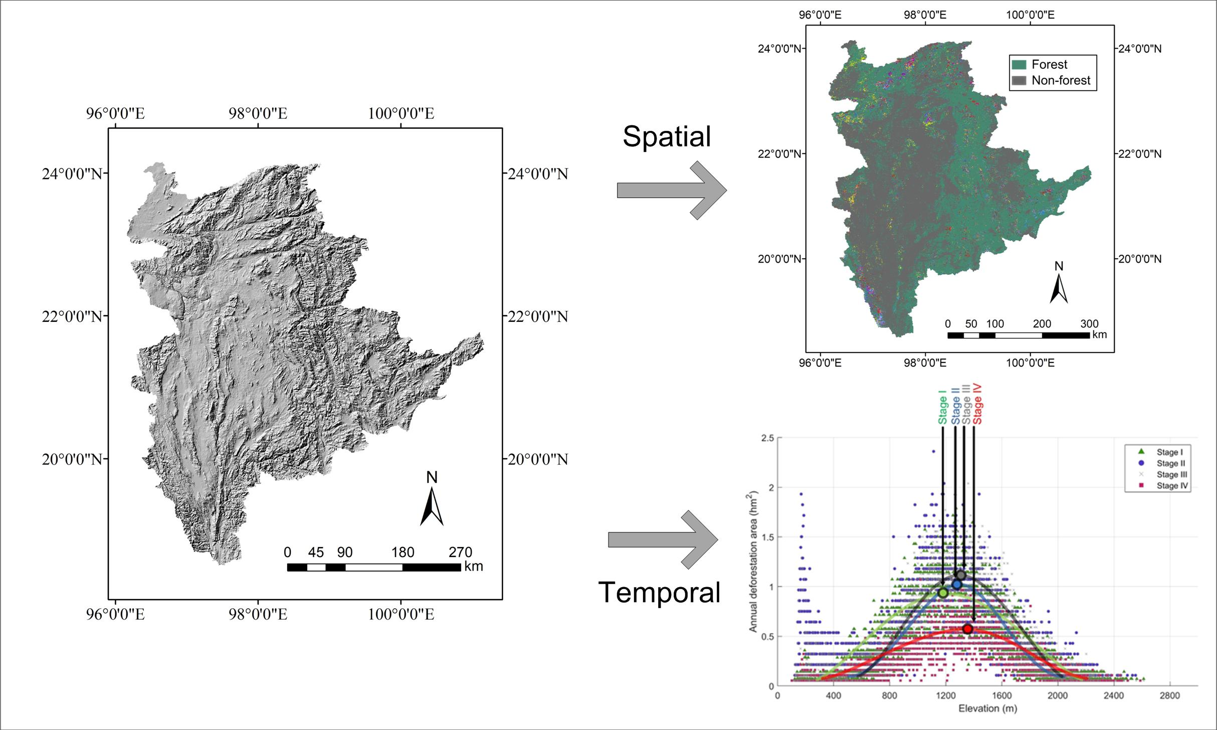
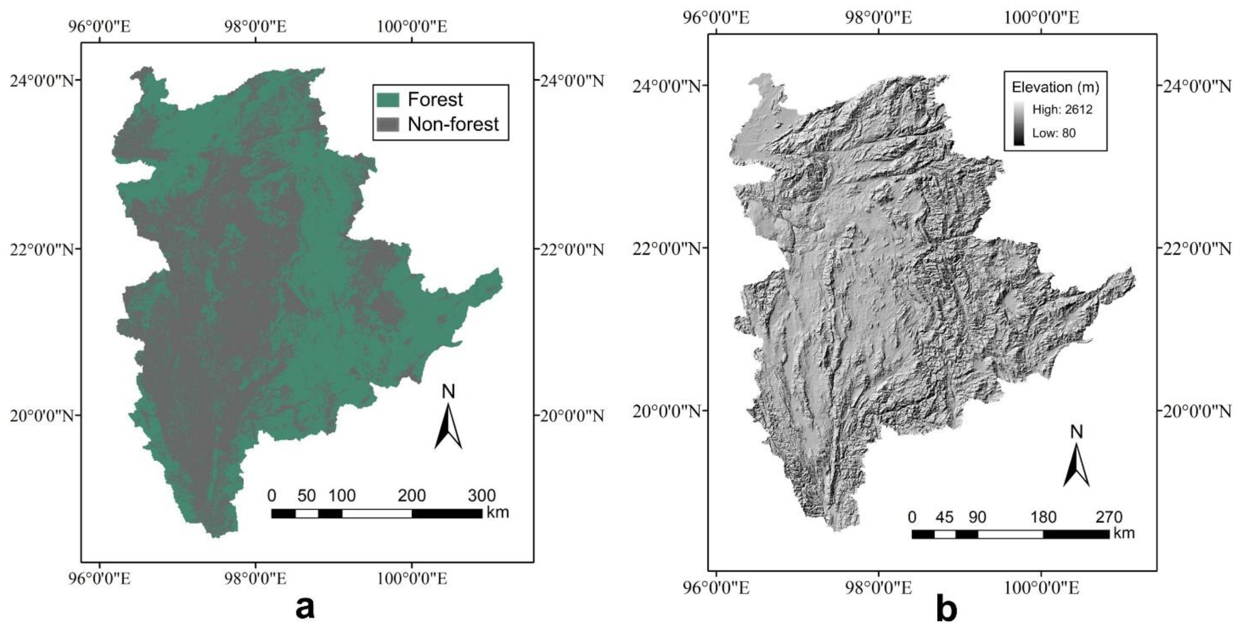
2.1. Research Area

Our research area, upland Myanmar, is located in northeastern Myanmar (Figure 1). The elevation distribution of this area ranges from 80 m to more than 2600 m, with an average elevation of 1000–1200 m [37]. The climate in this area is mainly of the tropical monsoon type, with three different seasons: the hot season from mid-February to mid-May, the rainy season from mid-May to mid-October, and the cool season from mid-October to mid-February [41,54]. Among them, January is the coldest month with an average temperature of more than 20 °C, and April is the hottest month with an average temperature of ~30 °C [53]. The annual precipitation in most parts of upland Myanmar ranges between 1000 and 2000 mm [55]. Upland Myanmar is home to three mountains and four water systems from the north to the south, and many basins and rivers can be found on the plateau as well [51].

Due to abundant precipitation, suitable topography, and temperature, upland Myanmar hosts one of the most abundant forest resources, not only in the region itself, but also in Southeast Asia. The forest area of upland Myanmar covers an expansive area of 180,000 ha, and the forest coverage rate is ~50% [37]. There are seven types of forests in this area, including deciduous mixed, temperate evergreen, and arid forests [52]. Up to 2088 species of timber trees have been recorded in Myanmar, including 85 species of high-quality and precious timber trees, such as teak, pear, red sandalwood, and Phoebe [56,57].

Interestingly, this area also accounts for 66% of the country’s townships and is home to 42% of the national population [37]. Local forests have been seriously damaged in a quest to meet the economic needs of the continuous and swift population increase. Although the Myanmarese government issued several forest protection policies between 1990 and 2015, forest coverage decreased by 14% [58]. One of the reasons for deforestation is agricultural demand and shifting agriculture accounts for over 70% of the total agricultural area [59,60]. The fallow period in this region varies from 6–27 years. With the rapid development of the economy and road networks, shifting cultivation, and fallow forests are undergoing accelerated transformations [33].

2.2. Data Standardization and Forest Masking

Due to the long time series and a short revisit period, MODIS has been widely used in forest monitoring and mapping worldwide. The MODIS Land Science Team provides a suite of standard MODIS data products to users, including the MODIS Surface Reflectance Product (MOD09A1) and MODIS land cover data (MCD12Q1). Land cover data are obtained from MCD12Q1, a Level 3 product of the MODIS land cover datasets [61]. This product has non-negligible significance in surface research and has been widely used in different application fields. MCD12Q1 contains five data layers corresponding to five different classification schemes [62,63,64]. The data for this work were obtained from the U.S. Geological Survey (USGS) Center for Earth Resources Observation and Science (http://earthexplorer.usgs.gov (accessed on 1 October 2022)), and the acquisition dates of the images range between 2002 and 2016. The MODIS images used in this work have a spatial resolution of 500 m. In addition, elevation data were also acquired from the USGS and used to study the impact of elevation. All the scenes were georeferenced to the Universal Transverse Mercator map projection, WGS 84 datum.

To eliminate the influence of seasonal variation and directional reflection on data consistency, we conducted data standardization as the preprocessing step. In this study, we used the red (620–670 nm) and near-infrared (NIR1: 841–875 nm; NIR2: 1230–1250 nm) bands from the MODIS Surface Reflectance Product (MOD09A1) as follows:

$$I_r=\frac{I-I_{\mu }}{I_{\sigma }}$$

(1)

Among them, I_r is the standardized band or index and I_μ and I_σ are the average and standard deviation of pixel level spectral reflectance for the mature forest area in the band or index, respectively.

A forest mask was used to identify and extract the forest land information in the starting year (2002). Forest identification was based on values from 1 to 7 in the MCD12Q1 data of MODIS, which were obtained from the International Geosphere-Biosphere Program land classification system. These values might include evergreen coniferous forests, evergreen broad-leaved forests, deciduous coniferous forests, deciduous broad-leaved forests, mixed forests, dense shrub forests, and sparse shrub forests. The other values were regarded as belonging to non-forest areas. Finally, the images of the forest and non-forest areas were distinguished after the forest mask processing.

2.3. Integrated Forest Score for Individual Forest Area Description

The principle of the IFZ is based on the forest peak feature selection of dark targets, which uses the performance characteristics of forest pixels in different bands. Therefore, for the upland Myanmar region, pixels in a farmland and the early fallow state will not significantly affect the accuracy of the description provided by the IFZ. Simultaneously, as the IFZ of each pixel in space is also independent, this score can provide a good description of the change in the spatial characteristics of a forest. In other words, the IFZ is the integration of the spectral characteristics of the forest pixels known in each band. To generate the IFZ, a parameter denoted as FZ_i, and called the forest z-score must first be calculated using the spectral signature of known forest pixels within each image to normalize the image. Firstly, for the known forest pixels of band i, the mean of the spectral values is supposed as b_i and the standard deviation is SD_i. Then, the ${\overline{b}}_i$ is the mean of b_i in each band. Finally, for any pixel, b_pi, in that image, FZ_i for that band can be calculated as follows:

$$F{Z}_i=\frac{b_i-{\overline{b}}_i}{S{D}_i}$$

(2)

For multispectral satellite images, the IFZ of each pixel is defined by integrating FZ_i over the spectral bands as follows:

$$IFZ=\sqrt{\frac{1}{NB}{{\displaystyle \sum }}_{i=1}^{NB}{\left(F{Z}_i\right)}^2}$$

(3)

where NB is the number of bands used. It should be noted that one related band, which is a near-infrared band (band 4), is excluded for the reason that the values reflecting non-forest surfaces might show high or low depending on the non-forest cover type while the forest canopy typically presents with high reflectance values in this band. This can be a serious problem for the result as forest disturbances do not necessarily lead to spectral changes in a particular direction in this band, and spectral changes in this band do not definitively indicate real disturbances.

It is worth noting that if the spectral characteristics of the forest pixels have a normal distribution, the probability of pixels being forest pixels, and hence FZ_i, can be calculated with the standardized normal distribution table (SDST) released in the Statistical Yearbook of Forestry. As the root sum square of FZi, IFZ can be interpreted similarly. Although the forest pixels in MODIS images may not provide a strict normal distribution in all bands, the approximate probability interpretations of FZ_i and IFZ allow the use of probability-based thresholds, which may be applicable to images collected at different locations and on various days, for future time series analyses.

An intuitive explanation for the IFZ is that it describes the possibility of a pixel becoming a forest pixel at a certain time. This is an inverse ratio measure; that is, when the IFZ of the pixel at that time is larger, the probability of the pixel being a non-forest pixel is greater. In contrast, when the IFZ of the pixel at that time is smaller (~0), the pixel is closer to the spectral center of the forest sample. Thus, it has a high probability of being a forest pixel.

2.4. Savitzky–Golay Filtering to Calculate the Enhanced Integrated Forest Score

The time series IFZ was used to analyze the spatio-temporal variation characteristics of shifting cultivation in upland Myanmar during the study period. Based on the generating principle and acquisition method of IFZ (except when the IFZs of some pixels were ~0), a sudden rise in IFZ series was noted, and the IFZs of the other areas showed a continuous change trend in time and space [65,66,67,68]. Moreover, considering that the forest cannot be restored within a short time after being cut down and the fact that it needs to be restored slowly over a long period, a high number of pixels continued to show a sharp rise in the IFZ, namely, above the threshold, for the next few years.

Therefore, in theory, the conditions for the ideal IFZ were as follows: first, except for the sudden rise phenomenon, the IFZ presented a continuous gradual change in the time series. Second, the IFZ rose rapidly from ~0 to above the threshold within a short time. Finally, if the IFZ dropped from above the threshold value to below it within a short time (less than 5 years), the pixel could possibly present interference, and the IFZ of that pixel would be erroneous. To ensure the accuracy of the VCT, it was necessary to analyze the accuracy of the IFZ of the time series by extracting the scores of 200 sample pixels and observing the change trend of their line graph over time. According to Huang’s research [69,70], the definition of noise point is that the forest state of the point in a certain year is opposite to that of the previous two years. Through the test of 200 samples, the results show that the IFZ suffers from considerable noise problems, with the noise rate reaching as high as 15%.

Thus, we introduced Savitzky–Golay (SG) filtering due to its advantage of retaining both the width and shape of original signal unchanged. This characteristic is mainly because SG filtering is based on the principle of local polynomial least squares fitting in the time domain [69]. The formula we used to filter out noises is shown as follows:

$$Y_j^{*}=\frac{{{\displaystyle \sum }}_{i=-m}^{i=m}{C}_i{Y}_{j+i}}{N}$$

(4)

where Y and Y* are the original and resultant IFZs, respectively. For the smoothing window, the coefficient of the ith IFZ of the filter is defined as C_i. In addition, the size of the smoothing window (2m + 1) is equal to the number of convoluting integers, which is defined as N. Therefore, m is the half-width of the smoothing window as the smoothing array (filter size) consists of 2m + 1 points. Index j is the running index of the original ordinate data table.

It can be concluded that the processing effect of SG filtering depends on parameters C_i and N. The principle can be described as, when the difference between C_i and N increases, the graph line of the time series-enhanced IFZ will become smoother. To fulfill the demand for the next step, first, we determined the value of N. In this research, N was related to the lasting period of tropical forest establishment, which was typically ~3 years in upland Myanmar. Finally, considering the changes in the time series, the value of N was found to be 5.

Following the SG filtering process, the IFZ retained the characteristics on the time axis, providing a smoother overall effect, given the reduction in the noise interference. These changes enabled an improved application of the IFZ in the next step. We call the processed IFZ the “enhanced IFZ”.

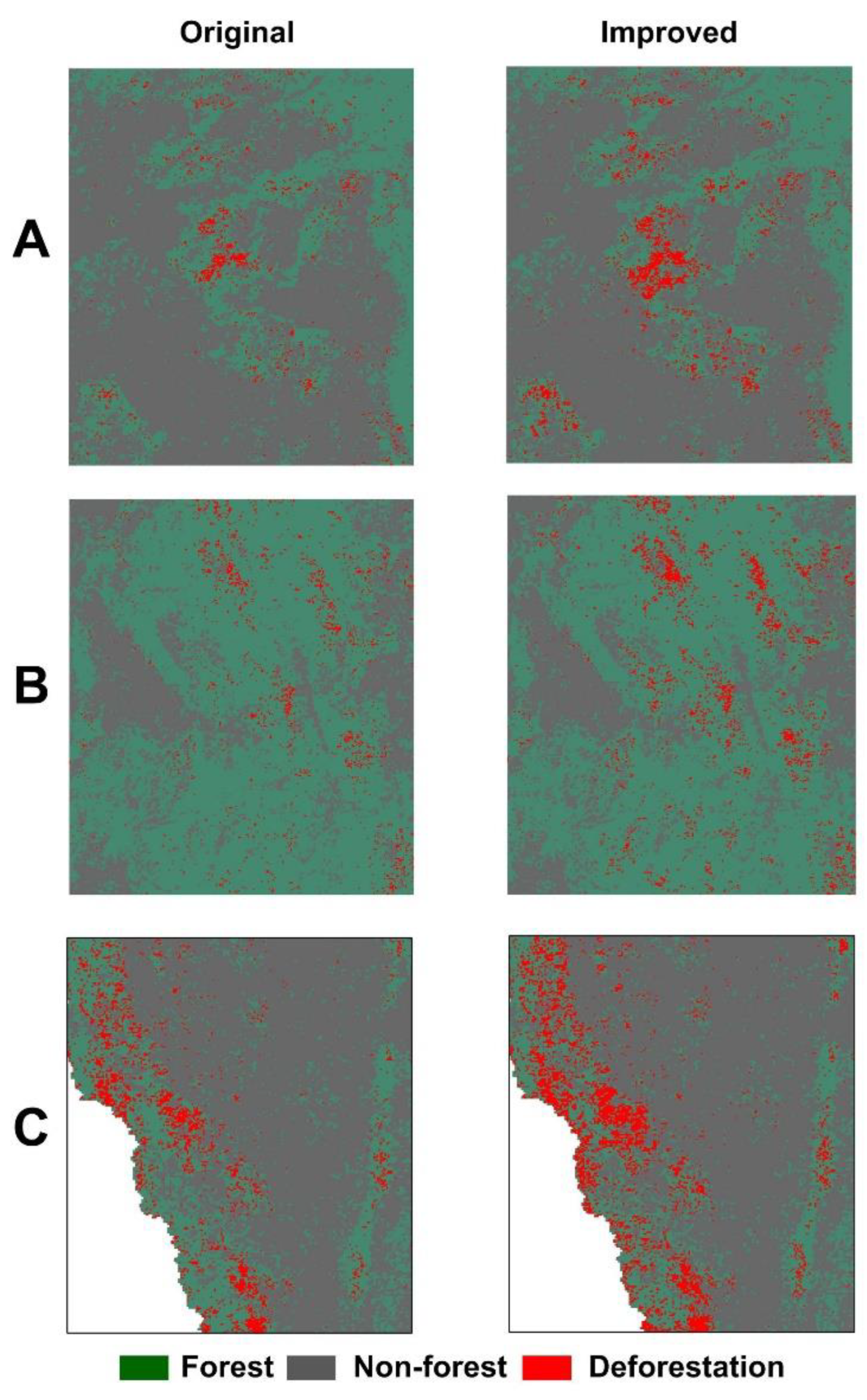
2.5. Highly Automated Vegetation Change Tracker

The description of VCT method can be explained as a physical interpretation for each pixel based on the enhanced IFZ. Therefore, the forest change should respond to the enhanced IFZ variation as the principle of IFZ is the measurement of likelihood for a pixel being a forest pixel. For persisting forest land, namely where no major disturbance has occurred during the years it was being monitored, the enhanced IFZ would remain low and relatively stable. For the whole study period, if a disturbance occurred, a sharp increase in the enhanced IFZ should be observed. In the same way, for the gradual regeneration process of a new forest stand after disturbance, a sequence of gradually decreasing IFZs will be detected. The conversion from non-forest land to forest land (i.e., forest restoration), or forest stand regeneration after disturbances that occurred before the first MODIS data collection were recorded, can be seen in the gradual decrease in the enhanced IFZ. In such a case, the IFZ would decrease from a high value to a level observed for undisturbed forests. One thing that should be noted is that as the regeneration of a forest usually takes at least several years for the regrowing trees to present a “forest appearance” in the spectral data, so the enhanced IFZ would reduce gradually rather than drop quickly from a high value to the level of close to 0. Finally, in general, the enhanced IFZ would remain high throughout the time series for persisting non-forest pixels that retained their non-forest character over the entire observation period. It is worth repeating that forest reconstruction is typically an extremely long process. Therefore, applying this understanding, the forest area in upland Myanmar was tracked during the first year of the observation period for pixels presenting forests.

The VCT method is based on the unique enhanced IFZ time profile of the aforementioned different land cover and forest change processes. Specific decision rules were used to identify the type of continuous land cover and to detect interference through a series of steps. First, pixel values that were always ~0 or very low throughout the observation period were distinguished as presenting “persisting forest”. Most forests with closed or near-close canopy cover should have values lower than the threshold of 3. In the meantime, due to SG filtering, the threshold was lower before processing. Based on the approximate probability interpretation of the enhanced IFZ, the threshold value was finally decided as 2.3. This threshold value was used to separate the low and high values throughout the implementation of the VCT method. Next, disturbance detection was applied to pixels not classified as “persisting forest”. Application of the VCT method enabled us to track the consecutive changes in the time series-enhanced IFZ for each pixel and record the years that exceeded the threshold, namely the years in which deforestation occurred.

3. Results

3.1. Accuracy Estimation

Google Earth was used to measure the number of ground truth pixels that were correctly classified. For this study, Google Earth images for the area of upland Myanmar were used for accuracy estimation. We generated a set of 300 random points and identified the corresponding points from the Google Earth image. The results showed that the total (overall) accuracy was 85.24%, and the Kappa (Κ) was 76.32%. Both values were acceptable. The coefficient K was rated as substantial; hence, the classified image was found to be suitable for further analysis. Moreover, the annual deforestation rate in our study was 0.79%, corresponding to the annual deforestation rate calculated by Wang (2016) (0.81%) for upland Myanmar [27].

Three samples were selected to measure the improvement. There was a clear difference between the original and improved VCT tracking results (Figure 2). Thirty-six percent (27% and 32%) of regions A (B and C) have different change detection results after applying improved time series IFZ. When using the filtered smoothed time series IFZ, there is more forest loss plotted on regions A, B, and C, and the result is more consistent with the annual deforestation rate calculated by Wang (2016) [27].

3.2. Spatio-Temporal Analysis to Assess Deforestation in the Study Area

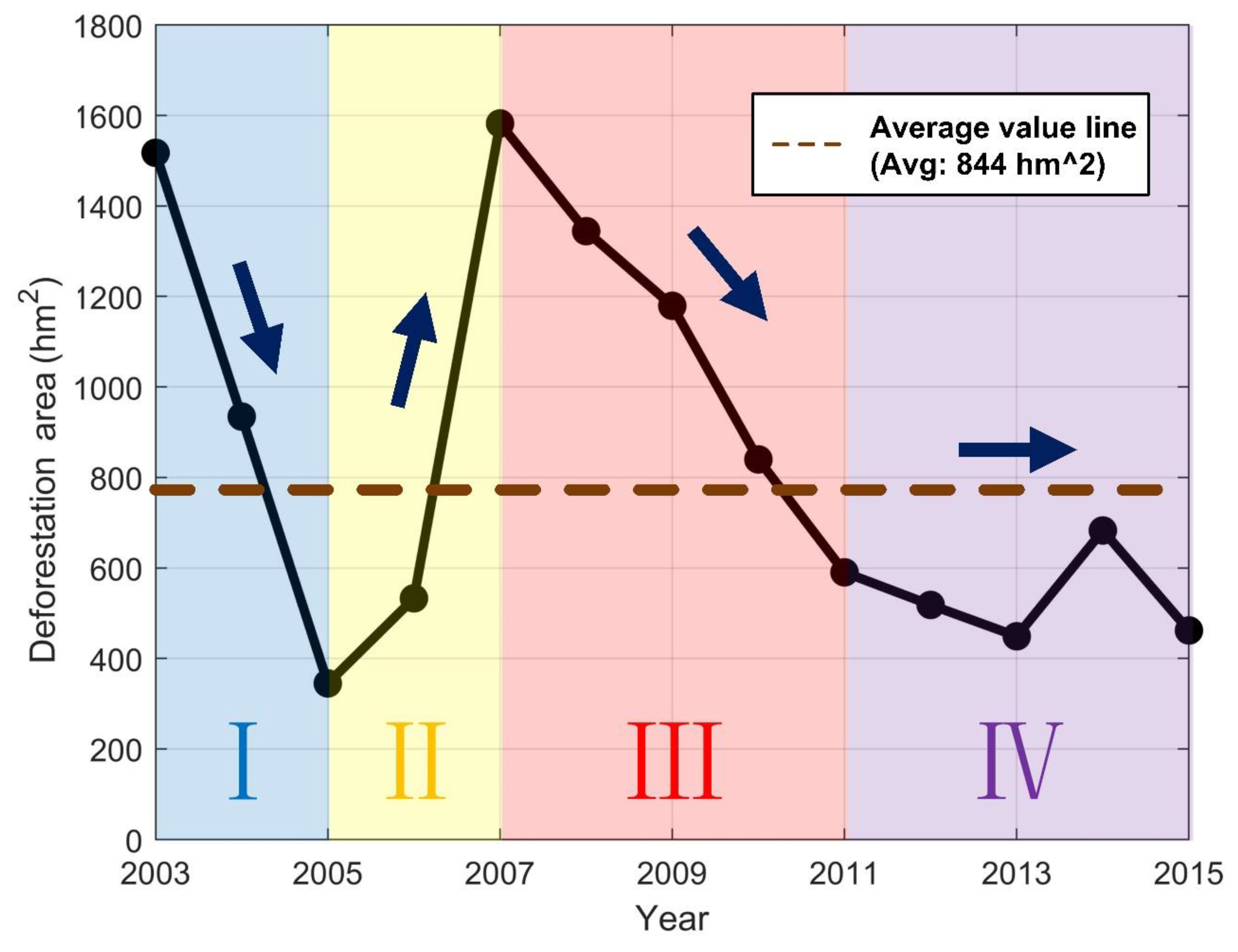
3.2.1. Temporal Change

Figure 3 shows the change in deforestation in upland Myanmar over the past 13–15 years. During this time, the annual deforestation area in Myanmar first decreased, then increased, decreased again, and finally stabilized. Based on the variation trend observed for the research period, the time can be divided into four stages. Stage I spans from 2003 to 2004, during which the annual deforestation area decreased from more than 1500 hm²/year to less than 400 hm²/year. Stage II lasted from 2005 to 2006, during which the annual deforestation area continued to grow, as did the year-by-year rate of increase until it reached the highest value in 2007, ~1580 hm² per year. The next stage, Stage III, started in 2007 and ended in 2010. The annual deforestation area decreased year by year during this stage. In Stage IV (2011–2015), the annual deforestation area fluctuated in the range of 400–700 hm²/year.

Compared with the average value line, in 2003 and 2007, the differences in the deforested area reached relatively high levels, reflecting more serious deforestation in those years. In 2005, the difference reached its maximum negative value, indicating that deforestation was relatively less extensive in that year. The difference was negative from 2010 to 2015, with specific year-to-year differences; in the last few years of the study period, the area of forest felled was relatively stable, and compared with the previous period, it was much less extensive.

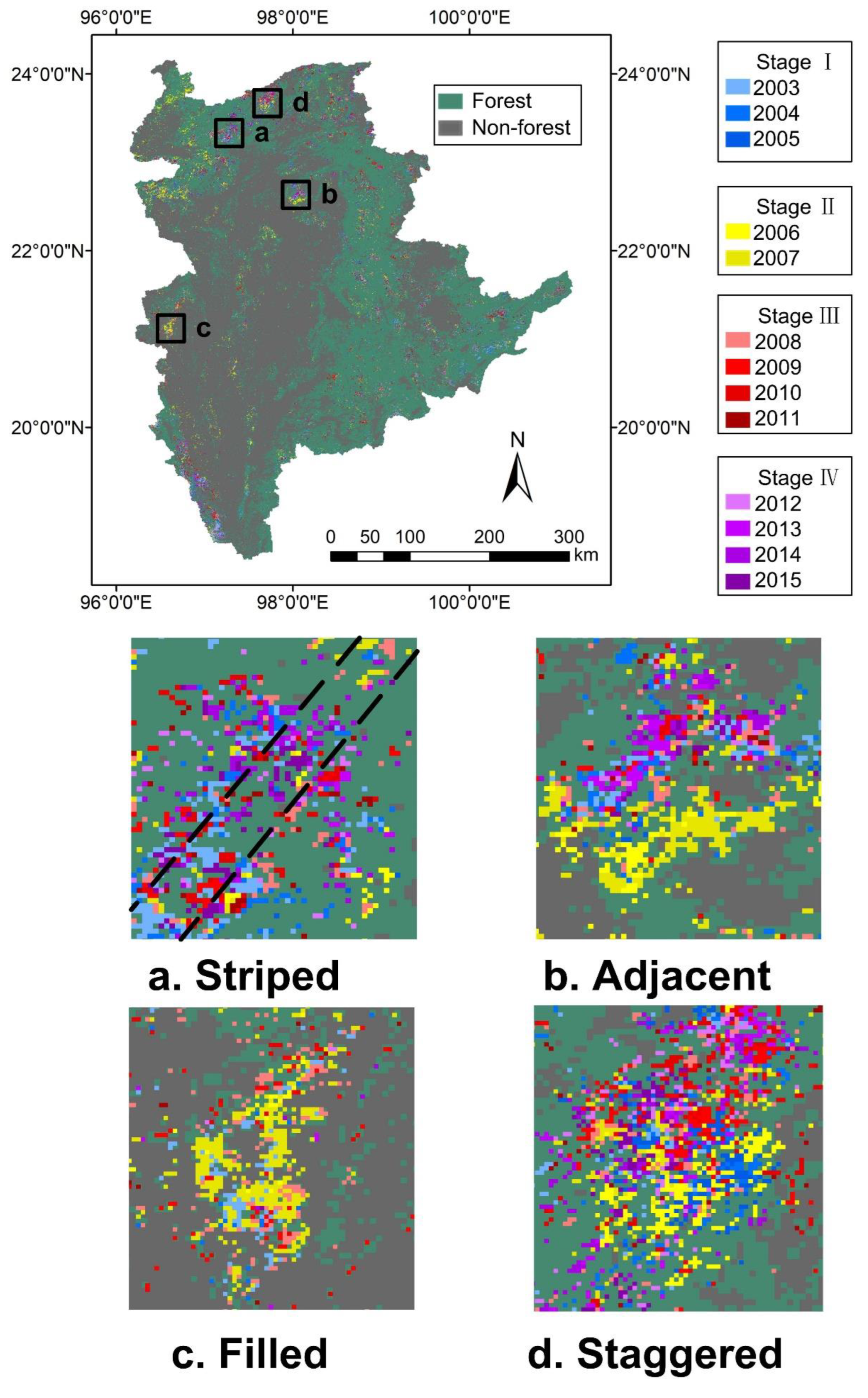
3.2.2. Spatial Distribution

Figure 4 shows the spatio-temporal information of deforestation pixels in upland Myanmar during the study period. Deforestation activities were typically concentrated locally, with large-scale centralized deforestation occurring at or near the edge of the forest. Among these activities, the large-scale deforestation that occurred during Stage I was mostly concentrated in the northern, southern, and southwestern parts of upland Myanmar. The concentrated deforestation areas of Stage II were generally concentrated in the northwest, center, and west, and a small and scattered deforestation area was distributed in the east. Deforestation activities were most widely distributed in this stage, and the deforestation area was also the largest. The concentrated deforestation areas of Stage III were distributed in the southeast, and small-scale deforestation was evident in the central and northern regions. The characteristics of this stage were mainly manifested as covering a wide distribution range and were small in scale. Stage IV was marked by large-scale deforestation activities in the northern and central parts of the study area. Moreover, small-scale deforestation was observed around the large-scale deforestation areas in the first three stages.

In terms of the mode of expansion, the deforestation features of the study area were categorized as “striped”, “adjacent”, “filled”, and “staggered”. The “striped” feature was characterized by a large time span, generally covering three or four stages. It specifically manifested as a band-like deforestation area at the edge of each originally deforested area. The “adjacent” mode of expansion was deciphered by the presence of two adjacent large-scale deforested areas. Different stages of centralized deforestation occurred in two adjacent forests, the time span covering two to three stages. The “filled” feature mainly referred to the “fill-in” deforestation that occurred in the original large-scale deforestation area. Most of such land marked the further expansion of the deforestation that occurred in the original forest area after large-scale deforestation. Lastly, the “staggered” expansion mode exemplified this complex multi-stage deforestation model. The deforestation area in this case showed disordered and small-scale deforestation in various stages. The time span of such deforestation typically covered three to four stages.

3.3. Elevation-Based Deforestation Dynamics

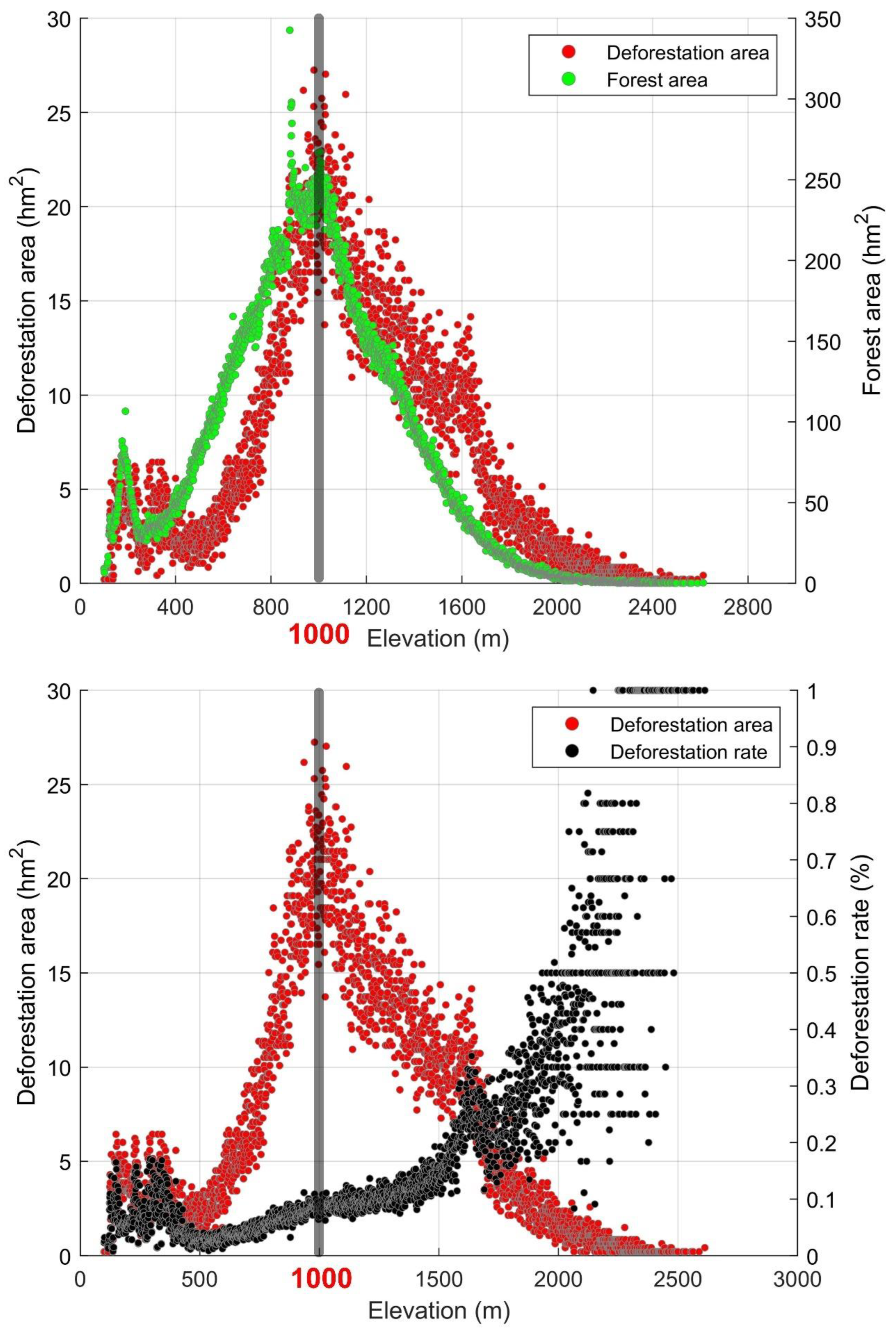
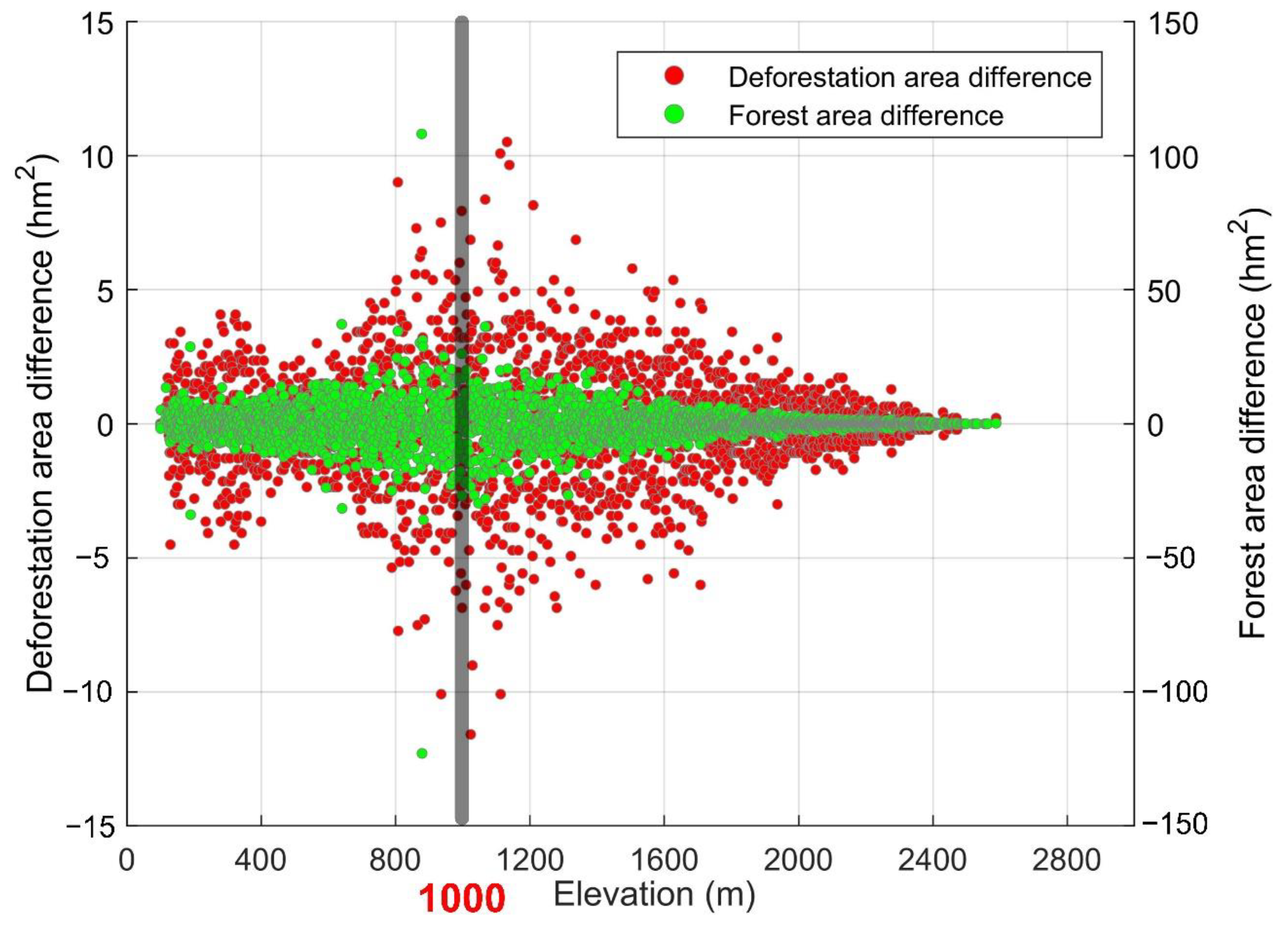
3.3.1. Elevation-Based Analysis for the Deforestation and Forest Areas

Figure 5 shows the changes in deforestation in upland Myanmar at various elevations during the study period. This result was compared with the elevation distributions of the forest area and the deforestation rate. The deforestation area was found to be positively correlated with the forest area over the change in elevation; that is, the larger the forest area, the larger the total deforestation area for a particular elevation. However, the deforestation rates at different elevations showed obvious differences in terms of segmentation characteristics: for hills below 500 m, the deforestation area and deforestation rate did not change significantly with height; for low mountains from elevations of 500 to 1000 m, the forest area, deforestation area, and deforestation rate were found to increase with elevation. The rate of deforestation increased, and the deforestation area reached its peak at an elevation of 1000 m. For plateaus over 1000 m, an increase in elevation was accompanied by a gradual decrease in the forest and deforestation areas. However, the deforestation rate continued to increase.

The deforestation area showed a general increasing trend followed by a decrease with elevation, and it reached its highest value at an elevation of ~1000 m. When the elevation exceeded 2000 m, the deforestation area reduced significantly. In the past, deforestation activities in this area were mainly concentrated in the mountainous region (elevation: ~1000 m), which has rich forest resources.

The forest area also showed an increase, followed by a decrease, with elevation. Its change trend mimicked that of the deforestation area as well, and the change in the deforestation area indicated a certain “lag”. Thus, the elevation distribution of the forest area affected the elevation distribution of the deforestation area. Moreover, forest endowment was the basis of the deforestation activities. Both the forest and deforestation areas peaked in plateau areas with elevations of ~1000 m, indicating that the abundant forest resources in this area were the primary reason for the large deforestation area. The deforestation rate showed a completely different trend from that observed for the change in the forest area: as the elevation increased, the deforestation rate continued to rise. Since the change trends for both the forest and deforestation areas were marked by an initial increase and then a decrease, the extents of the increase and decrease were essentially the same. The intensity of deforestation on the left- and right-hand sides of the 1000 m above sea level elevation was reflected in the deforestation rate, as it registered an increase. This result shows that although plateaus over 1000 m were not traditionally part of the main deforestation area due to the lack of forest resources in the past, they currently suffer a greater risk of deforestation.

Figure 5 shows that two main factors influenced the change in the deforestation area: the forest area owned and the elevation of that area. Clearly, at a certain elevation, the forest area was the decisive factor in determining the deforestation area, with the elevation of that area exerting a certain degree of impact as well. It is worth noting that although the degree and proportion of influence of the two above-stated factors differed, it was impossible to discern whether the difference in elevation also played a role. Therefore, we compared the relative differences in the forest and deforested areas by elevation which is shown in Figure 6. Furthermore, to eliminate the error caused by the possible difference in the elevation span, the value of the change in the deforestation area was divided by the elevation span between the two points. According to Figure 6, a strong correlation existed between the relative differences in the forest and deforestation areas, and the two values changed drastically at an elevation of ~1000 m. Therefore, the forest area was the main factor in determining the scale of deforestation. At an elevation of ~1000 m, the relative difference in the deforestation area varied much more than the corresponding value for the forest area. In other words, the deforestation area was greatly affected by the elevation at a height of ~1000 m during the study period.

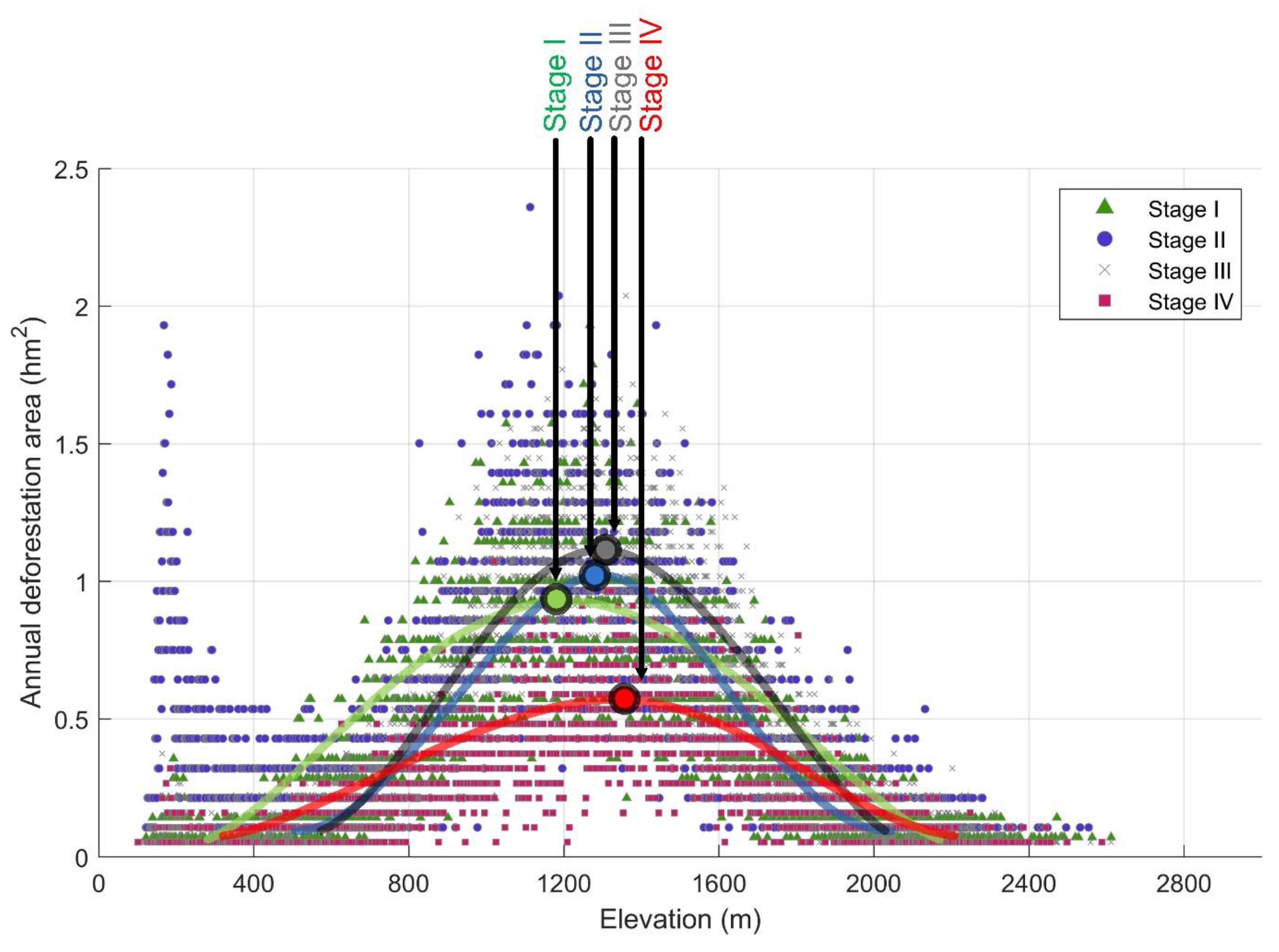
3.3.2. Elevation-Based Analysis for Deforestation Stages

To explore the changes in the elevation distribution of the deforestation area over time, we compared the elevation distribution scatter plots of the deforestation area in the four stages explained in Section 3.2.2. Figure 7 shows a scatter plot of the changes in the elevation of the deforestation area at different stages. The change trend of each stage in upland Myanmar first showed an increasing trend followed by a decreasing trend in Stages I and IV. The deforestation area was relatively low in these stages at elevations lower than 500 m. In Stages II and III, the deforestation area at elevations spanning from 0 to 500 m showed a negative correlation with elevation. Among them, the low-elevation deforestation area of Stage II was the highest, as was its decline, from ~4 to 1 hm². The low-elevation deforestation area of Stage III reduced from 2.5 to ~1 hm². The highest values in all four stages appeared between 1000 and 1500 m. Stages I, II, III, and IV reached their respective peaks at ~1200, 1250, 1300 m, and 1350 m, respectively. Thus, the elevation corresponding to the peak value in each stage gradually increased, proving that the center of deforestation shifted to high-elevation areas over time.

Comparing the distributions of the four stages in terms of area (Figure 7) showed the highest peak for the distribution corresponding to Stage III. In contrast, the distribution for Stage IV showed the lowest peak. Thus, we concluded that the change in the deforestation area first increased and then decreased, and that the scale of the deforestation activities in Stage IV was much smaller than those in the other stages.

3.3.3. The “Golden Cross” among the Elevation Segments

The previous results showed that the center of elevation for the deforestation area during the study period existed at an elevation of ~1000 m. Moreover, we observed that this center tended to shift gradually to higher elevations. To further study the time series dynamics of this migration, we used 500 m as the classification gradient to extract the time series changes in the deforestation area corresponding to each elevation segment. According to Figure 8, the deforestation area continued to remain low at elevations of 2000–2612 m, varying between ~20–50 hm². The deforestation areas at elevations of 80–500 m were comparatively higher in 2006 and 2007. The deforestation area for this elevation segment exceeded 200 hm² in 2007, while the corresponding values in the remaining years were equivalent to those at elevations of 2000–2612 m. Compared to the other segments, the deforestation area at 1000–1500 m was always the highest in each year. The time series deforestation area for this elevation segment reached its peak, ~750 hm², in 2007.

The changes in deforestation in the elevation segments of 500–1000 m and 1500–2000 m reflect the intensity of deforestation activities in the low- and high-elevation areas, respectively. This aspect can be corroborated by Figure 5; the richness of the forest resources at these two elevations was equivalent. Figure 8 shows that the deforestation area corresponding to the elevation segment of 500–1000 m before 2006 was higher than that for 1500–2000 m. The year 2007, the last year of Stage II, stands out for the “golden cross”, which can be observed in the temporal changes for these two elevation segments. After 2007, for each year under study, the deforestation area at 1500–2000 m always exceeded that at 500–1000 m, indicating that after 2007, the deforestation activities in high-elevation areas began to intensify. The intersection of the two line graphs in question (Figure 8) shows that the shift of the center of elevation of deforestation to the higher-elevation segment occurred in 2007, and there was no sign of a fall thereafter.

4. Discussion

4.1. High Applicability of the Enhanced Integrated Forest Score and Vegetation Change Tracker for REDD+ MRV

The main driver of deforestation in upland Myanmar is the expansion of shifting cultivation, the mitigation of which requires timely monitoring and evaluation of local forest conditions. However, forest monitoring in this region presents some problems. First, the obtained experimental data contain noise due to atmospheric interference. This noise greatly interferes with the accuracy of forest monitoring results. Second, in large-area forests, such as the study region, forest monitoring and assessment require real-time dynamic analyses, which demand high efficiency and automation. Improvement in these aspects will help the timely adaptation to different local forest change models and information updates on forest changes, thereby ensuring the implementation of REDD+ policies.

This study used a forest dynamic monitoring method called VCT for timely monitoring and evaluation of local forest conditions. The intention here was to analyze annual time series deforestation in the study area, upland Myanmar, using enhanced IFZ data, and to visualize the results spatially using the coordinates of each point. This algorithm is based on the spectral-temporal properties of forest areas as well as the disturbance and post-disturbance recovery activities. Firstly, our algorithm analyzed each pixel of the individual image to extract indicators for measuring the likelihood to forest based on the classification by pre-generated forest mask. Then, it simultaneously analyzed all the images within an enhanced IFZ to detect disturbances and used a tracker to obtain information of post-disturbance activities after each disturbance. Visual assessment of the products from the disturbance year revealed that the majority of them were reasonably reliable.

Overall, the smoothness of the enhanced IFZ was greatly improved. Simultaneously, because the time information of the IFZ change was retained, the results of the application of the enhanced IFZ to the VCT method were enhanced. The IFZ is very sensitive to disturbances caused by clouds or the atmosphere, and it may experience sudden rises and drops within a short time period [65,66]. The enhanced IFZ, in contrast, reduced the interference of noise and could handle certain levels of bad observations in the time series IFZ, such that they had minimum or no impact on the derived disturbance products. Thus, when using the VCT method, the enhanced IFZ gradually reduced the step of noise identification, thus improving the operating efficiency. In addition, the enhanced IFZ did not change on the time axis, even as it adhered to the overall change law of the IFZ to the extent possible. These aspects improved the accuracy of the VCT results by a certain degree.

The MRV framework refers to the processes of carbon emission quantification and data quality assurance, including MRV [70]. It should be noted that the monitoring method, which is part of the REDD+ MRV system, needs to be improved in terms of accuracy when deployed for rapid identification purposes in large-area forests. Our study capitalized on the strengths of high-automation-based forest dynamic monitoring, which can efficiently record real-time changes in forests. The proposed REDD+ MRV complementary system was found to be able to enhance the information content and accuracy of change reporting, reduce costs considerably, assess the efficacy of spatio-temporal forest dynamics, and extend the spatial framework to couple local and national monitoring systems [71]. From this viewpoint, the study adds novelty to the literature in terms of widening the application base of the evolving REDD+ MRV system and drawing the attention of policymakers for its appropriate uptake.

4.2. Shifting of the Center of Elevation of the Deforestation Area

The distribution of the deforestation area in terms of elevation was mainly affected by two factors. This influence also determined the distribution and probable trends of deforestation across different elevation segments. The distribution characteristics of the deforestation at different elevations in this study were based on the evaluation of the destruction of forest resources in upland Myanmar across these elevation segments. Our research indicated that the center of elevation of the deforestation area was ~1000 m above sea level, and a potential risk of deforestation was identified at high elevations as well. Regarding the reason behind this trend, first, the elevation distribution range is dependent on human activities, a factor that continues be dynamic. Given the rapid population growth in upland Myanmar and technological improvements such as large-scale machinery applications, the range of human activities across elevations will likely continue to expand, either passively or actively. Second, the distribution of the deforestation area depends on local forest endowment; in other words, the distribution of forests across elevation segments affects the characteristics of the distribution of deforestation by elevation. In addition to the distribution of the forest by elevation, the secondary forest that generates after the farmland is left idle due to shifting cultivation, and this is an important factor affecting the recurrence of deforestation [72]. The distribution characteristics of deforestation at different elevations in this study were based on the evaluation of forest resource destruction in upland Myanmar across different ~500-m elevation segments. The division of farmland in the study area and its elevation are also important factors in this regard. Previous studies have shown that there is a potential risk of deforestation at high elevations and that shifting agriculture, which is traditionally implemented in Myanmar’s farmlands, accounts for more than 80% of the total farmland area. The main characteristics of this farming method include the selection of older trees for cutting and burning, increasing the fertility of farmland, as well as the selection of areas with sufficient light [32]. These demands are better satisfied in high-elevation areas, where sunlight is supplied throughout the year and the forest cover tends to be older [73]. Thus, the trend of deforestation in upland Myanmar will likely shift to the high-elevation forests in the future.

4.3. Human-Driven Deforestation Patterns

As shown in Figure 4, the “striped” pattern is characterized by a large formation time span, and the adjacent strips correspond to consecutive deforestation years. This pattern of deforestation is the result of small-scale deforestation activities taking place on the boundaries of large-scale deforestation areas, and the fellers tend to belong to the same village or group of developers [74]. The striped deforestation model reflects the expansion method of shifting cultivation, that is, the continuous expansion of existing agricultural land. In recent years, some scholars have pointed out that should the frequency of this deforestation pattern increase, it is most likely attributable to the population expansion of local villages and the rapid development of native industries.

The adjacent spatial characteristics are typically manifested as two or more large-scale deforestation events that occur in adjacent forest areas at different times. This adjacency is caused by either the development of the same village or village development in general. Both causes involve the migration of villagers. This is typically due to the loss of fertility of the previously deforested area and the influence of topography; it is impossible to implement the “striped” mode of deforestation expansion. Moreover, the villagers would hold on to their agricultural lands at all costs [75]. In addition, of note is the fact that it is not possible to identify from the spatial pattern diagram which of these two causes are responsible for the current state of affairs in the study area.

The “filled” pattern refers to a common deforestation mode, mainly secondary deforestation, based on a certain scale of the deforestation area. This pattern can be regarded as an extension of the “adjacent” pattern. The time span of this deforestation model generally spans three to four stages, because the filled areas are typically used as agricultural land for long-term cultivation. Moreover, because the “filled” pattern itself is a follow-up development model of deforestation activities at a certain scale, theoretically, a certain degree of secondary deforestation has occurred in most areas of upland Myanmar [75]. This pattern was also the most common deforestation development model in this region.

“Staggered” deforestation is a complicated phenomenon. This deforestation pattern depends on the terrain and the factors that cause the deforestation. Staggered areas occur in plains or plateau areas with suitable terrain as well as large forest areas. This pattern tends to be accompanied by small-scale or individual deforestation behavior, and multiple parties are involved. Thus, the spatial deforestation pattern in this case appears to be chaotic over time. This pattern of deforestation can be compared to “cannibalization”. The time span of occurrence generally spans three to four stages, and its scale depends on the number of groups that cause the deforestation.

4.4. The “Golden Cross” Due to Exacerbation of Human Activity

Figure 4 showed that the change in the center of elevation of the deforestation area generally tended to increase first and then decrease, reaching the highest value at an elevation of ~1000 m. Figure 6 compared the time series changes of the deforestation area over ~500-m elevation gradients. Therefore, the deforestation area in each year on the time series of the curve with an elevation of 500–1000 m and a curve with an elevation of 1500–2000 m were relatively low. As mentioned earlier, the deforestation area at the elevation of ~1000 m increased year by year. However, as the government has enforced stricter control over forest areas at this elevation, the center of elevation of the deforestation shifted over time. After analyzing the data from one year to the next and reviewing the changes in deforestation comprehensively, we showed that the center of elevation of the deforestation area presented a rising trend. This conclusion was also corroborated by Figure 6; for all the years under study, the areas of deforestation at elevations of 1000–1500 m were relatively high. Comparing the changes in the time series of the deforestation area at elevations of 500–1000 and 1500–2000 m improved our understanding of the migration of the center of elevation of deforestation. If the former is high, then the center of elevation of the deforestation area tends to be low, and vice versa. As shown in Figure 7, in 2007, the corresponding line graphs crossed, and the deforestation area corresponding to the latter has remained relatively high since then.

We introduced the concept of the “golden cross” to describe this change. It can be seen that the cross occurred in 2007, and only one cross occurred during the study period. After this crossing, the line graph corresponding to the elevation segment of 1500–2000 m has always remained above that of the 500–1000 m segment. Therefore, we proposed that before 2007, deforestation was more serious in low- and high-elevation areas. Between 2007 and 2015, deforestation shifted to high-elevation areas. Thus, the point of crossing reflects the turning point of the changes in deforestation. Consequently, we focused on the deforestation in 2007 to analyze the subsequent shift of its center of elevation.

5. Conclusions

This research focused on the deforestation caused by the expansion of shifting cultivation in upland Myanmar between 2003 and 2015. We analyzed the spatial pattern of deforestation and its distribution based on elevation. MODIS data were used to extract forest information and generate an enhanced IFZ based on SG filtering. This score was then applied to the VCT method. Deforestation analysis based on elevation was performed using the results of the VCT approach. We extracted four spatial deforestation models for upland Myanmar and determined that the center of elevation of the deforestation existed at ~1000 m. We also determined the occurrence and significance of the “golden cross” in 2007, illustrating that the center of elevation of the deforestation shifted to a higher elevation thereafter.

Spatially, the expansion of shifting cultivation in upland Myanmar showed different patterns due to the influence of forest endowments, topography, and human activities. As the forest resources at the elevation of 1000 m were relatively rich, driving intense human activities, the area corresponding to this elevation became the center of deforestation. Moreover, the extensive coverage by primary forests in high-elevation areas and technological developments caused the center of elevation of the deforestation to shift to high-elevation areas. Accurate estimation of the expansion of shifting cultivation may be essential for calculating realistic future land use scenarios.

Our research also highlighted that specific forest areas with real-time dynamic changes, such as those in upland Myanmar, can be better assessed through the enhanced IFZ. Our research applied the VCT method with enhanced IFZ analysis and proved its higher accuracy. We believe that these results are of great significance for the implementation of the REDD+ MRV framework.

References

1. Walker, X.J.; Rogers, B.M.; Veraverbeke, S.; Johnstone, J.F.; Baltzer, J.L.; Barrett, K.; Bourgeau-Chavez, L.; Day, N.J.; de Groot, W.J.; Dieleman, C.M.; et al. Fuel availability not fire weather controls boreal wildfire severity and carbon emissions. Nat. Clim. Chang. 2020, 10, 1130–1136. [Google Scholar] [CrossRef]
2. Wang, Y.; Wang, Z.; Zameer, H. Structural characteristics and evolution of the “international trade-carbon emissions” network in equipment manufacturing industry: International evidence in the perspective of global value chains. Environ. Sci. Pollut. Res. Lnt. 2021, 28, 25886–25905. [Google Scholar] [CrossRef] [PubMed]
3. Ngo, D.T.; Le, A.V.; Le, H.T.; Stas, S.M.; Le, T.C.; Tran, H.D.; Pham, T.; Le, T.T.; Spracklen, B.D.; Langan, C.; et al. The potential for REDD+ to reduce forest degradation in Vietnam. Environ. Res. Lett. 2020, 15, 074025. [Google Scholar] [CrossRef]
4. Villa, P.M.; Martins, S.V.; de Oliveira Neto, S.N.; Rodrigues, A.C.; Hernández, E.P.; Kim, D.G. Policy forum: Shifting cultivation and agroforestry in the Amazon: Premises for REDD+. For. Policy Econ. 2020, 118, 102217. [Google Scholar] [CrossRef]
5. Csillik, O.; Kumar, P.; Asner, G.P. Challenges in estimating tropical forest canopy height from planet dove imagery. Remote Sens. 2020, 12, 1160. [Google Scholar] [CrossRef] [Green Version]
6. Silva, J.M.N.; Carreiras, J.M.B.; Rosa, I.; Pereira, J.M.C. Greenhouse gas emissions from shifting cultivation in the tropics, including uncertainty and sensitivity analysis. J. Geophys. Res. Atmos. 2011, 116, D20304. [Google Scholar] [CrossRef] [Green Version]
7. Corbera, E.; Schroeder, H. Governing and implementing REDD+. Environ. Sci. Policy 2011, 14, 89–99. [Google Scholar] [CrossRef]
8. Hargita, Y.; Günter, S.; Köthke, M. Brazil submitted the first REDD+ reference level to the UNFCCC—Implications regarding climate effectiveness and cost-efficiency. Land Use Policy 2016, 55, 340–347. [Google Scholar] [CrossRef]
9. Andoh, J.; Lee, Y. National REDD+ strategy for climate change mitigation: A review and comparison of developing countries. Sustainability 2018, 10, 4781. [Google Scholar] [CrossRef] [Green Version]
10. Sandker, M.; Carrillo, O.; Leng, C.; Lee, D.; d’Annunzio, R.; Fox, J. The Importance of High–Quality Data for REDD+ Monitoring and Reporting. Forests 2021, 12, 99. [Google Scholar] [CrossRef]
11. Pham, T.T.; Moeliono, M.; Yuwono, J.; Dwisatrio, B.; Gallo, P. REDD+ finance in Brazil, Indonesia, and Vietnam: Stakeholder perspectives between 2009-2019. Glob. Environ. Chang. 2021, 70, 102330. [Google Scholar] [CrossRef]
12. Luttrell, C.; Loft, L.; Gebara, M.F.; Kweka, D.; Brockhaus, M.; Angelsen, A.; Sunderlin, W.D. Who should benefit from REDD+? Rationales and realities. Ecol. Soc. 2013, 18, 52. [Google Scholar] [CrossRef] [Green Version]
13. Hoang, M.H.; Do, T.H.; Pham, M.T.; Van Noordwijk, M.; Minang, P.A. Benefit distribution across scales to reduce emissions from deforestation and forest degradation (REDD+) in Vietnam. Land Use Policy 2013, 31, 48–60. [Google Scholar] [CrossRef]
14. Karsenty, A.; Vogel, A.; Castell, F. Carbon rights, REDD+ and payments for environmental services. Environ. Sci. Policy 2014, 35, 20–29. [Google Scholar] [CrossRef]
15. Nyamari, N.; Cabral, P. Impact of land cover changes on carbon stock trends in Kenya for spatial implementation of REDD+ policy. Appl. Geogr. 2021, 133, 102479. [Google Scholar] [CrossRef]
16. Cappello, C.; Pratihast, A.K.; Pérez Ojeda del Arco, A.; Reiche, J.; De Sy, V.; Herold, M.; Vivanco Vicencio, R.E.; Castillo Soto, D. Alert-Driven Community-Based Forest Monitoring: A Case of the Peruvian Amazon. Remote Sens. 2022, 14, 4284. [Google Scholar] [CrossRef]
17. Aryal, R.R.; Wespestad, C.; Kennedy, R.; Dilger, J.; Dyson, K.; Bullock, E.; Khanal, N.; Kono, M.; Poortinga, A.; Saah, D.; et al. Lessons Learned While Implementing a Time-Series Approach to Forest Canopy Disturbance Detection in Nepal. Remote Sens. 2021, 13, 2666. [Google Scholar] [CrossRef]
18. Fry, B.P. Community forest monitoring in REDD+: The ‘M’in MRV? Environ. Sci. Policy 2011, 14, 181–187. [Google Scholar]
19. Tun, Z.N.; Dargusch, P.; McMoran, D.J.; McAlpine, C.; Hill, G. Patterns and Drivers of Deforestation and Forest Degradation in Myanmar. Sustainability 2021, 13, 7539. [Google Scholar]
20. Herold, M.; Skutsch, M.M. Measurement, reporting and verification for REDD+: Objectives, capacities and institutions. In Realising REDD+: National Strategy and Policy Options; Angelsen, A., Brockhaus, M., Eds.; Center for International Forestry Research: Bogor, Indonesia, 2009; pp. 84–100. ISBN 978-6-02-869303-5. [Google Scholar]
21. Goslee, K.M.; Pearson, T.R.; Bernal, B.; Simon, S.L.; Sukhdeo, H. Comprehensive Accounting for REDD+ Programs: A Pragmatic Approach as Exemplified in Guyana. Forests 2020, 11, 1265. [Google Scholar] [CrossRef]
22. Biswas, S.; Huang, Q.; Anand, A.; Mon, M.S.; Arnold, F.E.; Leimgruber, P. A multi sensor approach to forest type mapping for advancing monitoring of sustainable development goals (SDG) in Myanmar. Remote Sens. 2020, 12, 3220. [Google Scholar] [CrossRef]
23. Soe, K.T.; Yeo-Chang, Y.O.U.N. Perceptions of forest-dependent communities toward participation in forest conservation: A case study in Bago Yoma, South-Central Myanmar. Forest Policy Econ. 2019, 100, 129–141. [Google Scholar] [CrossRef]
24. Michinaka, T.; Hlaing, E.E.S.; Oo, T.N.; Mon, M.S.; Sato, T. Forecasting forest areas in Myanmar based on socioeconomic factors. Forests 2020, 11, 100. [Google Scholar] [CrossRef] [Green Version]
25. Reddy, C.S.; Pasha, S.V.; Satish, K.V.; Unnikrishnan, A.; Chavan, S.B.; Jha, C.S.; Diwakar, P.G.; Dadhwal, V.K. Quantifying and predicting multi-decadal forest cover changes in Myanmar: A biodiversity hotspot under threat. Biodivers. Conserv. 2019, 28, 1129–1149. [Google Scholar] [CrossRef]
26. Schmid, M.; Heinimann, A.; Zaehringer, J.G. Patterns of land system change in a Southeast Asian biodiversity hotspot. Appl. Geogr. 2021, 126, 102380. [Google Scholar] [CrossRef]
27. Wang, C.; Myint, S.W. Environmental concerns of deforestation in Myanmar 2001–2010. Remote Sens. 2016, 8, 728. [Google Scholar] [CrossRef] [Green Version]
28. Shimizu, K.; Ota, T.; Mizoue, N.; Yoshida, S. Patch-Based Assessments of Shifting Cultivation Detected by Landsat Time Series Images in Myanmar. Sustainability 2018, 10, 3350. [Google Scholar] [CrossRef] [Green Version]
29. Swe, K.N.; Nawata, E. Changing Practices from Swidden to Permanent Agriculture in Traditional Swidden Cultivation Areas-Case Studies in Three Karen Villages of the Bago Mountains, Myanmar. Trop. Agric. Develop. 2020, 64, 80–89. [Google Scholar]
30. Fukushima, M.; Kanzaki, M.; Thein, H.M. Recovery process of fallow vegetation in the traditional Karen swidden cultivation system in the Bago mountain range, Myanmar. Southeast Asian Stud. 2007, 45, 317–333. [Google Scholar]
31. Angelsen, A. Shifting cultivation and “deforestation”: A study from Indonesia. World Dev. 1995, 23, 1713–1729. [Google Scholar] [CrossRef]
32. Paul, S.; Das, T.K.; Pharung, R.; Ray, S.; Mridha, N.; Kalita, N.; Ralte, V.; Borthakur, S.; Burman, R.R.; Tripathi, A.K.; et al. Development of an indicator based composite measure to assess livelihood sustainability of shifting cultivation dependent ethnic minorities in the disadvantageous Northeastern region of India. Ecol. Indic. 2020, 110, 105934. [Google Scholar] [CrossRef]
33. Thong, P.; Sahoo, U.K.; Thangjam, U.; Pebam, R. Pattern of forest recovery and carbon stock following shifting cultivation in Manipur, North-East India. PLoS ONE 2020, 15, e0239906. [Google Scholar] [CrossRef] [PubMed]
34. Heinimann, A.; Mertz, O.; Frolking, S.; Egelund Christensen, A.; Hurni, K.; Sedano, F.; Parsons Chini, L.; Sahajpal, R.; Hansen, M.; Hurtt, G. A global view of shifting cultivation: Recent, current, and future extent. PLoS ONE 2017, 12, e0184479. [Google Scholar] [CrossRef] [Green Version]
35. Molinario, G.; Hansen, M.C.; Potapov, P.V. Forest cover dynamics of shifting cultivation in the Democratic Republic of Congo: A remote sensing-based assessment for 2000–2010. Environ. Res. Lett. 2015, 10, 094009. [Google Scholar] [CrossRef]
36. Thet, A.P.P.; Tokuchi, N. Traditional knowledge on shifting cultivation of local communities in Bago Mountains, Myanmar. J. For. Res. 2020, 25, 347–353. [Google Scholar] [CrossRef]
37. Lu, S.; Zhang, C.; Lu, H. Spatio-temporal dynamics of shifting cultivation in Upland Myanmar using time series images and implications for REDD+. In Land Surface and Cryosphere Remote Sensing IV, Proceedings of International Society for Optics and Photonics, Honolulu, HI, USA, 25–26 September 2018; SPIE: Bellingham, WA, USA, 2018; Volume 10777, p. 107770O. [Google Scholar]
38. Zwartendijk, B.W.; Van Meerveld, H.J.; Ghimire, C.P.; Bruijnzeel, L.A.; Ravelona, M.; Jones, J.P.G. Rebuilding soil hydrological functioning after swidden agriculture in eastern Madagascar. Agric. Ecosyst. Environ. 2017, 239, 101–111. [Google Scholar] [CrossRef] [Green Version]
39. Das, P.; Mudi, S.; Behera, M.D.; Barik, S.K.; Mishra, D.R.; Roy, P.S. Automated Mapping for Long-Term Analysis of Shifting Cultivation in Northeast India. Remote Sens. 2021, 13, 1066. [Google Scholar] [CrossRef]
40. Mon, M.S.; Mizoue, N.; Htun, N.Z.; Kajisa, T.; Yoshida, S. Factors affecting deforestation and forest degradation in selectively logged production forest: A case study in Myanmar. For. Ecol. Manag. 2012, 267, 190–198. [Google Scholar] [CrossRef]
41. D’Arrigo, R.; Palmer, J.; Ummenhofer, C.C.; Kyaw, N.N.; Krusic, P. Three centuries of Myanmar monsoon climate variability inferred from teak tree rings. Geophys. Res. Lett. 2011, 38, L24705. [Google Scholar] [CrossRef] [Green Version]
42. Zeng, Z.; Wang, D.; Yang, L.; Wu, J.; Ziegler, A.D.; Liu, M.; Ciais, P.; Searchinger, T.D.; Yang, Z.L.; Chen, D.; et al. Deforestation-induced warming over tropical mountain regions regulated by elevation. Nat. Geosci. 2021, 14, 23–29. [Google Scholar] [CrossRef]
43. Rudel, T.K. Changing agents of deforestation: From state-initiated to enterprise driven processes, 1970–2000. Land Use Policy 2007, 24, 35–41. [Google Scholar] [CrossRef]
44. Trujillo, E.; Molotch, N.P.; Goulden, M.L.; Kelly, A.E.; Bales, R.C. Elevation-dependent influence of snow accumulation on forest greening. Nat. Geosci. 2012, 5, 705–709. [Google Scholar] [CrossRef]
45. Slot, M.; Cala, D.; Aranda, J.; Virgo, A.; Michaletz, S.T.; Winter, K. Leaf heat tolerance of 147 tropical forest species varies with elevation and leaf functional traits, but not with phylogeny. Plant Cell Environ. 2021, 44, 2414–2427. [Google Scholar] [CrossRef] [PubMed]
46. Han, J.C.; Huang, Y.; Zhang, H.; Wu, X. Characterization of elevation and land cover dependent trends of NDVI variations in the Hexi region, northwest China. J. Environ. Manag. 2019, 232, 1037–1048. [Google Scholar] [CrossRef]
47. Fyllas, N.M.; Bentley, L.P.; Shenkin, A.; Asner, G.P.; Atkin, O.K.; Díaz, S.; Enquist, B.J.; Farfan-Rios, W.; Gloor, E.; Guerrieri, R.; et al. Solar radiation and functional traits explain the decline of forest primary productivity along a tropical elevation gradient. Ecol. Lett. 2017, 20, 730–740. [Google Scholar] [CrossRef]
48. Murray, N.J.; Keith, D.A.; Tizard, R.; Duncan, A.; Htut, W.T.; Hlaing, N.; Oo, A.H.; Ya, K.Z.; Grantham, H. Threatened Ecosystems of Myanmar. An IUCN Red List of Ecosystems Assessment, 1st ed.; Wildlife Conservation Society: Randwick, Australia, 2020; ISBN 978-0-9903852-5-7. [Google Scholar]
49. Wang, Y.; Ziv, G.; Adami, M.; de Almeida, C.A.; Antunes, J.F.G.; Coutinho, A.C.; Esquerdo, J.C.D.M.; Gomes, A.R.; Galbraith, D. Upturn in secondary forest clearing buffers primary forest loss in the Brazilian Amazon. Nat. Sustain. 2020, 3, 290–295. [Google Scholar] [CrossRef]
50. Bisi, F.; Gagliardi, A.; Cremonesi, G.; Colombo, R.; Mazzamuto, M.V.; Wauters, L.A.; Preatoni, D.G.; Martinoli, A. Distribution of wildlife and illegal human activities in the Lampi marine National Park (Myanmar). Environ. Conserv. 2019, 46, 163–170. [Google Scholar] [CrossRef] [Green Version]
51. Kmoch, L.; Palm, M.; Persson, U.M.; Jepsen, M.R. Access mapping highlights risks from land reform in upland Myanmar. J. Land Use Sci. 2021, 16, 34–54. [Google Scholar] [CrossRef]
52. Kmoch, L.; Palm, M.; Persson, U.M.; Rudbeck Jepsen, M. Upland livelihoods between local land and global labour market dependencies: Evidence from Northern Chin State, Myanmar. Sustainability 2018, 10, 3707. [Google Scholar] [CrossRef] [Green Version]
53. Aung, A.K. The primate-bearing Pondaung Formation in the upland area, northwest of central Myanmar. In Anthropoid Origins; Springer: Boston, MA, USA, 2004; pp. 205–217. [Google Scholar]
54. Borras, S.M., Jr.; Franco, J.C.; Nam, Z. Climate change and land: Insights from Myanmar. World Dev. 2020, 129, 104864. [Google Scholar] [CrossRef]
55. D’Arrigo, R.; Ummenhofer, C.C. The climate of Myanmar: Evidence for effects of the Pacific Decadal Oscillation. Int. J. Climatol. 2015, 35, 634–640. [Google Scholar] [CrossRef] [Green Version]
56. Sein, K.K.; Chidthaisong, A.; Oo, K.L. Observed trends and changes in temperature and precipitation extreme indices over Myanmar. Atmosphere 2018, 9, 477. [Google Scholar] [CrossRef] [Green Version]
57. Rao, M.; Htun, S.; Platt, S.G.; Tizard, R.; Poole, C.; Myint, T.; Watson, J.E. Biodiversity conservation in a changing climate: A review of threats and implications for conservation planning in Myanmar. Ambio 2013, 42, 789–804. [Google Scholar] [CrossRef] [PubMed] [Green Version]
58. Htun, N.Z. Biodiversity in Myanmar. In Global Biodiversity, 1st ed.; Apple Academic Press: Palm Bay, FL, USA, 2018; pp. 753–815. ISBN 9780429487743. [Google Scholar]
59. Yang, R.; Luo, Y.; Yang, K.; Hong, L.; Zhou, X. Analysis of forest deforestation and its driving factors in Myanmar from 1988 to 2017. Sustainability 2019, 11, 3047. [Google Scholar] [CrossRef]
60. Lim, C.L.; Prescott, G.W.; De Alban, J.D.T.; Ziegler, A.D.; Webb, E.L. Untangling the proximate causes and underlying drivers of deforestation and forest degradation in Myanmar. Conserv. Biol. 2017, 31, 1362–1372. [Google Scholar] [CrossRef] [PubMed] [Green Version]
61. Li, Y.; Andrés, V.; Yang, W.; Chen, X.D.; Zhang, J.D.; Ouyang, Z.Y. Effects of conservation policies on forest cover change in giant panda habitat regions, China. Land Use Policy 2013, 33, 42–53. [Google Scholar] [CrossRef] [Green Version]
62. Dong, J.; Xiao, X.; Sheldon, S.; Biradar, C.; Duong, N.D.; Hazarika, M. A comparison of forest cover maps in Mainland Southeast Asia from multiple sources: PALSAR, MERIS, MODIS and FRA. Remote Sens. Environ. 2012, 127, 60–73. [Google Scholar] [CrossRef]
63. Dou, X.F.; Jiapa, A.; Li, Y.H.; Guan, Z.Z.; Wang, X.M.; Lv, Y.N.; Tian, L.L.; Li, X.; Zhang, X.C.; Sun, Y.L.; et al. Remote sensing of land coverage and investigation of plague risk among small mammals in Beijing, China. Chin. J. Vector Biol. Control 2013, 24, 43–46. [Google Scholar]
64. Yan, X.U.; Zhang, J. Detecting major phenological stages of rice using MODIS-EVI data and Symlet11 wavelet in Northeast China. Acta Ecol. Sin. 2012, 7, 1–4. [Google Scholar]
65. Huang, C.; Goward, S.N.; Masek, J.G.; Thomas, N.; Zhu, Z.; Vogelmann, J.E. An automated approach for reconstructing recent forest disturbance history using dense Landsat time series stacks. Remote Sens. Environ. 2010, 114, 183–198. [Google Scholar] [CrossRef]
66. Huang, C.; Ling, P.Y.; Zhu, Z. North Carolina’s forest disturbance and timber production assessed using time series Landsat observations. Int. J. Digit. Earth 2015, 8, 947–969. [Google Scholar] [CrossRef] [Green Version]
67. Huang, C.; Thomas, N.; Goward, S.N.; Masek, J.G.; Zhu, Z.; Townshend, J.R.; Vogelmann, J.E. Automated masking of cloud and cloud shadow for forest change analysis using Landsat images. Int. J. Remote Sens. 2010, 31, 5449–5464. [Google Scholar] [CrossRef]
68. Huang, C.; Goward, S.N.; Schleeweis, K.; Thomas, N.; Masek, J.G.; Zhu, Z. Dynamics of national forests assessed using the Landsat record: Case studies in eastern United States. Remote Sens. Environ. 2009, 113, 1430–1442. [Google Scholar] [CrossRef]
69. Chen, J.; Jönsson, P.; Tamura, M.; Gu, Z.; Matsushita, B.; Eklundh, L. A simple method for reconstructing a high-quality NDVI time-series data set based on the Savitzky–Golay filter. Remote Sens. Environ. 2004, 91, 332–344. [Google Scholar] [CrossRef]
70. Gebhardt, S.; Wehrmann, T.; Ruiz, M.A.M.; Maeda, P.; Bishop, J.; Schramm, M.; Kopeinig, R.; Cartus, O.; Kellndorfer, J.; Ressl, R.; et al. MAD-MEX: Automatic wall-to-wall land cover monitoring for the Mexican REDD-MRV program using all Landsat data. Remote Sens. 2014, 6, 3923–3943. [Google Scholar] [CrossRef] [Green Version]
71. Herold, M.; Skutsch, M. Monitoring, reporting and verification for national REDD+ programmes: Two proposals. Environ. Res. Lett. 2011, 6, 014002. [Google Scholar] [CrossRef]
72. Liao, C.; Feng, Z.; Li, P.; Zhang, J. Monitoring the spatio-temporal dynamics of swidden agriculture and fallow vegetation recovery using Landsat imagery in northern Laos. J. Geogr. Sci. 2015, 25, 1218–1234. [Google Scholar] [CrossRef] [Green Version]
73. Chan, N.; Takeda, S.; Suzuki, R.; Yamamoto, S. Assessment of biomass recovery and soil carbon storage of fallow forests after swidden cultivation in the Bago Mountains, Myanmar. New For. 2016, 47, 565–585. [Google Scholar] [CrossRef]
74. Leimgruber, P.; Kelly, D.S.; Steininger, M.K.; Brunner, J.; Müller, T.; Songer, M. Forest cover change patterns in Myanmar (Burma) 1990–2000. Environ. Conserv. 2005, 32, 356–364. [Google Scholar] [CrossRef] [Green Version]
75. Vicol, M.; Pritchard, B.; Htay, Y.Y. Rethinking the role of agriculture as a driver of social and economic transformation in Southeast Asia’s upland regions: The view from Chin State, Myanmar. Land Use Policy 2018, 72, 451–460. [Google Scholar] [CrossRef]
Figure 1. Forest distribution and elevation in upland Myanmar: (a) forest and non-forest areas in upland Myanmar; and (b) elevation map of upland Myanmar.
Remotesensing 14 06117 g001
Figure 2. Forest change maps from original (left) and improved time series IFZ (right) pairs over three study sites (AC).
Remotesensing 14 06117 g002
Figure 3. Variation in annual deforestation in upland Myanmar from 2003 to 2015, with the average value on the brown line. The division was divided into four stages based on four change trends.
Remotesensing 14 06117 g003
Figure 4. Spatial patterns of deforestation from 2003 to 2015 in upland Myanmar: (a) Stage I; (b) Stage II; (c) Stage III; (d) Stage IV. The four stages are the main deforestation stages in the study area in the map.
Remotesensing 14 06117 g004
Figure 5. Deforestation area, forest area, and deforestation rate by elevation from 2003 to 2015 in upland Myanmar.
Remotesensing 14 06117 g005
Figure 6. Comparison of the variations in the deforestation and forest areas by elevation from 2003 to 2015 in upland Myanmar.
Remotesensing 14 06117 g006
Figure 7. Comparison of variations in annual deforestation area with elevation for Stages I–IV from 2003 to 2015 in upland Myanmar.
Remotesensing 14 06117 g007
Figure 8. Comparison of time series deforestation area for each elevation segment. The “golden cross” is shown by the dotted circle.
Remotesensing 14 06117 g008
Publisher’s Note: MDPI stays neutral with regard to jurisdictional claims in published maps and institutional affiliations.