Article

A Method of Fusing Probability-Form Knowledge into Object Detection in Remote Sensing Images

1
College of Information Engineering, Inner Mongolia University of Technology, Hohhot 010051, China
2
Inner Mongolia Key Laboratory of Radar Technology and Application, Hohhot 010051, China
*
Author to whom correspondence should be addressed.
Remote Sens. 2022, 14(23), 6103; https://doi.org/10.3390/rs14236103
Submission received: 2 October 2022 / Revised: 12 November 2022 / Accepted: 17 November 2022 / Published: 1 December 2022
(This article belongs to the Special Issue Deep Learning and Computer Vision in Remote Sensing-II)

Abstract

:
In recent years, dramatic progress in object detection in remote sensing images has been made due to the rapid development of convolutional neural networks (CNNs). However, most existing methods solely pay attention to training a suitable network model to extract more powerful features in order to solve the problem of false detections and missed detections caused by background complexity, various scales, and the appearance of the object. To open up new paths, we consider embedding knowledge into geospatial object detection. As a result, we put forward a method of digitizing knowledge and embedding knowledge into detection. Specifically, we first analyze the training set and then transform the probability into a knowledge factor according to an analysis using an improved version of the method used in existing work. With a knowledge matrix consisting of knowledge factors, the Knowledge Inference Module (KIM) optimizes the classification in which the residual structure is introduced to avoid performance degradation. Extensive experiments are conducted on two public remote sensing image data sets, namely DOTA and DIOR. The experimental results prove that the proposed method is able to reduce some false detections and missed detections and obtains a higher mean average precision (mAP) performance than the baseline method.

1. Introduction

Object detection classifies and locates geospatial objects in aerial images and is a fundamental task in remote sensing. Recently, there have been great advances in object detection in aerial images (ODAI) [1,2] with the advent of deep convolutional neural networks. Because of this, applications in some fields, such as (UAVs) and wireless sensor networks (WSNs), have also benefited dramatically [3,4]. Although a large number of excellent methods [5,6,7,8,9] have been invented in the past few years, updating the previous state-of-the-art methods, there are still problems, such as missing detections and false detections caused by densely distributed objects, varied object sizes, and occluded objects. To illustrate, Figure 1a is a visualization of false harbor and helicopter detection, where a plane is detected as the harbor, and a piece of land is regarded as a helicopter. In Figure 1b, a piece of agricultural land is detected as a soccer ball field. In Figure 1c, a shaded basketball court is not detected. In the right of Figure 1d, two bridges are not detected, which damages the detection performance. The traditional object detection paradigm only takes the extracted feature into consideration. However, this is the bird eye view in aerial images. Therefore, detection algorithm inference only uses the roof information from aerial images. Moreover, due to its complex background features, such as the shape similarity and appearance similarity between objects and the background, the wrong labels are predicted. Because of the ambiguous appearance, those algorithms with an advantage in terms of extracting features do not have a significant effect. This is because when the instances are ambiguous, the extracted features are not that powerful, which leads to missed detection and false detection.
However, the human visual recognition system informs us how to tackle this problem, because humans take their surroundings, as well as objects into account when conducting recognition tasks [10], which might be beneficial for geospatial object detection. When humans see one thing, it is common for them to think of another thing related to the seen one. Normally, for instance, when a harbor comes into view, there might be ship parking along the harbor. In addition, the ship and the harbor appear with water, which provides the link between the water and the object. Relationships between objects and relationships between a scene and objects can be assembled into a knowledge pool, which is then used in the object detection task, the process of which is shown in Figure 2. With the utilization of such a knowledge pool, the human visual recognition system is superior to the artificial intelligent algorithm in terms of its detection performance. The visual recognition method mentioned above benefits from the utilization of knowledge, which is worth adopting in the object detection algorithm.
Obviously, it is by converting pictures into data that object detection algorithms process converted data and can detect objects. Thus, in order to improve the detection method added to work, such as the human visual system, the transformation of knowledge into data is essential. Refs. [11,12] were our sources of inspiration. Li et al. [11] presented statistics regarding the probability of objects appearing in each scene and assembled these data into a probability matrix with the aim of improving scene classification. Consequently, thinking in opposition, it is profitable to use the probability of an object appearing in the relevant scene to guide detection. In [12], Xu et al. utilized a class relation matrix to boost the object detection performance. Specifically, they integrated a class relation matrix with a high-dimensional feature to obtain an enhanced feature, which is not that intuitively explainable due to the high-dimensional space. As a result, to deal with false detections, such as a harbor being detected on land, in this work, we explored the co-relations between the water area and objects by analyzing a data set. Moreover, in order to utilize the implicit relation as knowledge, we analyzed the conditional co-occurrence probabilities of different categories, which is the expression of the implicit relation.
In this paper, an approach to utilizing knowledge is proposed. Our overall contributions are as follows:
  • We extract two kinds of knowledge in the form of probabilities, namely the correlations between classes and the correlations between the water area and classes, by analyzing the DOTA [13] and DIOR [2] training sets. Then, we transform the extracted knowledge into a knowledge factor using a novel equation improved from [14].
  • We propose a method, namely the Knowledge Inference Module (KIM), of integrating knowledge into object detection in remote sensing images. Through an evaluation of two public aerial data sets, our method obtains a higher mAP than the baseline model, Oriented R-CNN [15] with fewer false and missed detections.

2. Related Work

2.1. Object Detection in Remote Sensing Images

It is obvious that remote sensing images are very different from natural scene images due to their large aspect ratio, arbitrary orientation, variation in appearance and scale, densely distributed objects, etc., leading to difficulties in directly transferring object detection in natural scene images to object detection in aerial images. Therefore, references [9,16,17] proposed different ways to improve the detection performance. Han et al. [9] used the Feature Alignment Module (FAM) to generate anchors, encode orientation information, and obtain orientation-sensitive features using the Oriented Detection Module (ODM). Yang et al. [17] R 3 D e t refined features by re-encoding the positional information of the bounding box to the corresponding feature points through pixel-wise feature interpolation. Ming et al. [16] constructed critical features through the Polarization Refinement Module (PAM) and used the Rotation Anchor Refinement Module (R-ARM) to finally obtain a powerful semantic representation. Yang et al. [7] used a circular smooth label (CSL) to solve the problem of having discontinuous boundaries due to angular periodicity or corner ordering. Ding et al. [6] proposed the RoI-Transformer, which contains Rotated RoI Warping (RRoI Warping), which extracts rotation-invariant features, and the Rotated RoI Learner (RRoI Learner), which acquires objects’ orientation information, to address detection misalignment. The aforementioned [6] achieved great success in boosting the detection performance. However, in this method, the amount of computation increases, the detection speed decreases, and the GPU memory is burdened. Consequently, some methods [15,18] with reduced computation have been proposed with the condition of maintaining accuracy. Xie et al. [15] built the Oriented-RCNN including the Oriented RPN to generate high-quality anchors and the Oriented R-CNN head, which has a faster detection speed than the RoI-Transformer [6]. Han et al. [18] proposed a novel backbone, the Rotation-equivariant ResNet (ReResNet), which has a reduction in parameters of over 60% compared to ResNet [19].

2.2. Utilization of Existing Knowledge

Works that integrate knowledge into object detection can be divided into two kinds. One involves learning relationships between objects and scenes or relationships between categories during the training process; another makes use of existing knowledge to improve the detection performance.

2.2.1. Utilization of Knowledge Learned in Training

Chen et al. [20] directly added a global image feature to an ROI feature, which is a simple and effective method. Liu et al. [21] designed a Structure Inference Network (SIN) with two parallel branches, one for global information extraction and another for global information extraction. Though this method is more sophisticated and useful, the GRU cell in each branch requires more GPU memory, making the process time-consuming. Siris et al. [22] applied an Attention [23] mechanism to combine global information and local information and produced a great performance in terms of salient object detection. Li et al. [24] obtained local features and contextual features from the Region of Interest (RoI), then integrated them into a Local-Contextual joint feature for geospatial object detection. Zhang et al. [25] proposed CAD-net, which can learn correlations between objects and scenes from global features and object features. Refs. [26,27,28] designed a module to enhance scene or global information in order to capture contextual information.

2.2.2. Utilization of Existing Knowledge

In [11,29], the prior scene-class graph was adopted to infer the relationship between a scene and an object through the Bayesian criterion. The adjacency matrix learned from the visual feature was adopted in the relation-reasoning module in [30,31]. Shu et al. [32] introduced the Graph Attention Network (GAT) and Graph Convolutional Network (GCN) to learn hidden knowledge from the obtained co-occurrence matrix and scene–object matrix. Fang [14] proposed a probability-based knowledge graph and graph-based knowledge graph with a cost function containing a knowledge graph to carry out knowledge-aware detection. In [33], an explicit knowledge module and an implicit knowledge module, containing an explicit knowledge graph and an implicit knowledge graph, respectively, were introduced, to enhance the RoI features.

3. Establishment of the Knowledge Matrix

3.1. Knowledge Matrix Establishment

In this section, the procedures used to create knowledge matrices, the category conditional co-occurrence knowledge matrix and the water area knowledge matrix from the data set are illustrated.

3.1.1. Conditional Co-Occurrence Knowledge Matrix

We first count the probability n ( l ) that every category appears in images using Equation (1)
n ( l ) = N i m g ( l ) N a l l i m g .
where N i m g ( l ) denotes the number of images in which category l occur, and N a l l i m g denotes the number of images in the trainset. An analysis of the DOTA trainset is shown in Table 1, and an analysis of DIOR is shown in Appendix A.
Then, we determine the probability of conditional co-occurrence. In detail, we first count N i m g ( l | l ) , the number of images in which class l and class l appear together. Then, we use N i m g ( l ) diving N i m g ( l | l ) .
Fang et al. [14] proposed Equation (2)
S l , l = m a x ( l o g n ( l | l ) N a l l i m g n ( l ) n ( l ) , 0 )
where n ( l ) denotes the probability of occurrence for category l, and N a l l i m g denotes the number of all images to transform the frequencies into a knowledge matrix. We applied this formula to the DOTA and DIOR data sets.
However, this knowledge matrix has some disadvantages. On one hand, the numerical dimension, which is over 10, is too large to be suitable for optimizing predicted class scores. The oversized numerical dimension has an excessive influence on the predicted class scores, causing the knowledge matrix to become the decisive element, whereas our original intention was to make use of the knowledge matrix to improve predictions. On the other hand, when two categories do not co-occur, the corresponding position in the knowledge matrix will be set as 0, which is a rigid way to deal with the aforementioned situation. Thus, we propose a novel processing approach that introduces a zero factor to replace 0. Additionally, simply setting zero could exert a negative impact on the generalization performance. This is because the none-conditional-co-occurrence of two categories in the data set only denotes that the two categories have little correlation, but it does not mean that the two categories never co-occur in the real world.
In order to address aforementioned problems, we modify Equation (2) and propose Equation (3).
S l , l = l o g n ( l , l ) n ( l ) n ( l ) ( n ( l ) + n ( l ) ) N i m g ( l ) + N i m g ( l ) n ( l , l ) 0 l o g ϵ n ( l ) n ( l ) ( n ( l ) + n ( l ) ) N i m g ( l ) + N i m g ( l ) n ( l , l ) = 0
The modifications are as follows:
  • We abandon the m a x ( ) function, which means that the range of S l , l extends to the negative axis, which is suitable for situations where category l and category l do not co-occur or barely co-occur;
  • We regard the log part l o g n ( l , l ) n ( l ) n ( l ) as a conditional co-occurrence factor and abandon N a l l i m g and add ( n ( l ) + n ( l ) ) N i m g ( l ) + N i m g ( l ) as a scale factor into the equation in order to the scale knowledge factor into a proper numerical dimension and the make knowledge factor adaptive to the probability of category occurrence;
  • We split our novel equation into two branches, where the upper one is for situations where l and l appear together in the training set and the lower one computes the knowledge factor when l and l do not co-occur;
  • In the lower branch, we replace n ( l , l ) with the zero factor ϵ in Equation (4), where N o b j e c t denotes the number of instances belonging to category l, making the equation more elegant when n ( l , l ) equals 0.
    ϵ = 1 N o b j e c t ( l ) N o b j e c t ( l )

3.1.2. Water Area Knowledge Matrix

In this section, we first count the number of images containing water areas and the number not containing water areas and compute the occurrence probability of water appearing and not appearing as 0.5102 and 0.4898 in DOTA, respectively. Then, we determine the probability of a class appearing with water area or not using Equations (5) and (6)
n ( l | w ) = N i m g ( l | w ) N i m g ( l )
n ( l | w ¯ ) = N i m g ( l | w ¯ ) N i m g ( l )
where n ( l | w ¯ ) and N i m g ( l | w ¯ ) denote the probability of class l in a water area and the number of images in which class l does not occur in a water area. Those with a water area are denoted by n ( l | w ) and N i m g ( l | w ) . Probabilities of classes of DOTA appearing in a water area and not in a water area are demonstrated in Table 2. The probabilities of the classes of DIOR appearing in a water area and not in a water area are demonstrated in Table A2.
Similar to the conditional co-occurrence knowledge matrix, we also partly modify Equation (2) and propose Equation (7)
S l , * = l o g n ( l | * ) n ( l ) n ( * ) n ( l ) N i m g ( l ) n ( l | * ) 0 l o g ϵ n ( l ) n ( * ) n ( l ) N i m g ( l ) n ( l | * ) = 0
where ϵ , taken as the zero factor, equals 1 N o b j e c t ( l ) , and n(*) is the probability of a water area appearing, where * is w or w ¯ meaning that there is a water area and that there is no water area, respectively. Equation (7) was also applied to DOTA and DIOR.

4. Methods

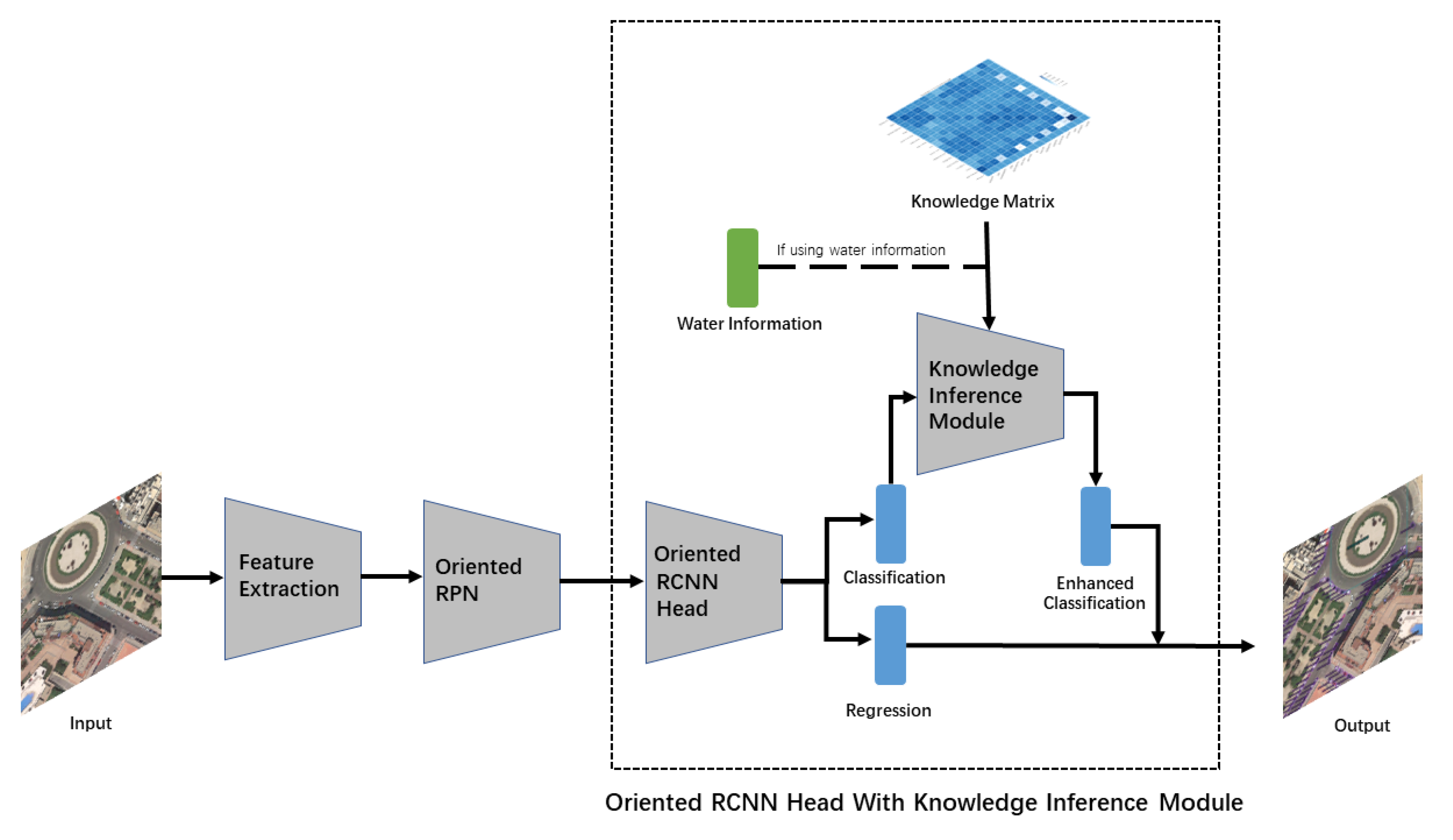
In this paper, we propose a knowledge-inferencing module that uses a residual structure to optimize the predicted class scores, which helps the detector to perform better. Our method can be applied to any two-stage object detection framework. In this work, we chose the Oriented R-CNN [15] as the framework and baseline model. The overall structure of the framework filled with the knowledge-aware bounding box head is presented in Figure 3.

4.1. Feature Extraction

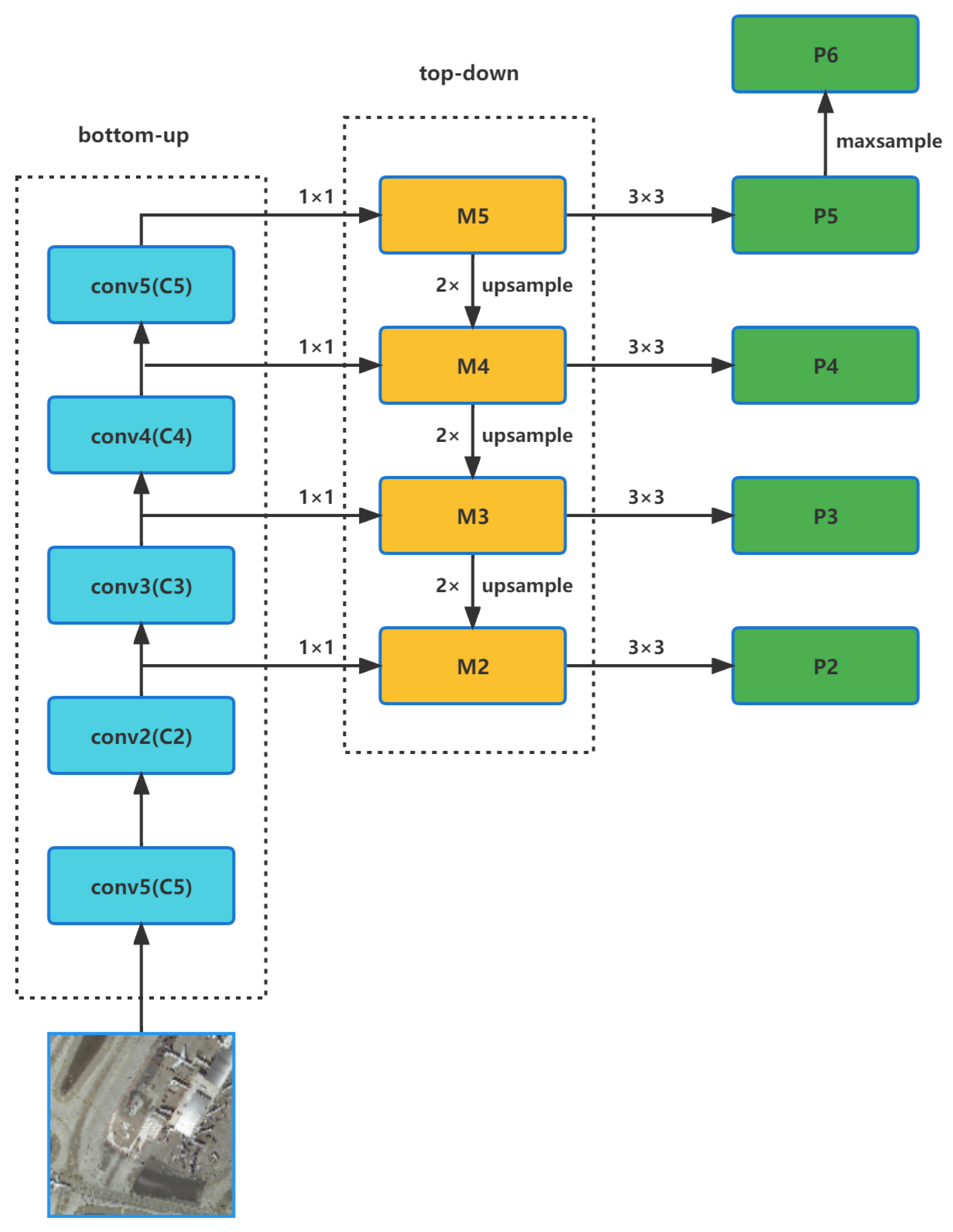
Resnet-50 [19] and FPN [34] are adopted into the Feature Extraction module to extract multi-scale features with which size-various objects can more easily be detected. Figure 4 shows the overall structure of the Feature Extraction module. In the bottom–up part, the input image is first input into a series of convolutional layers to generate low-semantic feature maps and high-semantic feature maps { C 1 , C 2 , C 3 , C 4 , C 5 }. Moreover, the top–down part obtains more powerful features by fusing features. To be specific, M 4 is equal to the sum of the result of the upsampling of M 5 and the result of the 1 × 1 convolution of C 4 . In this way, M 3 and M 2 are generated. P 2 , P 3 , P 4 , and P 5 are obtained by feeding M 2 , M 3 , M 4 , and M 5 into a 3 × 3 convolutional layer, and P 6 is obtained by maxpooling P 5 . Finally, this module outputs the fused multi-scale features { P 2 , P 3 , P 4 , P 5 , and P 6 }.

4.2. Oriented RPN

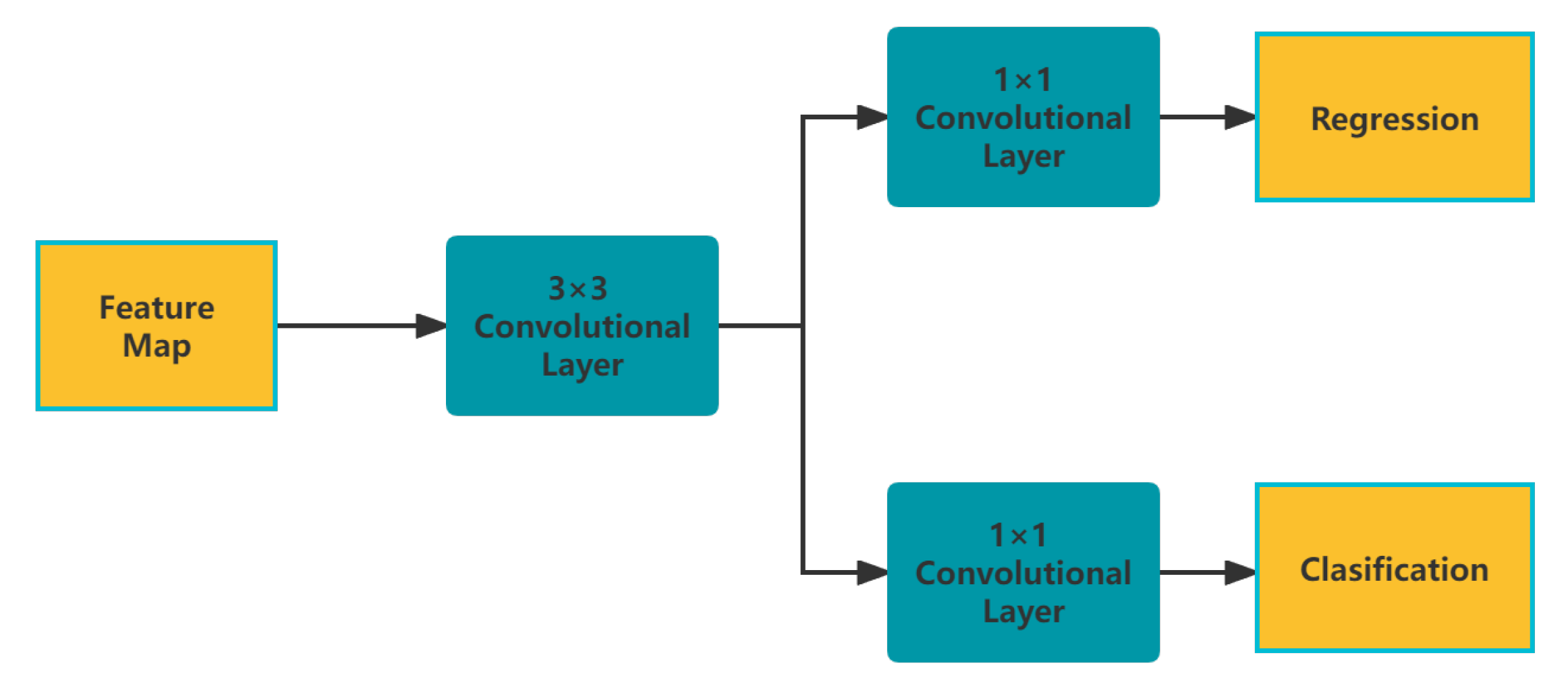
The oriented RPN takes { P 2 , P 3 , P 4 , P 5 , and P 6 } as the input and output region proposals with location information and an objectness score. Figure 5 shows the structure of the Oriented RPN.
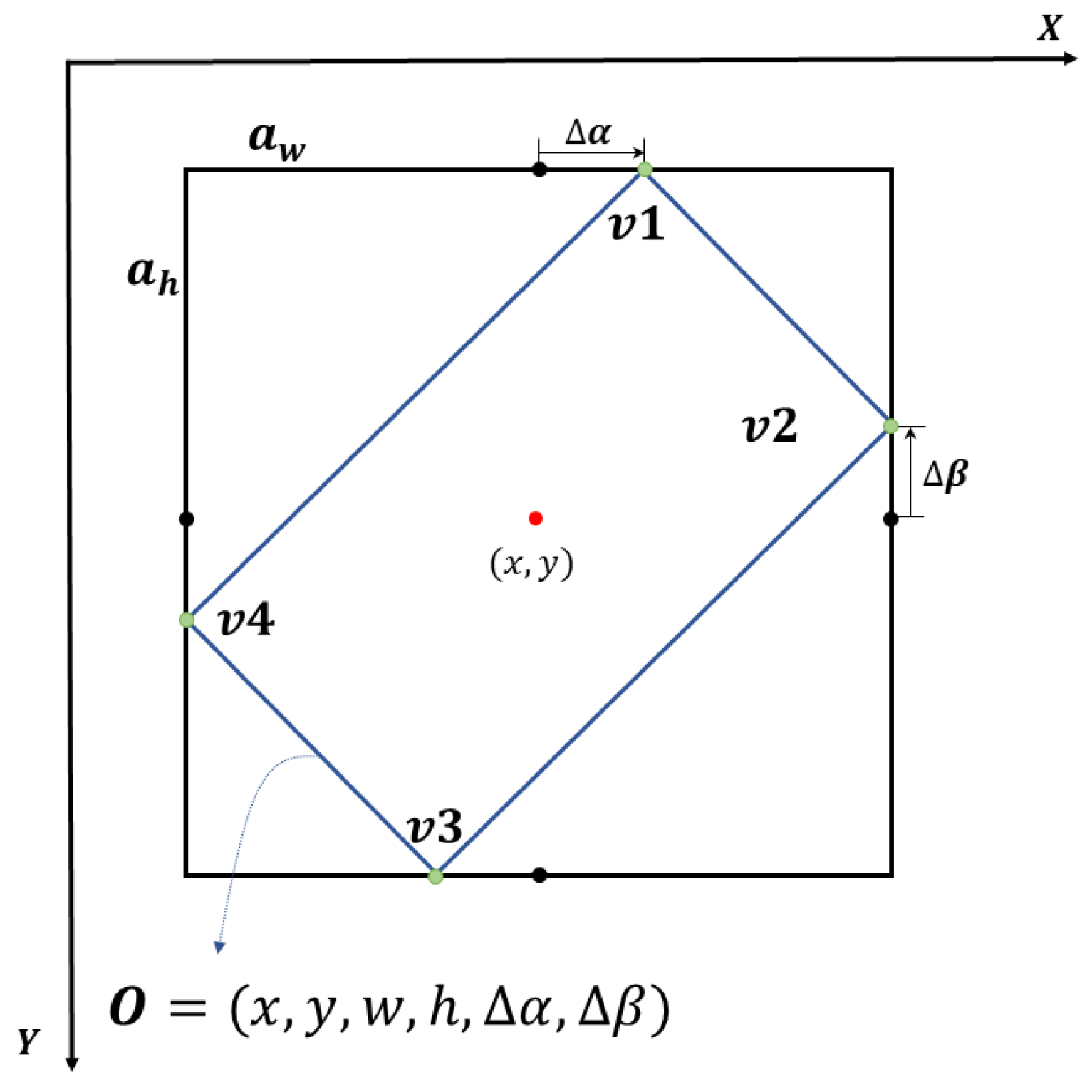
We set three horizontal anchors with aspect ratios of {1:2, 1:1, and 2:1} for every location in the features of all scales. The anchors correspond to { P 2 , P 3 , P 4 , P 5 , and P 6 } and have pixel areas of { 32 2 , 64 2 , 128 2 , 256 2 , and 512 2 }, which are represented by a 4-dimensional vector a = ( a x , a y , a w , a h ) . a x and a y denote the horizontal and vertical locations of the anchor center; a w and a h correspond to the width and height of the anchor. The upper branch of Figure 5, i.e., the regression branch, outputs the offset δ = ( δ x , δ y , δ w , δ h , δ α , δ β ) of proposals related to anchors. We decode the offset using Equation (8) to obtain oriented proposals ( x , y , w , h , Δ α , Δ β ) , where ( x , y ) denotes the location of the proposed center coordinate, w and h correspond to the width and height of the external rectangle box of the proposal, Δ α and Δ β denote the offsets of the proposal box vertex oriented to the midpoints of the top and right sides of the corresponding external rectangle. The lower branch of Figure 5, i.e., the classification branch, outputs objectness scores.
Δ α = δ α · w , Δ β = δ β · h w = a w · e δ w , h = a h · e δ h x = δ x · a w + a x , y = δ y · a h + a y
To represent the oriented object in elegant manner, the midpoint offset representation is introduced, the schematic of which is illustrated in Figure 6. In detail, the black horizontal box, i.e., the external rectangle of the blue one, is obtained from the anchor, where a w and a h are the width and height of the anchor, and the blue oriented box is the predicted oriented proposal box. The black dots and the light green dots are the midpoint of the external rectangle edges and the vertices of the oriented box, respectively. The predicted oriented proposal box can be represented as O = ( x , y , w , h , Δ α , Δ β ) , which can be computed by Equation (8). Furthermore, the vertices of predicted oriented proposal are denoted by a set of coordinates v 1 , v 2 , v 3 , v 4 . Similarly, Δ β is the distance between v 2 and the midpoint ( x , y h 2 ) of the top side, and because of the symmetry, the distance between v 3 and the midpoint ( x , y + h 2 ) of the bottom side equals Δ α . It is noticing that Δ α is distance between v 1 and the midpoint ( x , y h 2 ) of top side, and because of the symmetry distance between v 3 and the midpoint ( x , y + h 2 ) of bottom side equals to Δ α . Similarly, Δ β is the distance between v 2 and the midpoint ( x + w 2 , y ) of the right side, and the distance between v 4 and the midpoint ( x , y + h 2 ) of the left side equals Δ β . As a result, the vertices of the oriented proposal { v 1 , v 2 , v 3 , v 4 } can be computed using Equation (9).
v 1 = ( x , y h 2 ) + ( Δ α , 0 ) v 2 = ( x + w 2 , y ) + ( 0 , Δ β ) v 3 = ( x , y + h 2 ) + ( Δ α , 0 ) v 4 = ( x w 2 , y ) + ( 0 , Δ α )
In the training process, we assign positive and negative samples using the following rules:
  • An anchor that has an Intersection-over-Union(IoU) over 0.7 with any ground-truth box is regarded as a positive sample;
  • An anchor that has an IoU over 0.3 with a ground-truth box and the IoU is the highest;
  • An anchor that has an IoU lower than 0.3 is regarded as a negative sample;
  • Anchors that do not belong to the above cases are discarded during the training process.

4.3. Oriented RCNN Head with the Knowledge Inference Module

In this section, we apply our proposed Knowledge Inference module to the Oriented RCNN head in order to reduce missed and wrong detections by improving the predicted class scores. Specifically, the proposed module is applied on two kinds of knowledge: conditional co-occurrence knowledge and water area knowledge. Thus, the proposed module has two similar inferencing modes. The details can be seen in the middle part of Figure 3.
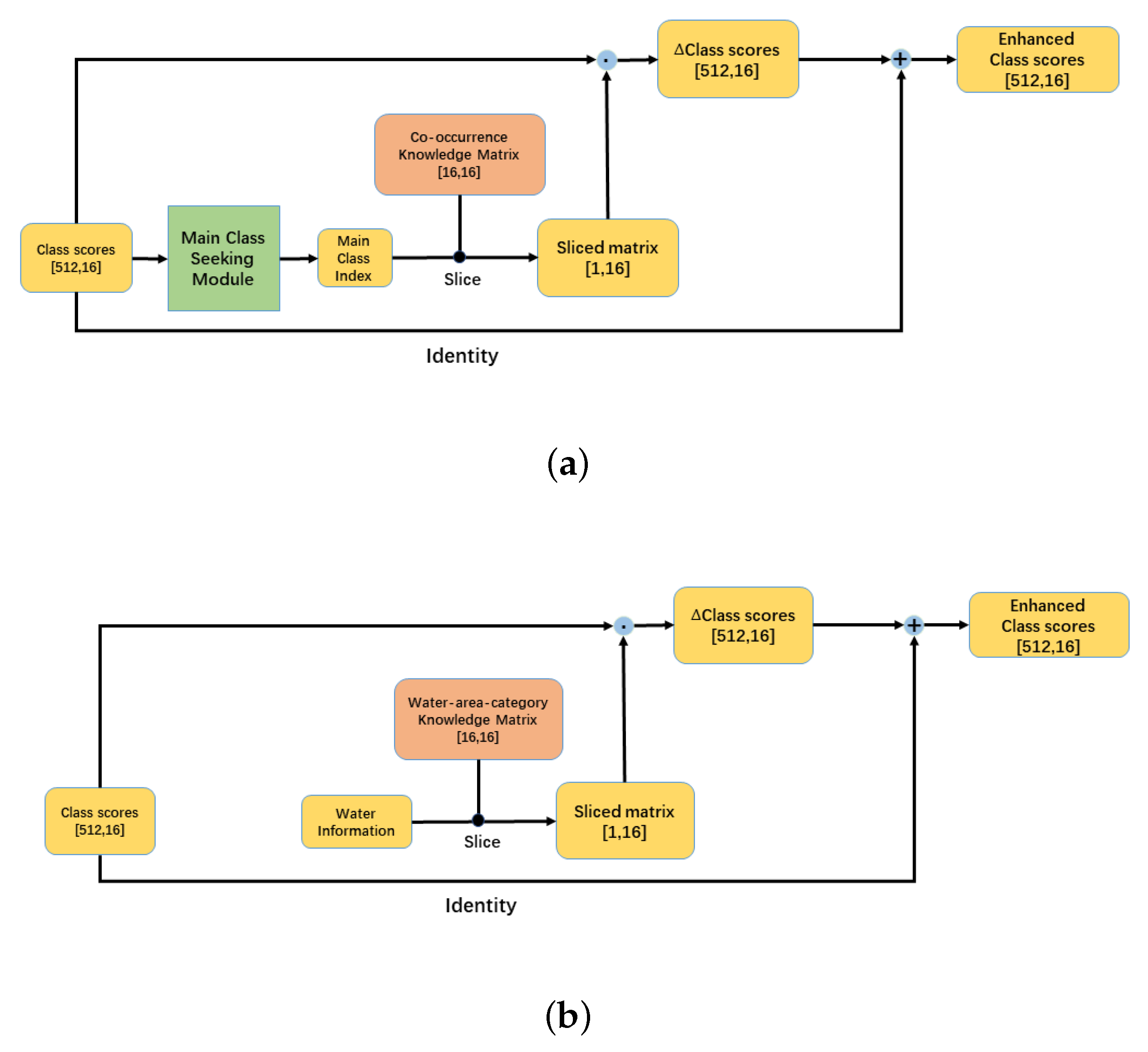
The oriented RCNN head first takes { P 2 , P 3 , P 4 , P 5 , and P 6 } and the oriented proposals from the oriented RPN as the input. In detail, feature vectors are obtained by rotating the RoI alignment to extract rotated RoI features according to the oriented proposals and transform them into fixed-length vectors. This is followed by two fully-connected layers. Then, we use two fully-connected sibling layers outputting classification scores and location predictions. For each image, we generate 512 predictions. Thus, the classification scores are denoted by the tensor of shape [ 512 , K + 1 ] , where K + 1 denotes the number of classes plus the background, and the location predictions are denoted by the tensor of shape [ 512 , 5 ] . With the aim of optimizing the predicted classification scores with the knowledge matrix, we propose the Knowledge Inference Module, the structure of which is illustrated in Figure 7. To be specific, Figure 7a shows the structure of the Knowledge Inference module applied to class conditional co-occurrence knowledge. The class scores [ 512 , 16 ] are first fed into the main-class-seeking-module to compute the major class in the image outputting the index of the main class. Then, the conditional co-occurrence matrix is sliced in terms of the main class index. The sliced matrix denotes the relationship between the main class and other classes, which is represented by the tensor of shape [ 1 , 16 ] . Therefore, the Δ class score is a tensor with knowledge integrated. It is obtained by dot-multiplying class scores [ 512 , 16 ] and transposing the sliced matrix [ 16 , 1 ] . However, our initial idea is to use knowledge to guide detection, so we apply a residual structure [19] into our proposed module, avoiding degradation brought about by using Δ class scores only. Enhanced class scores are the result of Δ class scores plus class scores. Additionally, the Knowledge Inference module on water area knowledge is shown in Figure 7b and is similar to that of the category conditional co-occurrence matrix. The difference is that the Main Class Seeking module and the main class index are replaced by water information showing whether there is a water area in the image.
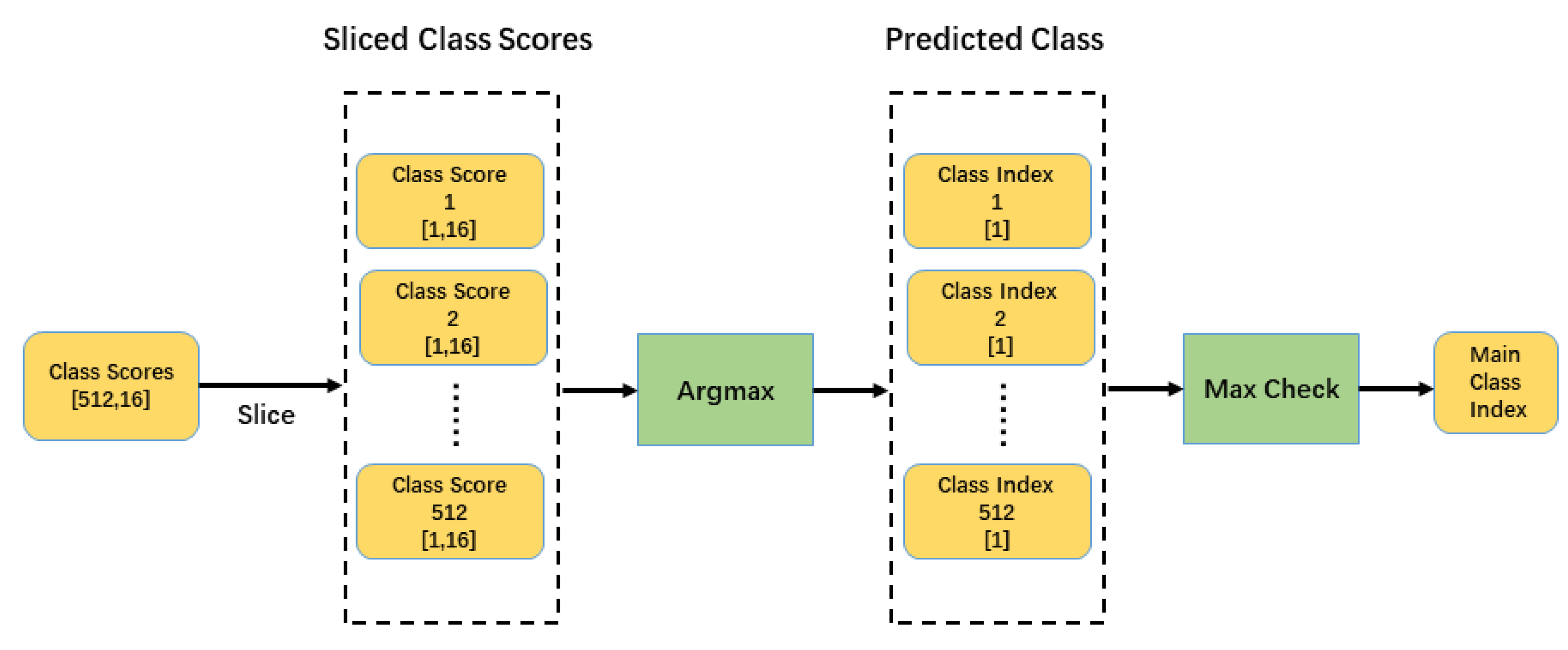
The structure of the Main-Class-Seeking module is illustrated in Figure 8. We first slice the tensor class scores [ 512 , 16 ] into 512 small tensors [ 1 , 16 ] and encode them into values of 1 to 512. Then, the sliced class scores are fed into the argmax() function outputting the classes with the highest classification scores. The function max check() is used to count the number of each category in the 512 predictions. This is performed sequentially, where the class with largest number is the main class.

4.4. Loss Function

To train the Oriented RPN and Oriented RCNN head, we introduce Cross-Entropy Loss L c l s for the classification task and Smooth L1 Loss L r e g for the regression task. The whole loss function L is defined as follows:
L ( p i , t i ) = 1 N i N L c l s ( p i , p i * ) + 1 N i N p i * L r e g ( t i , t i * )
L c l s ( p i , p i * ) = [ p i * l o g ( p i ) + ( 1 p i * ) l o g ( 1 p i ) ]
L r e g ( t i , t i * ) = 0.5 ( t i t i * ) 2 i f | t i t i * | < 1 | t i t i * | 0.5 o t h e r w i s e
where N and i are, respectively, the number and index of the predicted anchors in a image, p i is the probability of predicted anchors, p i * denotes the ground-truth label that belongs to { 0 , 1 } , i.e., negative and positive, and t i and t i * are the predicted box and the ground-truth box.

5. Experiments

In this section, we introduce the two geospatial object data sets used in this work. Then, evaluation metrics and implementation details are illustrated.

5.1. Data Sets

To evaluate the proposed method, we conduct experiments on two public aerial image data sets, i.e., DOTA and DIOR.
DOTA is the most popular large-scale data set for geospatial object detection, containing 2806 images and 188,282 instances with arbitrary-oriented objects. Moreover, there are 15 classes in the data set: bridge, harbor, ship, plane, helicopter, small vehicle, large vehicle, baseball diamond, ground track field, tennis court, basketball court, soccer ball field, roundabout, swimming pool, and storage tank. The image width ranges from 800 to 4000 pixels. In this work, the training set was used for training, and the validation set was used for evaluation.
DIOR is another data set that is widely used for geospatial object detection. It contains 23,463 optimal remote sensing images and 192,472 object instances annotated by a horizontal bounding box. There are 20 object classes in total, namely, airplane, airport, baseball field, basketball court, bridge, chimney, dam, expressway service area, expressway toll station, harbor, golf course, ground track field, overpass, ship, stadium, storage tank, tennis court, train station, vehicle, and windmill. The image size of the DIOR data set is 800 × 800 pixels. We trained the network on the training set and evaluated the method on the validation set.

5.2. Evaluation Metrics

To evaluate the performance of the proposed method, we utilized four popular evaluation metrics, i.e., precision, recall, average precision, and mean average precision, the calculation formulas of which are shown as follows:
P r e c i s i o n = T P T P + F P
R e c a l l = T P T P + F N
T N , F N , and F P denote the number of true positives, the number of false negatives, and the number of false positives, respectively. P r e c i s i o n measures the number of correctly identified positive detections of the total number of positive detections and R e c a l l measures the fraction of correctly identified positive detections of all positive samples.
A P is computed by calculating the average value of precision from recall = 0 to recall = 1.
A P = 0 1 P ( R ) d R
m A P is used to describe the multi-class object detection performance.
m A P = 1 N c l a s s j = 1 N c l a s s 0 1 P j ( R j ) d R j
where N c l a s s is the number of data set classes, j denotes the index of the class, and P j and R j are the precision rate and recall rate of the j-th class.

5.3. Implementation Details

The experiments were conducted on a single CPU, Intel Xeon CPU E5-2650 V4 at 2.20 GHz with a single GPU, NVIDIA Tesla P40 24 GB. The operating system was Ubuntu 18.04. The MMrotate [35] repository provided the training strategy. The size of the training image was 1024 × 1024, and the original DOTA images were split. All images in DIOR were 800 × 800 in size. Thus, there was no need to split the DIOR images. The objects in DIOR were annotated in the horizontal direction by the left-top vertex ( x 1 , y 1 ) and right-bottom vertex ( x 1 , y 1 ) . Thus, we converted the annotations into a form suitable for the Oriented RCNN: ( x 1 , y 1 , x 2 , y 1 , x 2 , y 2 , x 1 , y 2 ) , corresponding to the vertices of oriented ground truth box in clockwise order. As for the hyperparameters, the optimizer was the stochastic gradient descent (SGD) with a learning rate of 0.005, a momentum of 0.9, and a weight decay of 0.0001. The batch size was 1, and the number of training epochs was 12.

6. Results

In this section, the results of the experiments on DOTA and DIOR are displayed.

6.1. DOTA Results

We applied the knowledge inference module to two kinds of knowledge: class co-occurrence knowledge and water area knowledge. The results show that our method achieved increases in mAP of 1.0% and 0.6%, respectively. Table 3 reports the comparison between the baseline model Oriented RCNN and our proposed method, in which the proposed method basically maintains the performance for both kinds of knowledge and improves the accuracy of several classes, for example 8.7% for the term helicopter with conditional co-occurrence knowledge, and 2.9% for the soccer ball field with water area knowledge.
Table 3. Comparison between the baseline model Oriented RCNN and our proposed method on DOTA data set.
METHODPLBDBRGTFSVLVSHTCBCSTSBFRAHASPHCmAP
R 3 Det [17]88.867.444.169.062.971.778.789.947.361.247.459.359.251.724.361.5
CSL [7]88.172.239.863.864.371.978.589.652.461.050.566.056.650.127.562.2
S 2 A-net [9]89.172.045.664.865.074.879.590.160.267.349.362.260.653.437.664.8
FR-O [5]89.376.049.374.768.175.587.190.764.262.357.065.866.659.638.268.3
RoI Trans [6]89.976.548.173.168.778.288.790.873.662.762.063.473.757.247.970.3
Baseline [15]89.875.750.277.369.484.889.390.869.262.663.165.075.357.545.371.0
Water area89.675.650.376.468.484.389.490.772.962.666.067.275.656.548.871.6
Co-occurrence89.676.050.777.068.384.489.390.773.662.463.866.875.157.654.072.0
The baseline is the Oriented RCNN [15], the Water area denotes the Knowledge Inference module on water area knowledge, and Co-occurrence is the Knowledge Inference module applied on conditional co-occurrence knowledge, where: PL: plane, BD: baseball diamond, BR: bridge, GFT: ground field track, SV: small vehicle, LV: large vehicle, SH: ship, TC: tennis court, BC: basketball court, ST: storage tank, SBF: soccer ball field, RA: roundabout, HA: harbor, SP: swimming pool, and HC: helicopter.
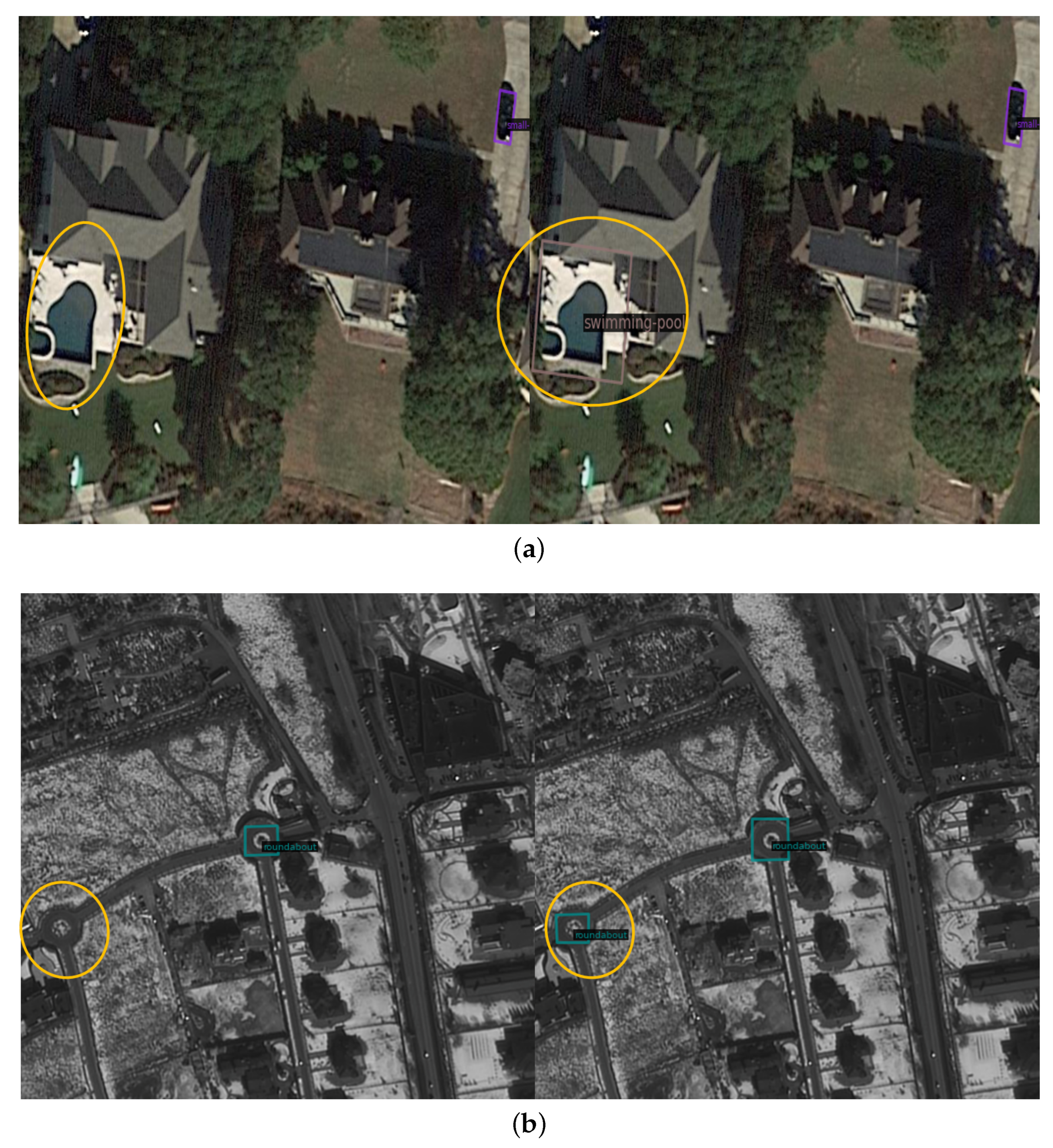
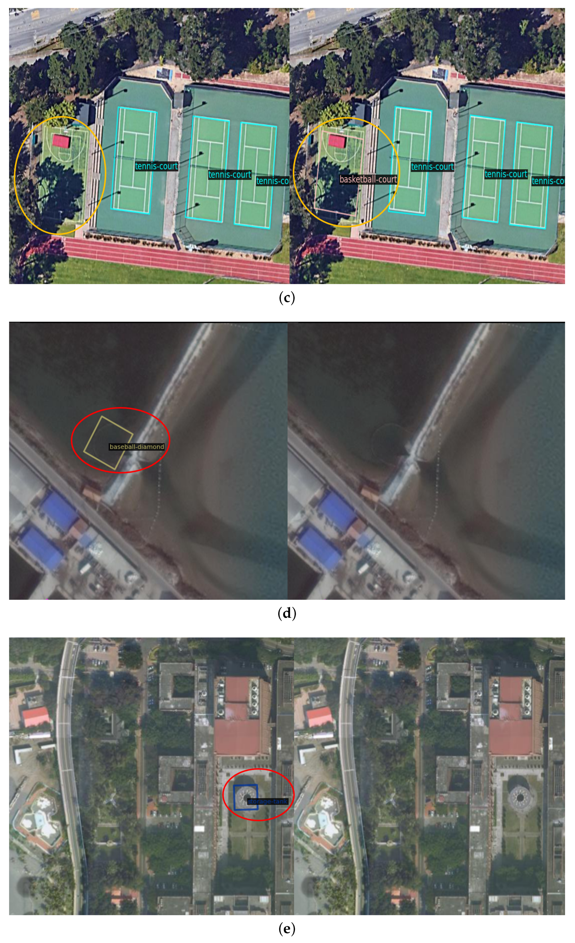
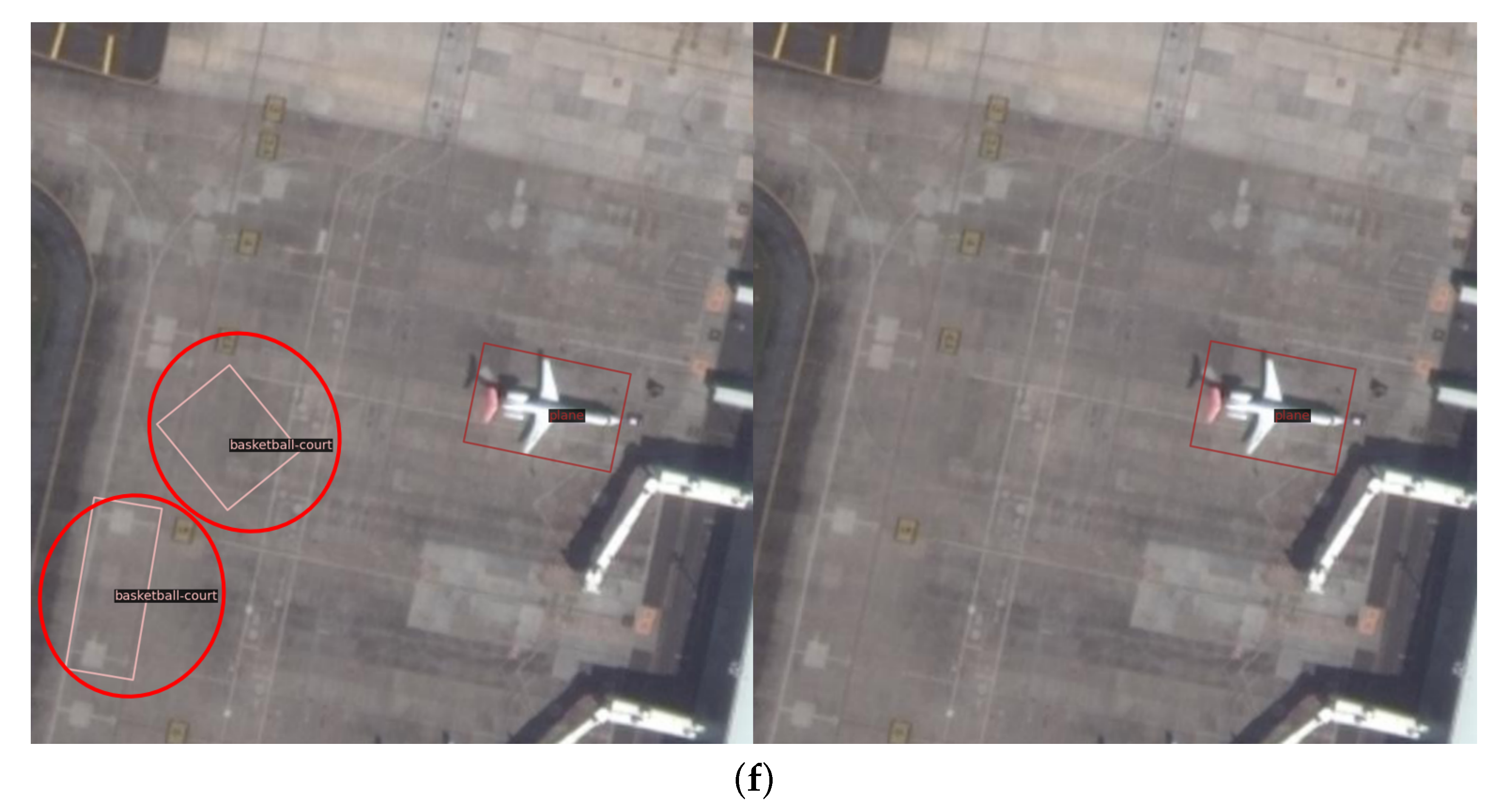
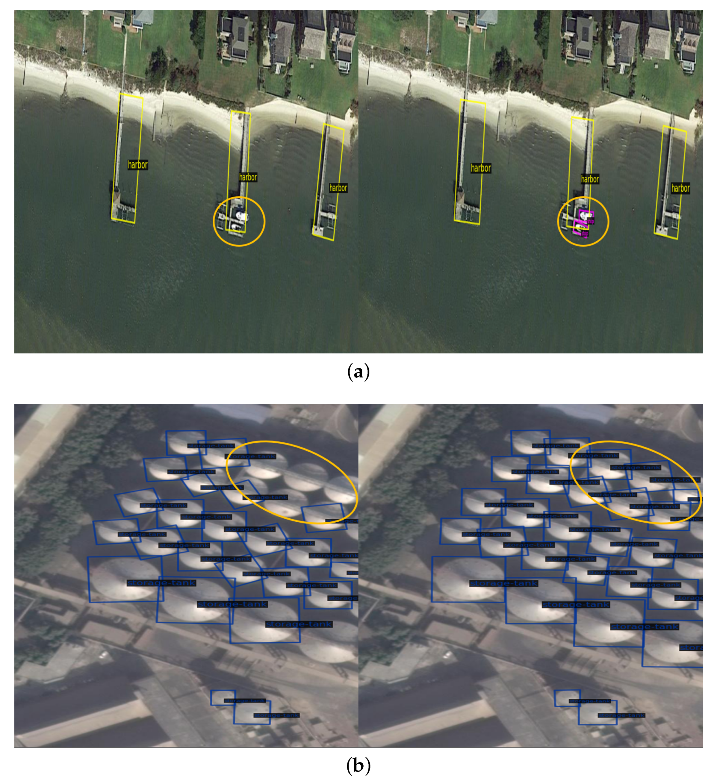
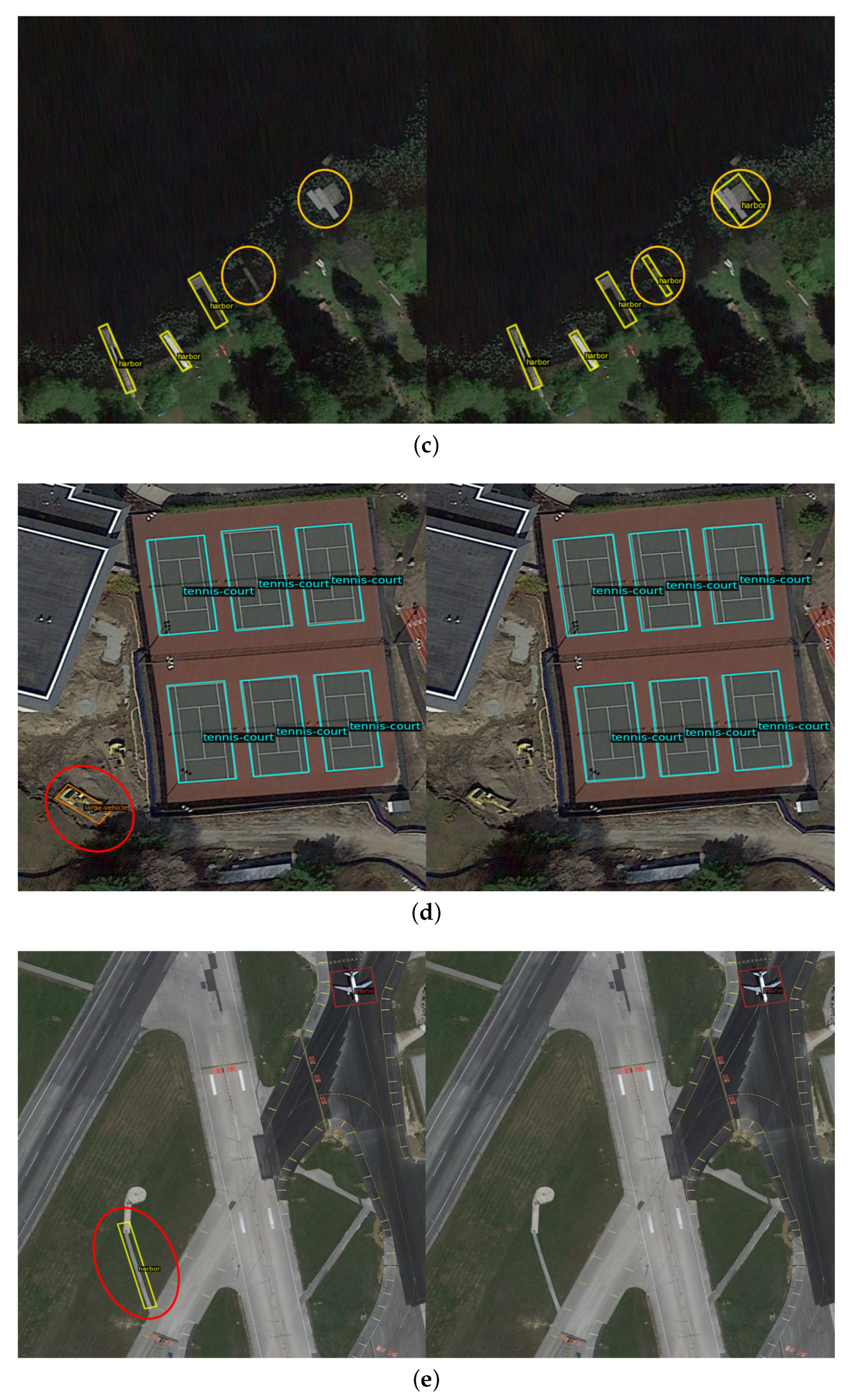
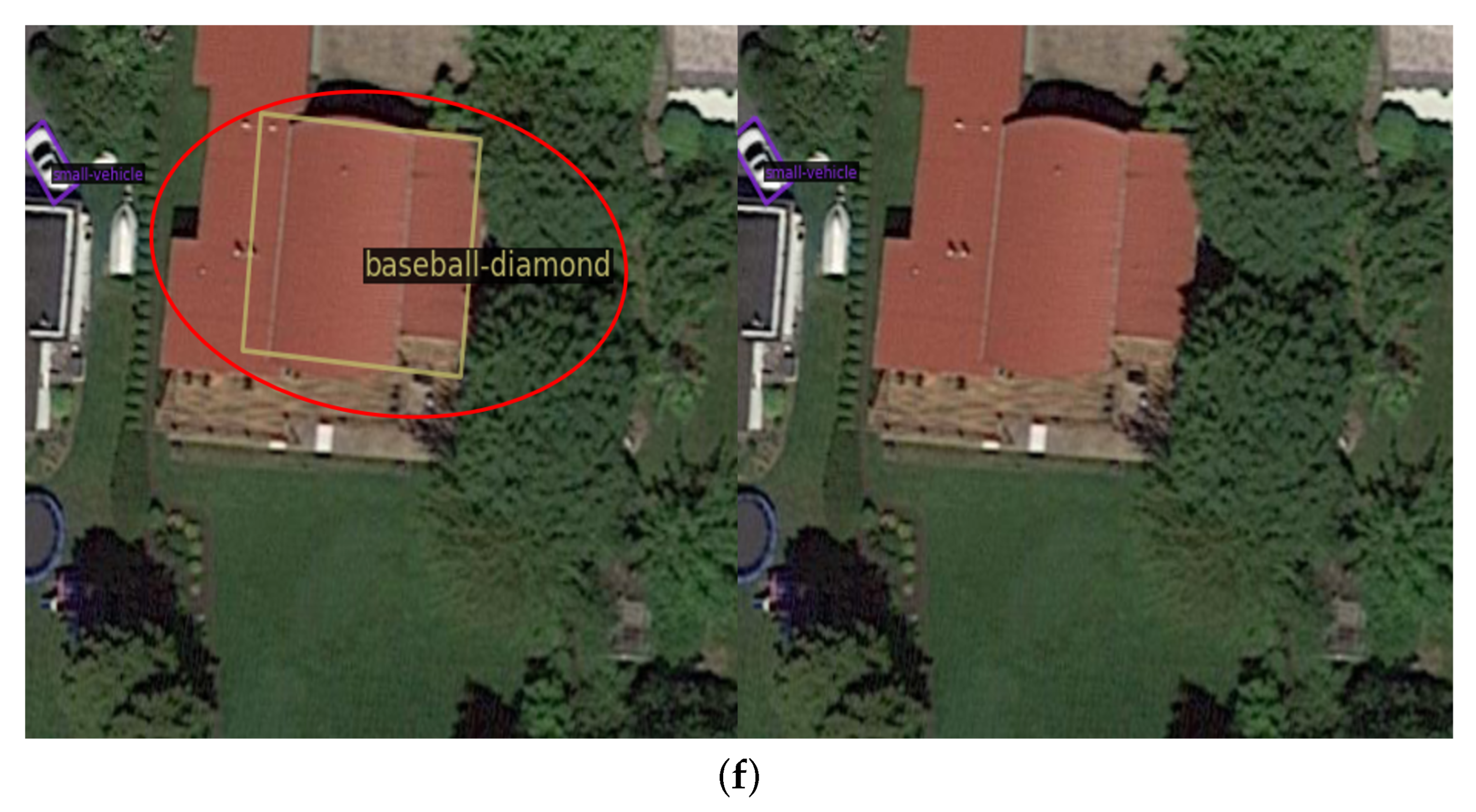
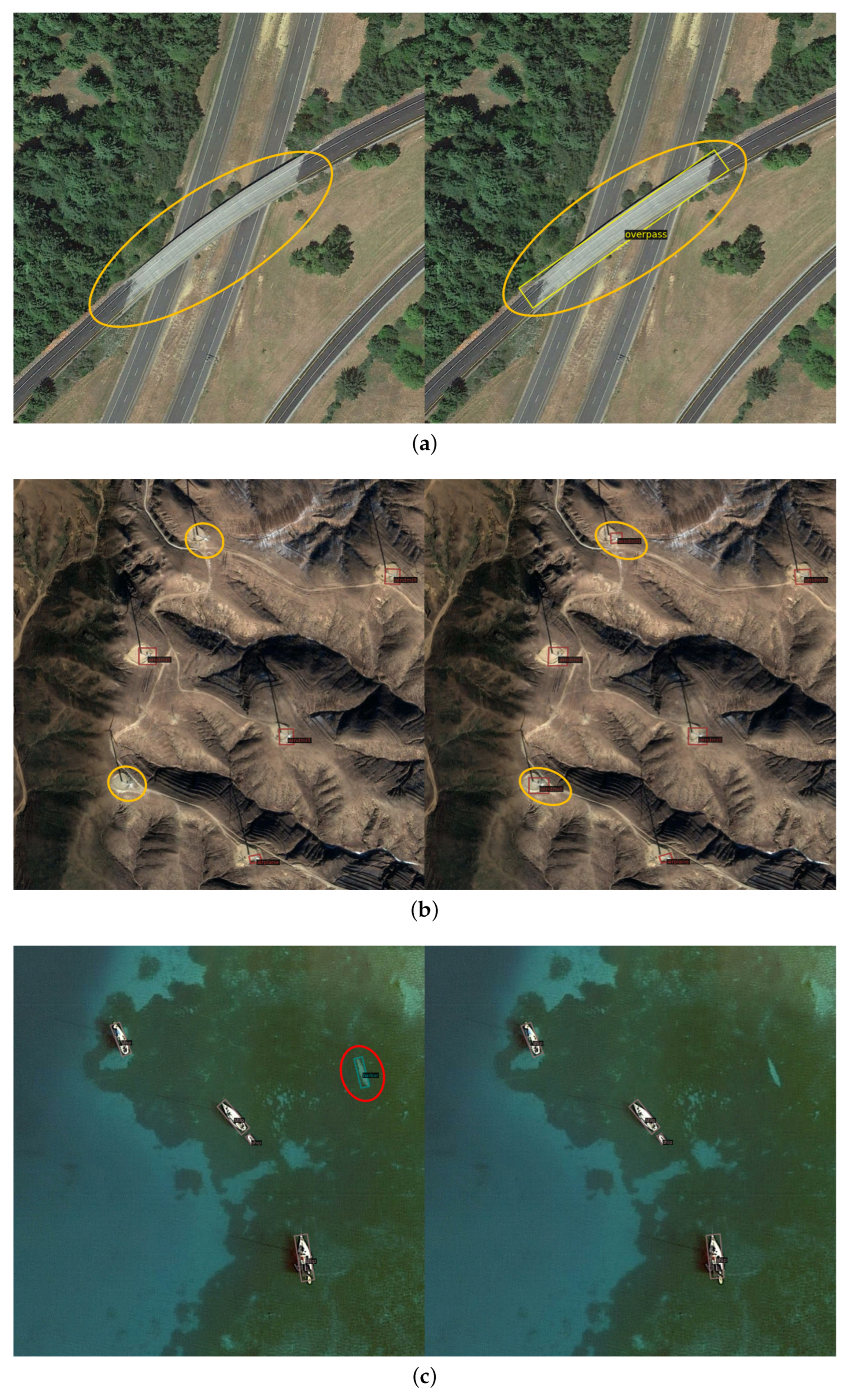
Moreover, to a certain degree, some missed detections and wrong detections were improved. Figure 9 and Figure 10 display the reductions in missed detection and wrong detection using conditional co-occurrence knowledge and water area knowledge, respectively. In each subfigure, the left half is the result of the baseline model and the right half is the result of the proposed method. We use yellow circles to draw missed detections and red circles to draw false detections. Additionally, the first three subfigures shown in Figure 9 and Figure 10 display missed detections, and the second three subfigures in Figure 9 and Figure 10 display the false detections. The positive detections are shown in Figure 11.
Improvement occurs due to the utilization of knowledge. On the one hand, knowledge is used to optimize the predicted class scores. Thus, the performance of the classification is promoted; on the other hand, the class predictions optimized by knowledge can help the network iterate better during backpropagation. As a result, the more powerful features can be extracted by the network.
In terms of the inferencing speed, we compared the baseline and Knowledge Inference module for two kinds of knowledge, as shown in Table 4. With the Knowledge Inference module, there was no significant drop in speed.

6.2. DIOR Results

The experiments conducted on the DIOR data set achieved a better performance. The ap values and mAP values are shown in Table 5. As can be seen, both kinds of knowledge had beneficial impacts on the detection performance, and the mAP values increased by 0.5% and 3.9%, respectively. Similarly, missed detections and wrong detections were effectively eliminated.
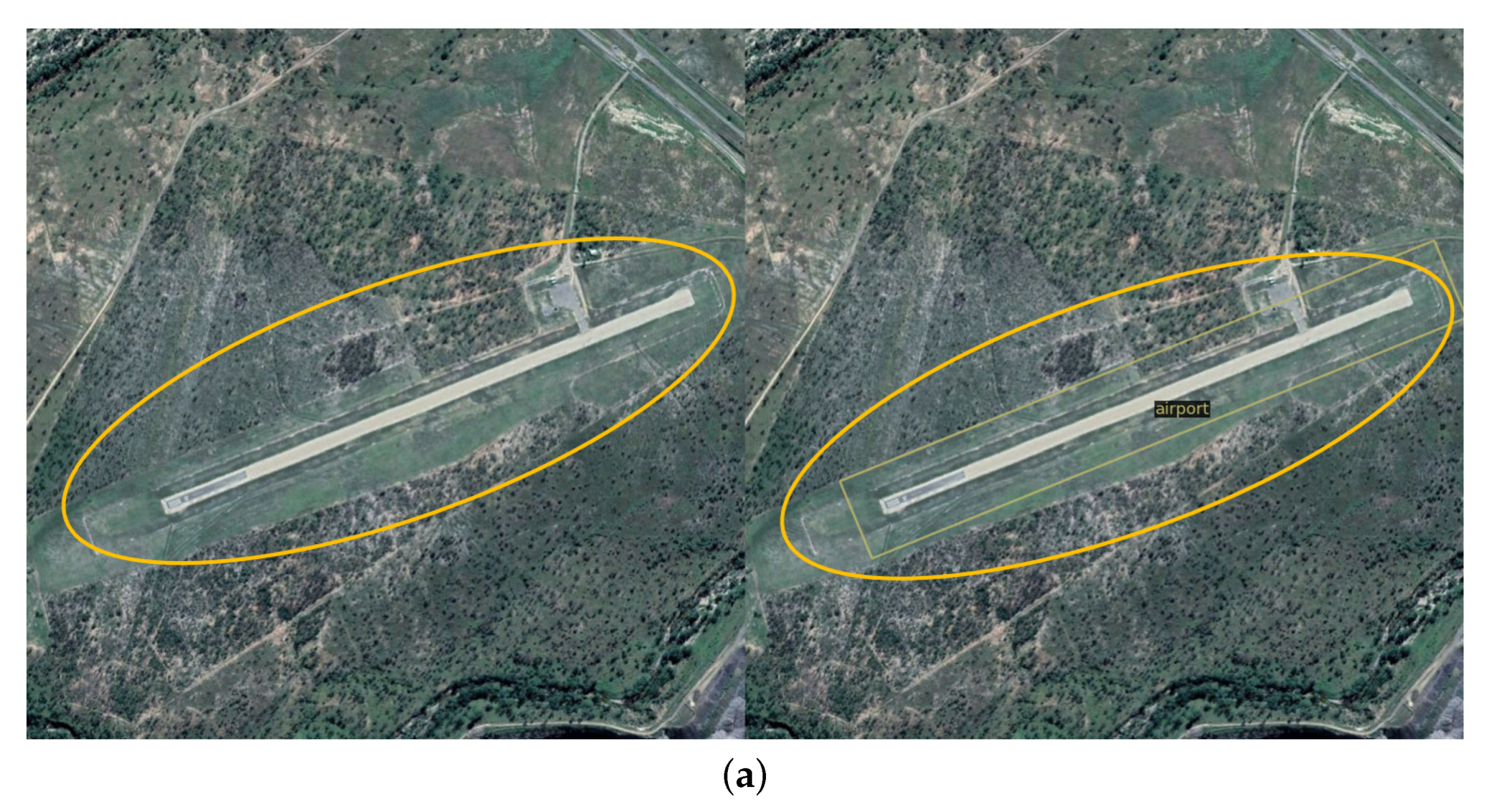
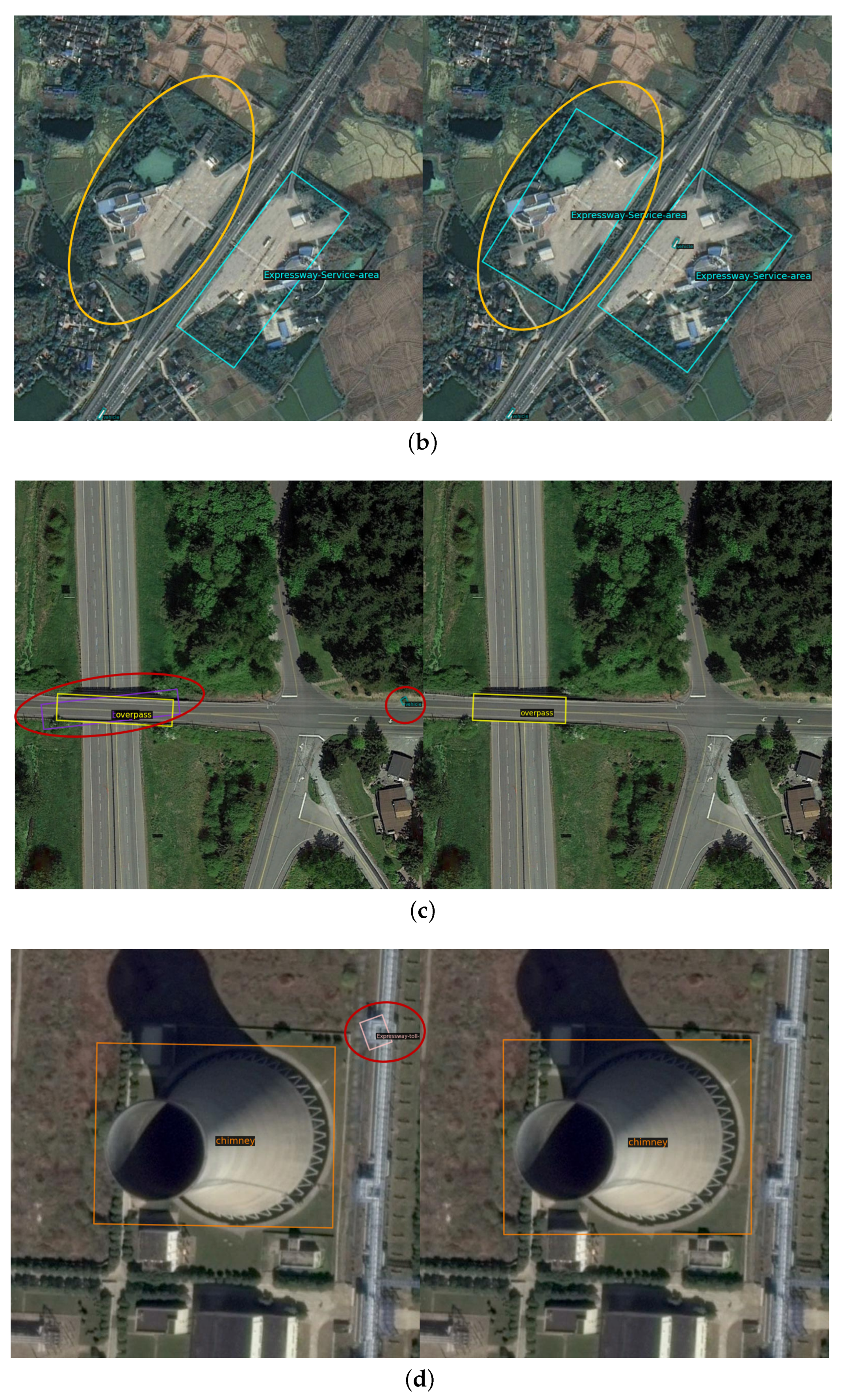
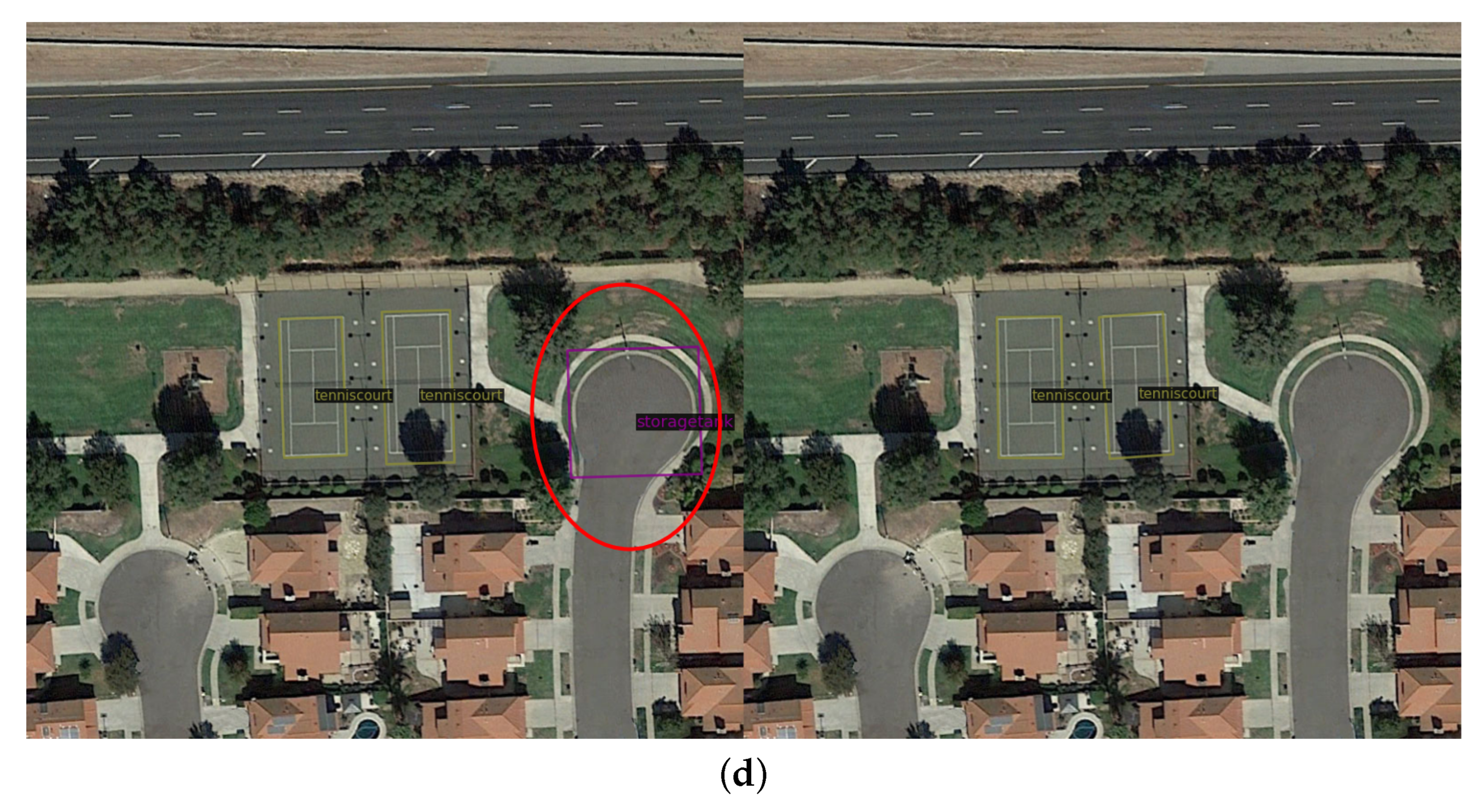
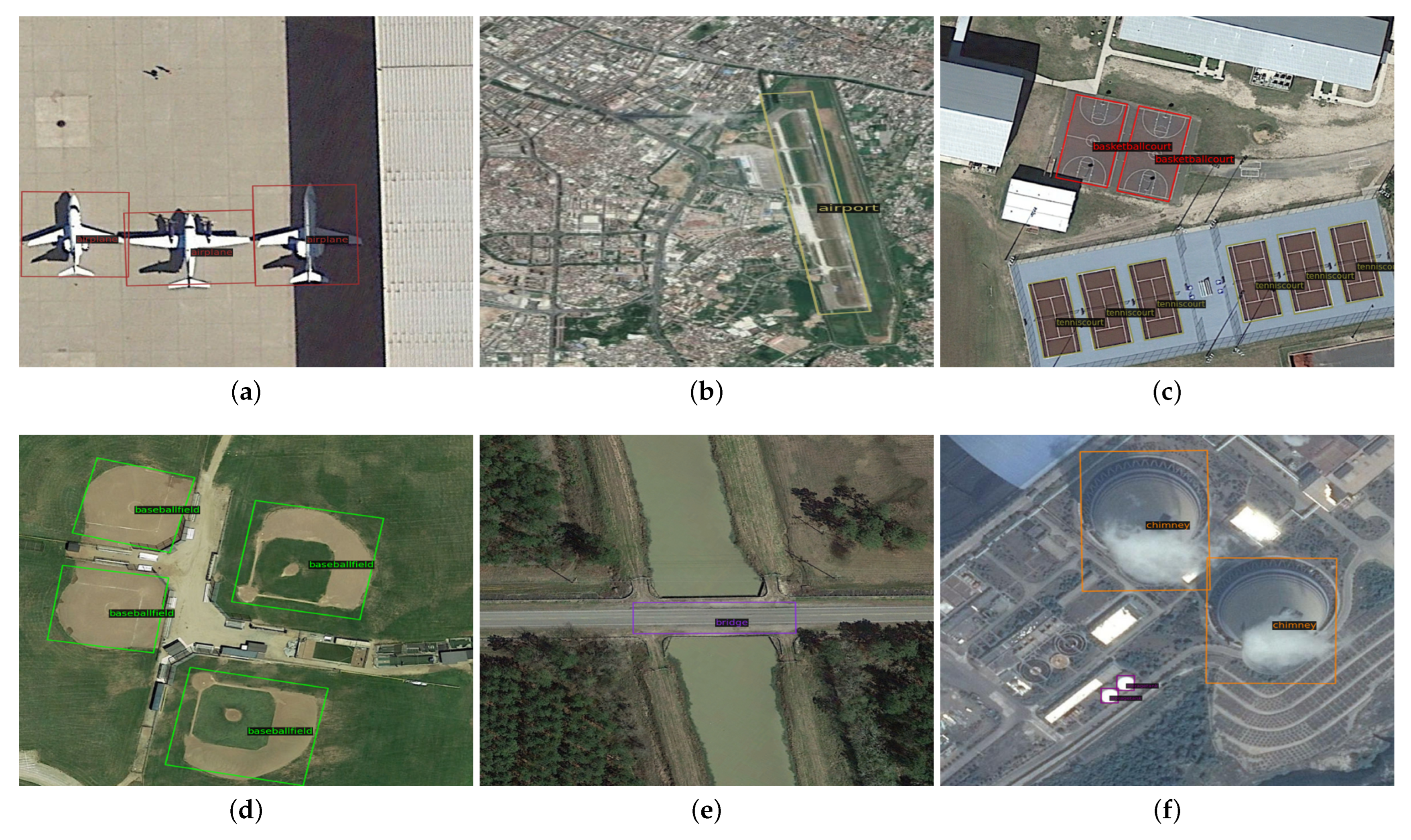
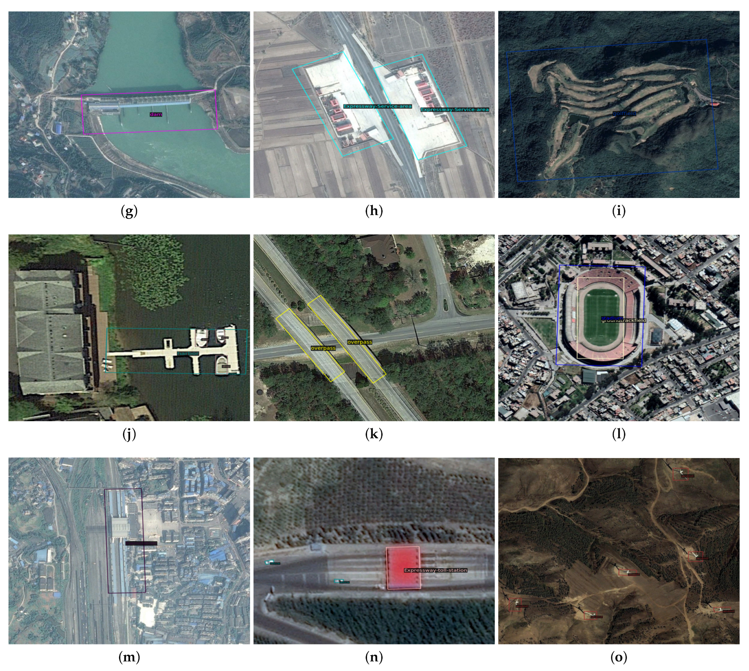
For the DIOR data set, we also visualized the impacts of two kinds of knowledge on the baseline, as shown in Figure 12 and Figure 13. As for the visualization of the DOTA data set, the yellow circle and red circle denote missed detections and false detections, respectively. The positive detections are shown in Figure 14.
A comparison of the inferencing speed and accuracy between the baseline and proposed methods for two kinds of knowledge is shown in Table 6. As can be seen, the Knowledge Inference module improved the detection accuracy with a negligible negative influence on the inferencing speed.

7. Conclusions

In this paper, in order to utilize knowledge to reduce false detections and missed detections caused by variation in the object appearance, varied object sizes, and complicated backgrounds, a series of steps were taken. We first established a knowledge matrix between the classes and a knowledge matrix between water areas and classes by analyzing the training set and proposed a novel equation, which can effectively avoid generalization degradation, to transform the relationship into form applicable for inferencing. Then, we proposed a method, the Knowledge Inference module, for integrating knowledge into object detection. The experiments were conducted on two public remote sensing data sets: DOTA and DIOR. The experimental results show that, compared to the baseline model, the proposed method achieved higher mAP values with fewer false detections and missed detections at an almost equal inferencing speed.

Author Contributions

Conceptualization, K.Z. and Y.D.; methodology, K.Z. and Y.D.; software, K.Z.; resources, W.X.; writing—original draft preparation, K.Z.; writing—review and editing, Y.D. and W.X.; visualization, K.Z. and Y.S.; supervision, P.H.; funding acquisition, Y.D. and W.X. All authors have read and agreed to the published version of the manuscript.

Funding

This research was funded by the Inner Mongolia Application Technology Research and Development Funding Project (2019GG138) and the Natural Science Foundation of the Inner Mongolia Autonomous Region (2020ZD18).

Data Availability Statement

Not applicable.

Conflicts of Interest

The authors declare no conflict of interest.

Appendix A

Table A1. The number of images where the category occurs N i m g ( l ) and the probabilities of class occurrences n ( l ) .
Object Categories N img ( l ) n ( l )
airplane3440.0586
airport3260.0556
baseball field5520.0941
basketball court3360.0573
bridge3780.0644
chimney2020.0344
dam2380.0406
expressway service area2790.0475
expressway toll station2850.0486
golf field2160.0368
ground track field5370.0916
harbor3290.0561
overpass4100.0699
ship6490.1107
stadium2890.0493
storage tank3900.0665
tennis court6050.1032
train station2440.0416
vehicle15610.2662
windmill4040.0689
Table A2. Probabilities of classes of DIOR appearing with water area and not appearing with water area. Column n ( l | w ) denotes the probability of category l appearing with water area; n ( l | w ¯ ) is the probability that category l appears with no water area.
Object Categories n ( l | w ) n ( l | w ¯ )
airplane0.04120.9588
airport0.44820.5518
baseball field0.07140.9286
basketball court0.09810.9019
bridge0.95250.0475
chimney0.12280.8772
dam10
expressway service area0.27190.7281
expressway toll station0.13350.8665
golf field0.91140.0886
ground track field0.12930.8707
harbor10
overpass0.11790.8821
ship0.99980.0002
stadium0.11260.8874
storage tank0.31260.6874
tennis court0.13660.8634
train station0.23980.7602
vehicle0.21400.7860
windmill0.04890.9511

References

  1. Cheng, G.; Han, J. A survey on object detection in optical remote sensing images. ISPRS J. Photogramm. Remote Sens. 2016, 117, 11–28. [Google Scholar] [CrossRef] [Green Version]
  2. Li, K.; Wan, G.; Cheng, G.; Meng, L.; Han, J. Object detection in optical remote sensing images: A survey and a new benchmark. ISPRS J. Photogramm. Remote Sens. 2020, 159, 296–307. [Google Scholar] [CrossRef]
  3. Wu, X.; Li, W.; Hong, D.; Tao, R.; Du, Q. Deep learning for unmanned aerial vehicle-based object detection and tracking: A survey. IEEE Geosci. Remote Sens. Mag. 2021, 10, 91–124. [Google Scholar] [CrossRef]
  4. Fascista, A. Toward Integrated Large-Scale Environmental Monitoring Using WSN/UAV/Crowdsensing: A Review of Applications, Signal Processing, and Future Perspectives. Sensors 2022, 22, 1824. [Google Scholar] [CrossRef] [PubMed]
  5. Mo, N.; Yan, L. Improved faster RCNN based on feature amplification and oversampling data augmentation for oriented vehicle detection in aerial images. Remote Sens. 2020, 12, 2558. [Google Scholar] [CrossRef]
  6. Ding, J.; Xue, N.; Long, Y.; Xia, G.S.; Lu, Q. Learning RoI transformer for oriented object detection in aerial images. In Proceedings of the IEEE/CVF Conference on Computer Vision and Pattern Recognition, Long Beach, CA, USA, 15–20 June 2019; pp. 2849–2858. [Google Scholar]
  7. Yang, X.; Yan, J. Arbitrary-oriented object detection with circular smooth label. In Proceedings of the European Conference on Computer Vision, Glasgow, UK, 23–28 August 2020; Springer: Berlin/Heidelberg, Germany, 2020; pp. 677–694. [Google Scholar]
  8. Guo, Z.; Liu, C.; Zhang, X.; Jiao, J.; Ji, X.; Ye, Q. Beyond bounding-box: Convex-hull feature adaptation for oriented and densely packed object detection. In Proceedings of the IEEE/CVF Conference on Computer Vision and Pattern Recognition, Nashville, TN, USA, 20–25 June 2021; pp. 8792–8801. [Google Scholar]
  9. Han, J.; Ding, J.; Li, J.; Xia, G.S. Align deep features for oriented object detection. IEEE Trans. Geosci. Remote Sens. 2021, 60, 1–11. [Google Scholar] [CrossRef]
  10. Torralba, A.; Oliva, A.; Castelhano, M.S.; Henderson, J.M. Contextual guidance of eye movements and attention in real-world scenes: The role of global features in object search. Psychol. Rev. 2006, 113, 766. [Google Scholar] [CrossRef] [PubMed] [Green Version]
  11. Li, Z.; Wu, Q.; Cheng, B.; Cao, L.; Yang, H. Remote sensing image scene classification based on object relationship reasoning CNN. IEEE Geosci. Remote Sens. Lett. 2020, 19, 1–5. [Google Scholar] [CrossRef]
  12. Xu, H.; Jiang, C.; Liang, X.; Lin, L.; Li, Z. Reasoning-rcnn: Unifying adaptive global reasoning into large-scale object detection. In Proceedings of the IEEE/CVF Conference on Computer Vision and Pattern Recognition, Long Beach, CA, USA, 15–20 June 2019; pp. 6419–6428. [Google Scholar]
  13. Xia, G.S.; Bai, X.; Ding, J.; Zhu, Z.; Belongie, S.; Luo, J.; Datcu, M.; Pelillo, M.; Zhang, L. DOTA: A large-scale dataset for object detection in aerial images. In Proceedings of the IEEE Conference on Computer Vision and Pattern Recognition, Salt Lake City, UT, USA, 18–23 June 2018; pp. 3974–3983. [Google Scholar]
  14. Fang, Y.; Kuan, K.; Lin, J.; Tan, C.; Chandrasekhar, V. Object detection meets knowledge graphs. In Proceedings of the International Joint Conferences on Artificial Intelligence, Melbourne, Australia, 19–25 August 2017. [Google Scholar]
  15. Xie, X.; Cheng, G.; Wang, J.; Yao, X.; Han, J. Oriented R-CNN for object detection. In Proceedings of the IEEE/CVF International Conference on Computer Vision, Montreal, QC, Canada, 10–17 October 2021; pp. 3520–3529. [Google Scholar]
  16. Ming, Q.; Miao, L.; Zhou, Z.; Dong, Y. CFC-Net: A critical feature capturing network for arbitrary-oriented object detection in remote-sensing images. IEEE Trans. Geosci. Remote Sens. 2021, 60, 1–14. [Google Scholar] [CrossRef]
  17. Yang, X.; Yan, J.; Feng, Z.; He, T. R3det: Refined single-stage detector with feature refinement for rotating object. In Proceedings of the AAAI Conference on Artificial Intelligence, Vancouver, BC, Canada, 2–9 February 2021; Volume 35, pp. 3163–3171. [Google Scholar]
  18. Han, J.; Ding, J.; Xue, N.; Xia, G.S. Redet: A rotation-equivariant detector for aerial object detection. In Proceedings of the IEEE/CVF Conference on Computer Vision and Pattern Recognition, Nashville, TN, USA, 19–15 June 2021; pp. 2786–2795. [Google Scholar]
  19. He, K.; Zhang, X.; Ren, S.; Sun, J. Deep residual learning for image recognition. In Proceedings of the IEEE Conference on Computer Vision and Pattern Recognition, Las Vegas, NV, USA, 27–30 June 2016; pp. 770–778. [Google Scholar]
  20. Chen, C.; Gong, W.; Chen, Y.; Li, W. Object detection in remote sensing images based on a scene-contextual feature pyramid network. Remote Sens. 2019, 11, 339. [Google Scholar] [CrossRef]
  21. Liu, Y.; Wang, R.; Shan, S.; Chen, X. Structure inference net: Object detection using scene-level context and instance-level relationships. In Proceedings of the IEEE Conference on Computer Vision and Pattern Recognition, Salt Lake City, UT, USA, 18–23 June 2018; pp. 6985–6994. [Google Scholar]
  22. Siris, A.; Jiao, J.; Tam, G.K.; Xie, X.; Lau, R.W. Scene context-aware salient object detection. In Proceedings of the IEEE/CVF International Conference on Computer Vision, Montreal, QC, Canada, 10–17 October 2021; pp. 4156–4166. [Google Scholar]
  23. Vaswani, A.; Shazeer, N.; Parmar, N.; Uszkoreit, J.; Jones, L.; Gomez, A.N.; Kaiser, Ł.; Polosukhin, I. Attention is all you need. Adv. Neural Inf. Processing Syst. 2017, 30. [Google Scholar] [CrossRef]
  24. Li, K.; Cheng, G.; Bu, S.; You, X. Rotation-insensitive and context-augmented object detection in remote sensing images. IEEE Trans. Geosci. Remote Sens. 2017, 56, 2337–2348. [Google Scholar] [CrossRef]
  25. Zhang, G.; Lu, S.; Zhang, W. CAD-Net: A context-aware detection network for objects in remote sensing imagery. IEEE Trans. Geosci. Remote Sens. 2019, 57, 10015–10024. [Google Scholar] [CrossRef] [Green Version]
  26. Zhang, K.; Wu, Y.; Wang, J.; Wang, Y.; Wang, Q. Semantic context-aware network for multiscale object detection in remote sensing images. IEEE Geosci. Remote Sens. Lett. 2021, 19, 1–5. [Google Scholar] [CrossRef]
  27. Liu, J.; Li, S.; Zhou, C.; Cao, X.; Gao, Y.; Wang, B. SRAF-Net: A Scene-Relevant Anchor-Free Object Detection Network in Remote Sensing Images. IEEE Trans. Geosci. Remote Sens. 2021, 60, 1–14. [Google Scholar] [CrossRef]
  28. Feng, X.; Han, J.; Yao, X.; Cheng, G. TCANet: Triple context-aware network for weakly supervised object detection in remote sensing images. IEEE Trans. Geosci. Remote Sens. 2020, 59, 6946–6955. [Google Scholar] [CrossRef]
  29. Cheng, B.; Li, Z.; Xu, B.; Dang, C.; Deng, J. Target detection in remote sensing image based on object-and-scene context constrained CNN. IEEE Geosci. Remote Sens. Lett. 2021, 19, 1–5. [Google Scholar] [CrossRef]
  30. Xu, H.; Jiang, C.; Liang, X.; Li, Z. Spatial-aware graph relation network for large-scale object detection. In Proceedings of the IEEE/CVF Conference on Computer Vision and Pattern Recognition, Long Beach, CA, USA, 15–20 June 2019; pp. 9298–9307. [Google Scholar]
  31. Xu, H.; Fang, L.; Liang, X.; Kang, W.; Li, Z. Universal-rcnn: Universal object detector via transferable graph r-cnn. In Proceedings of the AAAI Conference on Artificial Intelligence, New York, NY, USA, 7–12 February 2020; Volume 34, pp. 12492–12499. [Google Scholar]
  32. Shu, X.; Liu, R.; Xu, J. A Semantic Relation Graph Reasoning Network for Object Detection. In Proceedings of the 2021 IEEE 10th Data Driven Control and Learning Systems Conference (DDCLS), Suzhou, China, 14–16 May 2021; IEEE: Piscataway, NJ, USA, 2021; pp. 1309–1314. [Google Scholar]
  33. Jiang, C.; Xu, H.; Liang, X.; Lin, L. Hybrid knowledge routed modules for large-scale object detection. Adv. Neural Inf. Processing Syst. 2018, 31. [Google Scholar] [CrossRef]
  34. Lin, T.Y.; Dollár, P.; Girshick, R.; He, K.; Hariharan, B.; Belongie, S. Feature pyramid networks for object detection. In Proceedings of the IEEE Conference on Computer Vision and Pattern Recognition, Honolulu, HI, USA, 21–26 July 2017; pp. 2117–2125. [Google Scholar]
  35. Zhou, Y.; Yang, X.; Zhang, G.; Wang, J.; Liu, Y.; Hou, L.; Jiang, X.; Liu, X.; Yan, J.; Lyu, C.; et al. MMRotate: A Rotated Object Detection Benchmark using PyTorch. arXiv 2022, arXiv:2204.13317. [Google Scholar]
Figure 1. False detection in red circle and missed detection in yellow circle: (a) false detection of a helicopter and harbor; (b) false detection of a soccer ball field; (c) missed detection of a basketball court; (d) missed detection of a bridge.
Remotesensing 14 06103 g001
Figure 2. Relationships between the ship, harbor, and water assembled in the knowledge pool.
Remotesensing 14 06103 g002
Figure 3. The overall structure of the framework filled with the Knowledge Inference module, a two-stage detector. Feature extraction module first extracts multi-scale features fed into the Oriented RPN. Region proposals are generated by the Oriented RPN and used for classifying and regression in the Oriented RCNN head. Finally, the classification scores are fed into the Knowledge Inference Module, resulting in knowledge-enhanced classification scores.
Remotesensing 14 06103 g003
Figure 4. The overall structure of the Feature Extraction module.
Remotesensing 14 06103 g004
Figure 5. The structure of the Oriented RPN, which contains a 3 × 3 convolutional layer and two sibling 1 × 1 convolutional layers for classification and regression, respectively.
Remotesensing 14 06103 g005
Figure 6. Schematic of the midpoint offset scheme.
Remotesensing 14 06103 g006
Figure 7. Structures of the Knowledge Inference module applied on two kinds of knowledge: (a) the structure of the Knowledge Inference module applied on conditional co-occurrence knowledge; (b) the structure of the Knowledge Inference module applied on water area knowledge.
Remotesensing 14 06103 g007
Figure 8. The Main Class Seeking module consists of a slice operation, argmax() function and a max check() function.
Remotesensing 14 06103 g008
Figure 9. Visualization of the results of the Knowledge Inference module applied to category occurrence knowledge. (a) missed detection of swimming pools; (b) missed detection of roundabouts; (c) missed detection of basketball courts; (d) false detection of baseball diamonds; (e) false detection of storage tanks; (f) false detection of basketball courts.
Remotesensing 14 06103 g009aRemotesensing 14 06103 g009bRemotesensing 14 06103 g009c
Figure 10. Visualization of the results of the Knowledge Inference module applied to water area knowledge. (a) missed detections of ships in the middle of the image; (b) missed detection storage tanks; (c) missed detection of harbors; (d) false detection of large vehicles; (e) false detection of harbors; (f) false detection of baseball diamonds.
Remotesensing 14 06103 g010aRemotesensing 14 06103 g010bRemotesensing 14 06103 g010c
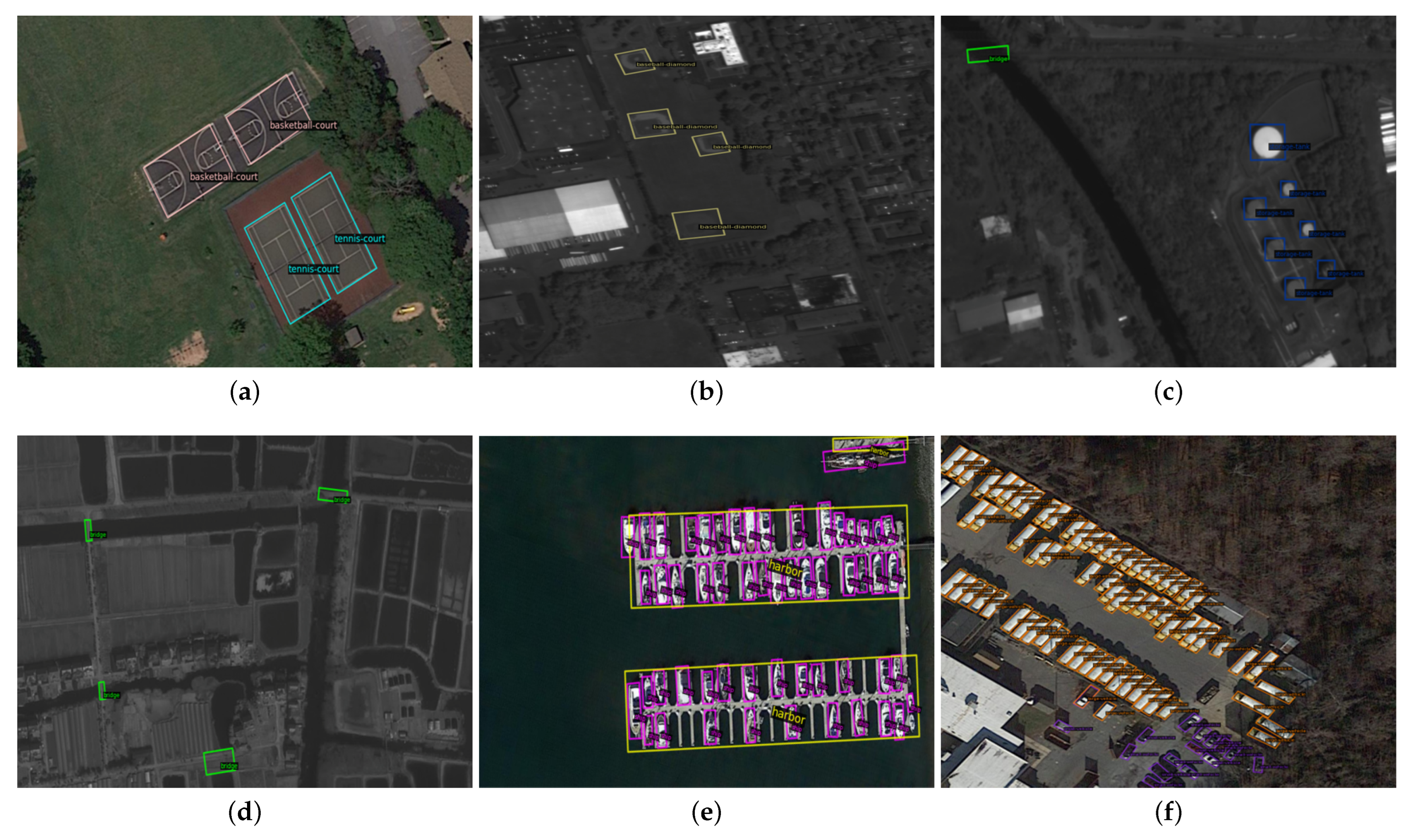
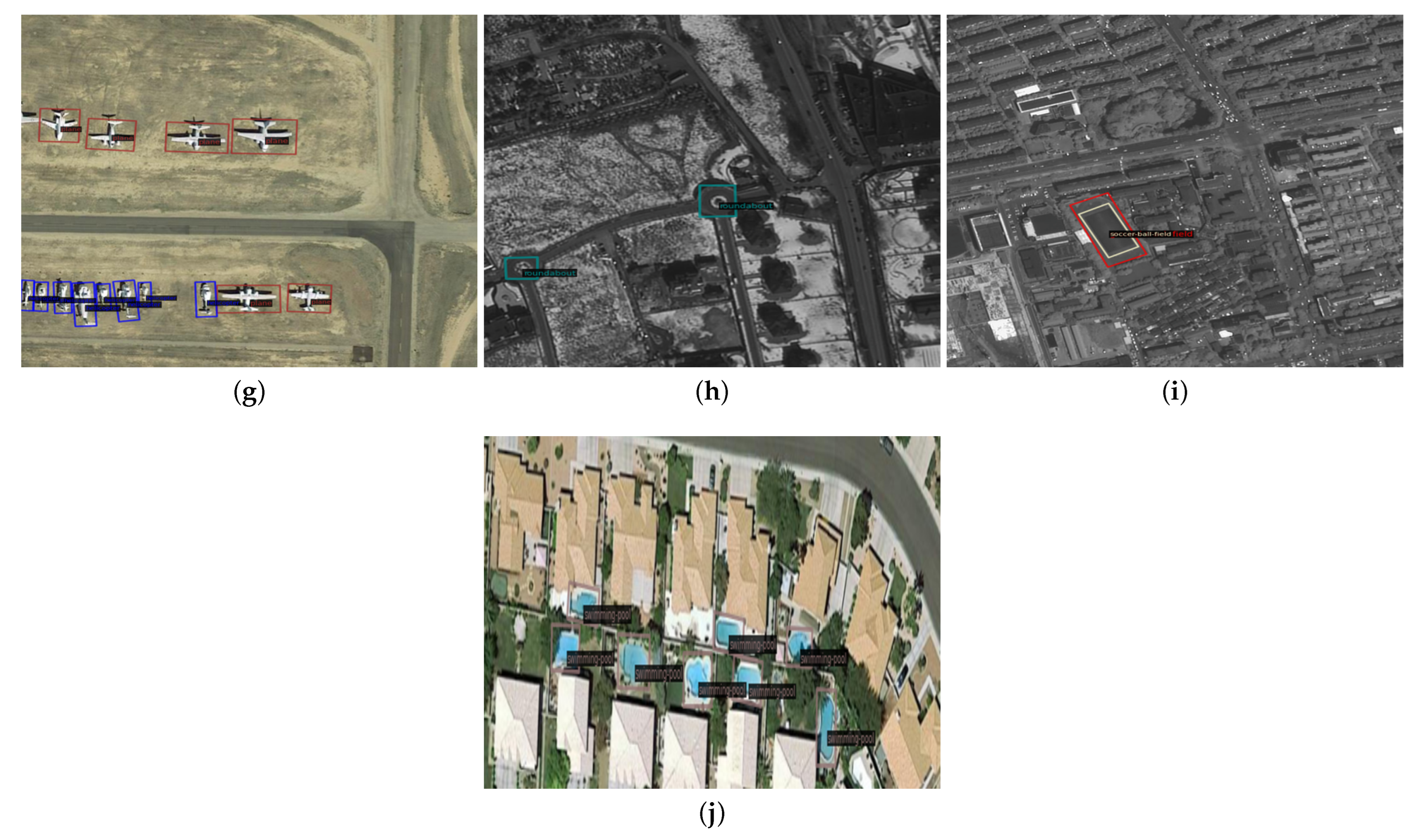
Figure 11. Visualization of the positive results. (a) basketball courts and tennis courts; (b) baseball diamonds; (c) bridge and storage tanks; (d) bridges; (e) harbors and ships; (f) large vehicles and small vehicles; (g) planes and helicopters; (h) roundabouts; (i) ground field tracks and soccer ball fields; (j) swimming pools.
Remotesensing 14 06103 g011aRemotesensing 14 06103 g011b
Figure 12. Visualization of the results of the Knowledge Inference module applied on category occurrence knowledge: (a) missed detection of airports; (b) missed detection of expressway service areas; (c) false detection of bridges in the purple box and vehicles; (d) false detection of expressway toll stations.
Remotesensing 14 06103 g012aRemotesensing 14 06103 g012b
Figure 13. Visualization of the results of the Knowledge Inference module applied on category occurrence knowledge. (a) missed detection of overpasses; (b) missed detection of windmills; (c) false detection of harbors; (d) false detection of storage tanks.
Remotesensing 14 06103 g013aRemotesensing 14 06103 g013b
Figure 14. Visualization of the positive results. (a) airplanes; (b) airports; (c) basketball courts and tennis courts; (d) baseball fields; (e) bridges; (f) chimneys and storage tanks; (g) dams; (h) expressway service areas; (i) golf fields; (j) harbors and ships; (k) overpasses; (l) ground track fields and stadiums; (m) train stations; (n) expressway toll stations; (o) windmills.
Remotesensing 14 06103 g014aRemotesensing 14 06103 g014b
Table 1. The number of images in which the category occurs N i m g ( l ) and the probabilities of the class occurrence n ( l ) .
Object Categories N img ( l ) n ( l )
Plane1970.1396
Baseball diamond1220.0864
Bridge2100.1488
Ground track field1770.1254
Small vehicle4860.3444
Large vehicle3800.2693
Ship3260.2310
Tennis court3020.2140
Basketball court1110.0786
Storage tank1610.1141
Soccer ball field1360.0963
Roundabout1700.1204
Harbor3390.2402
Swimming pool1440.1020
Helicopter300.0212
Table 2. Probabilities of classes appearing with water area and not with water area. Column n ( l | w ) denotes the probability of category l appearing with water area; n ( l | w ¯ ) is the probability of category l not appearing with water area.
Object Categories n ( l | w ) n ( l | w ¯ )
plane0.17480.8252
baseball-diamond0.55430.4457
bridge0.97550.0245
ground-track-field0.64620.3538
small-vehicle0.28370.7163
large-vehicle0.15840.8416
ship0.99940.0006
tennis-court0.29450.7055
basketball-court0.25440.7456
storage-tank0.94020.0598
soccer-ball-field0.52150.4785
roundabout0.61660.3834
harbor10
swimming-pool10
helicopter0.00150.9985
Table 4. Comparison of the inferencing speed and accuracy between the baseline and proposed methods for two kinds of knowledge in the DOTA data set.
METHODFPSmAP
Baseline11.871.0
Water area11.771.6
Conditional co-occurrence11.572.0
Table 5. Comparison between the baseline model Oriented RCNN and our proposed method on DIOR data set.
METHODAPLAPTBFBCBRCMDAESAESTGF
R 3 Det [17]89.66.4089.571.214.481.78.9026.548.131.8
CSL [7]90.92.6089.471.57.1081.89.3031.441.558.1
S 2 A-Net [9]90.814.089.972.717.681.79.5032.950.150.9
RoI Trans [6]90.812.190.879.822.981.88.2051.354.160.7
FR-O [5]90.913.190.779.922.081.810.449.853.158.5
Baseline90.917.090.780.633.581.819.259.853.156.7
Water area90.921.290.780.334.281.820.760.052.955.1
Co-occurrence90.923.390.880.938.081.820.562.253.761.3
GTFHAOPSSPSTDSTTCTSVEHWDmAP
65.68.2033.469.251.972.981.121.454.244.748.5
63.217.526.669.353.872.881.618.447.246.349.0
70.916.343.680.152.575.781.723.959.045.653.0
77.230.640.589.988.279.581.820.667.955.159.2
75.435.541.689.185.479.381.832.766.455.559.6
76.926.154.589.988.879.681.830.268.355.161.7
76.726.854.689.888.379.581.835.568.755.662.2
81.332.156.690.088.379.790.144.369.256.564.6
The baseline is the Oriented RCNN, the Water area denotes the Knowledge Inference module’s knowledge on a water area, and conditional co-occurrence is the Knowledge Inference module for category conditional co-occurrence knowledge. APL: airplane, APT: airport, BF: baseball filed, BC: basketball court, BR: bridge, CM: chimney, DA: dam, ESA: expressway service area, ETS: expressway-toll-station, GF: golf field, GTF: ground track filed, HA: harbor, OPS: overpass, SP: ship, STM: stadium, ST: storage tank, TC: tennis court, TS: trainstation, VEH: vehicle, WD: windmill.
Table 6. Comparison of the inferencing speed and accuracy between the baseline and proposed methods for two kinds of knowledge in the DIOR data set.
METHODFPSmAP
Baseline9.361.7
Water area9.162.2
Conditional co-occurrence9.164.6
Publisher’s Note: MDPI stays neutral with regard to jurisdictional claims in published maps and institutional affiliations.