


A Novel Scheme about Skeleton Optimization Designed for ISTTWN Algorithm


Abstract
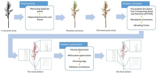
1. Introduction
- (1)
- We proposed a new aspect of skeleton optimization, which was named as the stump adjustment, and designed an algorithm for reconstructing the stump based on the layer and hierarchical relationship.
- (2)
- We proposed an algorithm for bifurcation optimization based on the local branch point cloud and cosine correlation.
- (3)
- After additionally adopting pruning twigs and Xu et al.’s [33] skeleton smoothness, we verified the differences between unoptimized skeletons and optimized skeletons and tested the optimized skeletons to extract some branch attributes and evaluate the accuracy.
2. Materials and Methods
2.1. Source and Preprocessing of Experimental Data
2.1.1. Data Source
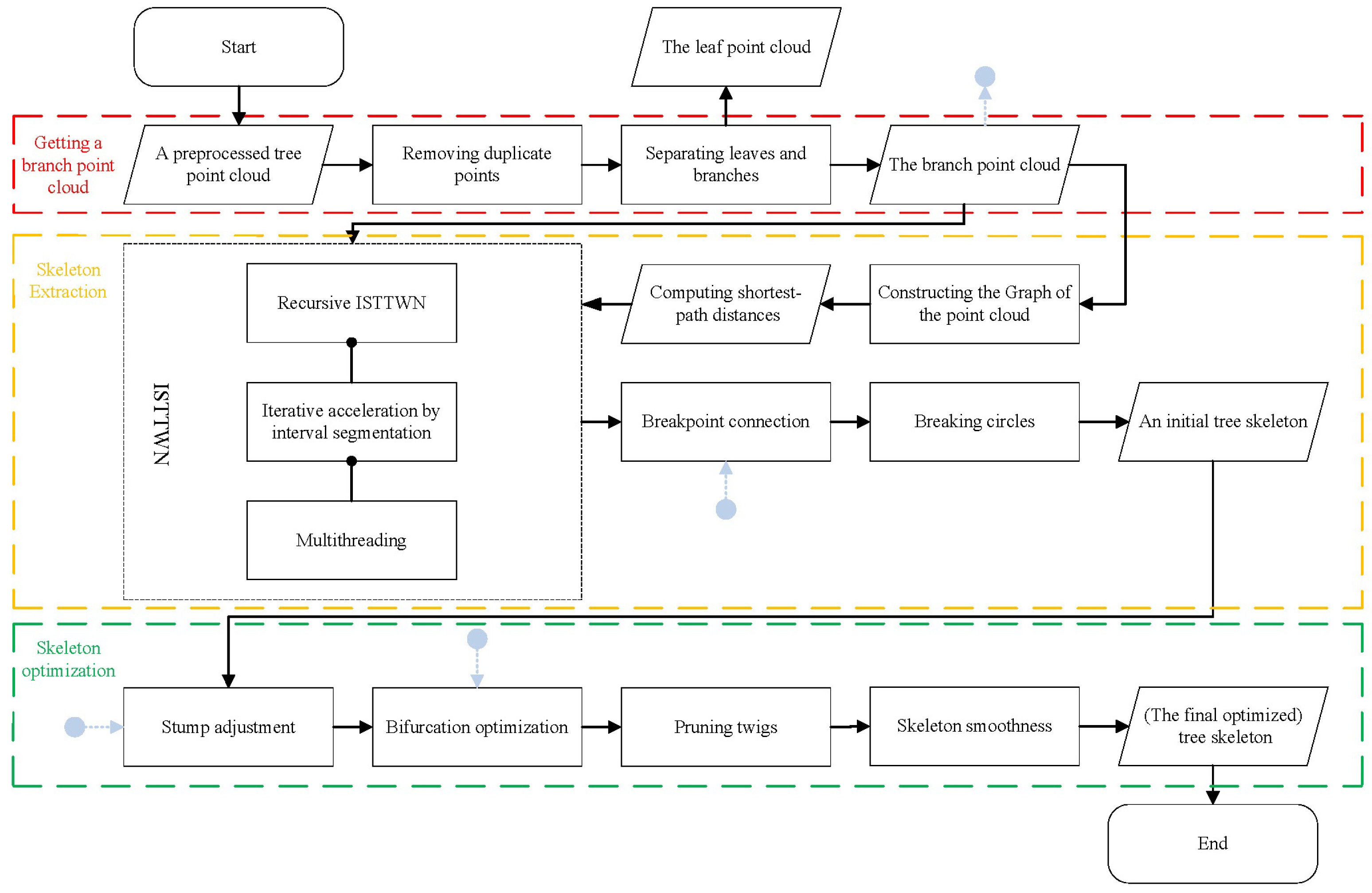
2.1.2. Separating Leaves and Branches
2.1.3. Computing the Shortest-Path Distances
2.2. Skeleton Extraction
- 1.
- Because skeleton lines are stored by ordered pairs, they can be regarded as directed edges in graph theory. Therefore, the indegree and outdegree of vertex corresponding to each skeleton point can be computed. Apart from the same vertex as the source vertex, any vertices where indegree is 0 are vertices corresponding to breakpoints.
- 2.
- For each breakpoint, use a kd-tree and k-Nearest-Neighbors (k-NN) search to find 3 neighbor points for which corresponding vertices are not on the tree, with the root being the vertex corresponding to the breakpoint. Compute the number of intersections between bin of breakpoints and bin of each neighbor point. We regarded that a neighbor point that the bin of which has the maximum number of intersections and the number is not equal to 0 should be the same point as the breakpoint. Then, the two points and their corresponding bin-s are required to be merged. If all numbers are equal to 0, directly connect the nearest one to the breakpoint.
2.3. Skeleton Optimization
2.3.1. Stump Adjustment
| Algorithm 1 Graph formed according to hierarchical relationship |
| Input: Skeleton point sequence , where is the size of skeleton point set; Bin sequence corresponding to each skeleton point in turn; Layer number sequence corresponding to each skeleton point in turn; Output: Undirected connected graph ;
|
- (1)
- The layer height is too large.
- (2)
- The tree species could be shrub.
- (3)
- The point cloud quality is bad.
- (4)
- Ground normalization has not been performed.
2.3.2. Bifurcation Optimization
2.3.3. Pruning Twigs
2.3.4. Skeleton Smoothness
3. Results
3.1. Computational Performance
3.2. Visual Analysis
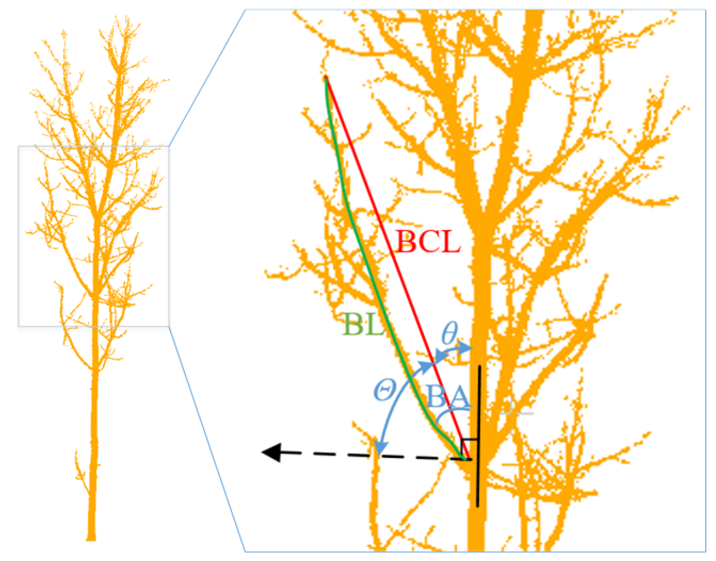
3.3. Application
4. Discussion
4.1. Quantitative Analysis and Comparison
4.2. Prospect
5. Conclusions
- (1)
- Different from the existing aspects of skeleton optimization, a stump adjustment is proposed according to the feature at the stump of the tree skeletons layering by the shortest-path distances. An algorithm for reconstructing the stump based on the layer and hierarchical relationship is designed correspondingly.
- (2)
- From the aspect of bifurcation optimization, an algorithm based on the local branch point cloud and cosine correlation is proposed.
- (3)
- Pruning twigs and Xu et al.’s [33] skeleton smoothness are adopted in the process of optimization.
Author Contributions
Funding
Data Availability Statement
Acknowledgments
Conflicts of Interest
References
- Guan, X. Research on the Modeling and Analysis of the Tree-dimensional Point Cloud Data of Trees. Master’s Thesis, Central South University of Forestry & Technology, Changsha, China, 2016. [Google Scholar]
- Sun, C.; Huang, C.; Zhang, H.; An, F.; Wang, L.; Yun, T. Individual Tree Crown Segmentation and Crown Width Extraction From a Heightmap Derived From Aerial Laser Scanning Data Using a Deep Learning Framework. Front. Plant Sci. 2022, 13, 914974. [Google Scholar] [CrossRef] [PubMed]
- Xue, X.; Jin, S.; An, F.; An, F.; Zhang, H.; Fan, J.; Eichhorn, M.P.; Jin, C.; Chen, B.; Jiang, L.; et al. Shortwave Radiation Calculation for Forest Plots Using Airborne LiDAR Data and Computer Graphics. Plant Phenomics. 2022, 2022, 9856739. [Google Scholar] [CrossRef] [PubMed]
- Wang, G.; Li, Q.; Yang, X.; Wang, C. Real Scene Modeling of Forest Based on Airborne LiDAR Data. J. Beijing Univ. Civ. Eng. Archit. 2021, 37, 39–46. [Google Scholar] [CrossRef]
- Li, Y.; Su, Y.; Zhao, X.; Yang, M.; Hu, T.; Zhang, J.; Liu, J.; Liu, M.; Guo, Q. Retrieval of tree branch architecture attributes from terrestrial laser scan data using a Laplacian algorithm. Agric. For. Meteorol. 2020, 284, 107874. [Google Scholar] [CrossRef]
- Ji, J. The broad-leaved tree leaves reconstruction and deformation based on laser-point-clouds. Master’s Thesis, Nanjing Forestry University, Nanjing, China, 2015. [Google Scholar]
- Huang, Z.; Huang, X.; Fan, J.; Eichhorn, M.; An, F.; Chen, B.; Cao, L.; Zhu, Z.; Yun, T. Retrieval of Aerodynamic Parameters in Rubber Tree Forests Based on the Computer Simulation Technique and Terrestrial Laser Scanning Data. Remote Sens. 2020, 12, 1318. [Google Scholar] [CrossRef]
- Shi, Y. 3D Simulation Theory and Technology of Botanic Tree Based on Scattered Point Cloud; Tongji University Press: Shanghai, China, 2018. [Google Scholar]
- Runions, A.; Lane, B.; Prusinkiewicz, P. Modeling Trees with a Space Colonization Algorithm. In Eurographics Workshop on Natural Phenomena; The Eurographics Association: Prague, Czech Republic, 2007. [Google Scholar] [CrossRef]
- Yang, H.; Wang, Y.; Wang, Z.; Zhang, Z. 3D Tree-modeling Approach Based on Competition over Space Resources. Comput. Sci. 2019, 46, 38–41. [Google Scholar]
- Zhang, Y.; Yu, W.; Zhao, X.; LYU, Y.; Feng, W.; Li, Z.; Hu, S. Interactive tree segmentation and modeling from ALS point clouds. J. Graph. 2021, 42, 599–607. [Google Scholar] [CrossRef]
- Hu, S.; Li, Z.; Zhang, Z.; He, D.; Wimmer, M. Efficient tree modeling from airborne LiDAR point clouds. Comput. Graph. 2017, 67, 1–13. [Google Scholar] [CrossRef]
- Zheng, J.; Fu, H.; Li, W.; Wu, W.; Yu, L.; Yuan, S.; Tao, W.Y.W.; Pang, T.K.; Kanniah, K.D. Growing status observation for oil palm trees using Unmanned Aerial Vehicle (UAV) images. ISPRS J. Photogramm. Remote Sens. 2021, 173, 95–121. [Google Scholar] [CrossRef]
- Zhou, C.; Yang, G.; Liang, D.; Yang, X.; Xu, B. An Integrated Skeleton Extraction and Pruning Method for Spatial Recognition of Maize Seedlings in MGV and UAV Remote Images. IEEE Trans. Geosci. Remote Sens. 2018, 56, 4618–4632. [Google Scholar] [CrossRef]
- Xu, H.; Gossett, N.; Chen, B. Knowledge and heuristic-based modeling of laser-scanned trees. ACM Trans. Graph. 2007, 26, 19. [Google Scholar] [CrossRef]
- Gao, S.; Zhang, H.; Liu, M.; He, Q.; Luo, L. Contour extraction of point cloud data for tree branches. J. Zhejiang A F Univ. 2013, 30, 648–654. [Google Scholar] [CrossRef]
- You. Stem Form Measurement Based on Point Cloud Data. Ph.D. Thesis, Chinese Academy of Forestry, Beijing, China, 2016. [Google Scholar]
- Raumonen, P.; Kaasalainen, M.; Åkerblom, M.; Kaasalainen, S.; Kaartinen, H.; Vastaranta, M.; Holopainen, M.; Disney, M.; Lewis, P. Fast Automatic Precision Tree Models from Terrestrial Laser Scanner Data. Remote Sens. 2013, 5, 491–520. [Google Scholar] [CrossRef]
- Li, G.; Liu, L.; Zheng, H.; Mitra, N. Analysis, Reconstruction and Manipulation using Arterial Snakes. ACM Trans. Graph. 2010, 29, 152. [Google Scholar] [CrossRef]
- Zhou, J. Research on Skeleton Extraction from Tree Point Cloud via k-Nearest-Neighbors-based Contraction. Master’s Thesis, Chongqing University, Chongqing, China, 2020. [Google Scholar]
- Sun, J.; Wang, P.; Li, R.; Zhou, M.; Wu, Y. Fast Tree Skeleton Extraction Using Voxel Thinning Based on Tree Point Cloud. Remote Sens. 2022, 14, 2558. [Google Scholar] [CrossRef]
- Zhang, Y.; Shen, B.; Wang, S.; Kong, D.; Yin, B. L0-regularization-based skeleton optimization from consecutive point sets of kinetic human body. ISPRS J. Photogramm. Remote Sens. 2018, 143, 124–133. [Google Scholar] [CrossRef]
- He, G.; Yang, J.; Behnke, S. Research on geometric features and point cloud properties for tree skeleton extraction. Pers. Ubiquitous Comput. 2018, 22, 903–910. [Google Scholar] [CrossRef]
- Livny, Y.; Yan, F.; Olson, M.; Chen, B.; Zhang, H.; El-Sana, J. Automatic Reconstruction of Tree Skeletal Structures from Point Clouds. ACM Trans. Graph. 2010, 29, 151. [Google Scholar] [CrossRef]
- He, L. Reseaches on 3D reconstruction of fruit tree’s trunk and its dynamic characteristics fo vibratory harvesting. Ph.D. Thesis, Zhejiang Sci-Tech University, Hangzhou, China, 2014. [Google Scholar]
- Wang, B. Studies on automatic 3D reconstruction techniques of trees based on terrestrial lidar point clouds. Master’s Thesis, Univerity of Electronic Science and Technology of China, Chengdu, China, 2015. [Google Scholar]
- Nouri, A.; Autrusseau, F.; Bourcier, R.; Gaignard, A.; l’Allinec, V.; Menguy, C.; Veziers, J.; Desal, H.; Loirand, G.; Redon, R. 3D bifurcations characterization for intra-cranial aneurysms prediction. In Proceedings of the Medical Imaging: Image Processing, San Diego, CA, USA, 19–21 February 2019. [Google Scholar] [CrossRef]
- Xu, J.; Shan, J.; Wang, G. Hierarchical Modeling of Street Trees Using Mobile Laser Scanning. Remote Sens. 2020, 12, 2321. [Google Scholar] [CrossRef]
- Fu, L.; Liu, J.; Zhou, J.; Zhang, M.; Lin, Y. Tree Skeletonization for Raw Point Cloud Exploiting Cylindrical Shape Prior. IEEE Access 2020, 8, 27327–27341. [Google Scholar] [CrossRef]
- Mei, J.; Zhang, L.; Wu, S.; Zhen, W.; Zhang, L. 3D tree modeling from incomplete point clouds via optimization and L1-MST. Int. J. Geogr. Inf. Sci. 2016, 31, 999–1021. [Google Scholar] [CrossRef]
- Li, R.; Bu, G.; Wang, P. An Automatic Tree Skeleton Extracting Method Based on Point Cloud of Terrestrial Laser Scanner. Int. J. Opt. 2017, 2017, 5408503. [Google Scholar] [CrossRef]
- Chaudhury, A.; Godin, C. Skeletonization of Plant Point Cloud Data Using Stochastic Optimization Framework. Front. Plant Sci. 2020, 11, 773. [Google Scholar] [CrossRef] [PubMed]
- Xu, S.; Li, X.; Yun, J.; Xu, S. An Effectively Dynamic Path Optimization Approach for the Tree Skeleton Extraction from Portable Laser Scanning Point Clouds. Remote Sens. 2022, 14, 94. [Google Scholar] [CrossRef]
- Yang, M.; Wu, E. Self-Adapting Algorithm of 3D Art-Designing Tree Skeleton Extraction. J. Front. Comput. Sci. Technol. 2012, 6, 1039–1048. [Google Scholar] [CrossRef]
- Li, J.; Wu, H.; Xiao, Z.; Lu, H. 3D modeling of laser-scanned trees based on skeleton refined extraction. Int. J. Appl. Earth Obs. Geoinf. 2022, 112, 102943. [Google Scholar] [CrossRef]
- Yang, J.; Wen, X.; Wang, Q.; Ye, J.S.; Zhang, Y.; Sun, Y. A Novel Algorithm Based on Geometric Characteristics for Tree Branch Skeleton Extraction from LiDAR Point Cloud. Forests 2022, 13, 1534. [Google Scholar] [CrossRef]
- Seidel, D.; Annighöfer, P.; Thielman, A.; Seifert, Q.; Thauer, J.H.; Glatthorn, J.; Ehbrecht, M.; Kneib, T.; Ammer, C. Predicting Tree Species From 3D Laser Scanning Point Clouds Using Deep Learning. Front. Plant Sci. 2021, 12, 635440. [Google Scholar] [CrossRef]
- Zhang, D.; Yan, R.; Yun, T.; Xue, L.; Ruan, H. The 3D reconstruction of tree branches from point cloud based on terrestrial laser scanner. J. For. Eng. 2016, 1, 107–114. [Google Scholar] [CrossRef]
- Zhao, Y.; Guo, H. A Tree Branch Skeleton Extraction Approach Based on Point Cloud. Comput. Digit. Eng. 2016, 44, 1333–1337. [Google Scholar] [CrossRef]
- Thurlbeck, A.; Horsfield, K. Branching angles in the bronchial tree related to order of branching. Respir. Physiol. 1980, 41, 173–181. [Google Scholar] [CrossRef] [PubMed]
- Uylings, H. Optimization of diameters and bifurcation angles in lung and vascular tree structures. Bull. Math. Biol. 1977, 39, 509–520. [Google Scholar] [CrossRef] [PubMed]
- King, D.; Loucks, O.L. The theory of tree bole and branch form. Radiat. Environ. Biophys. 1978, 15, 141–165. [Google Scholar] [CrossRef] [PubMed]
- Harper, G.J. Quantifying branch, crown and bole development in Populus tremuloides Michx. from north-eastern British Columbia. For. Ecol. Manag. 2008, 255, 2286–2296. [Google Scholar] [CrossRef]
- Dong, L.; Liu, Z.; Bettinger, P. Nonlinear mixed-effects branch diameter and length models for natural Dahurian larch (Larix gmelini) forest in northeast China. Trees 2016, 30, 1191–1206. [Google Scholar] [CrossRef]
- Du, S.; Lindenbergh, R.; Ledoux, H.; Stoter, J.; Nan, L. AdTree: Accurate, Detailed, and Automatic Modelling of Laser-Scanned Trees. Remote Sens. 2019, 11, 2074. [Google Scholar] [CrossRef]
- Ai, M.; Yao, Y.; Hu, Q.; Wang, Y.; Wang, W. An Automatic Tree Skeleton Extraction Approach Based on Multi-View Slicing Using Terrestrial LiDAR Scans Data. Remote Sens. 2020, 12, 3824. [Google Scholar] [CrossRef]
- Wu, B.; Zheng, G.; Chen, Y.; Yu, D. Assessing inclination angles of tree branches from terrestrial laser scan data using a skeleton extraction method. Int. J. Appl. Earth Obs. Geoinf. 2021, 104, 102589. [Google Scholar] [CrossRef]
- Fan, G.; Nan, L.; Dong, Y.; Su, X.; Chen, F. AdQSM: A New Method for Estimating Above-Ground Biomass from TLS Point Clouds. Remote Sens. 2020, 12, 3089. [Google Scholar] [CrossRef]
- Huang, Z. Tree skeleton reconstruction and wind resistance analysis based on laser point cloud. Master’s Thesis, Nanjing Forestry University, Nanjing, China, 2020. [Google Scholar] [CrossRef]


| Tree Species | Size of Original Tree Point Cloud | Number of Duplicate Points | Size of Branch/Leaf Point Cloud | of Branch Point Cloud | Number of Edges in Constructed Undirected Graph | |
|---|---|---|---|---|---|---|
| European ash | 97,895 | 0 | 0.016659 m | 94,021/3874 | 0.166197 m | 14,582,170 |
| European oak | 836,636 | 4 | 0.005627 m | 819,556/17,076 | 0.056221 m | 164,547,719 |
| American black poplar | 565,698 | 288,680 | 0.011883 m | 274,688/2330 | 0.118744 m | 70,006,006 |
| Tree Species | ISTTWN | Stump Adjustment | Bifurcation Optimization | Pruning Twigs | Skeleton Smoothness |
|---|---|---|---|---|---|
| European ash | 244 | 138 | 183 | 67 | 67 |
| European oak | 1036 | 518 | 674 | 257 | 257 |
| American black poplar | 705 | 508 | 731 | 268 | 268 |
| Evaluation Indexes | BA | BCL | BL | |
|---|---|---|---|---|
| 0.164641 () | 0.086456 () | 0.203494 m | 0.192263 m | |
| 0.124162 () | 0.061605 () | 0.129652 m | 0.125959 m | |
| 13.513% | 9.4927% | 5.6421% | 6.9631% | |
| 0.684622 | 0.896877 | 0.986168 | 0.988428 |
Publisher’s Note: MDPI stays neutral with regard to jurisdictional claims in published maps and institutional affiliations. |
© 2022 by the authors. Licensee MDPI, Basel, Switzerland. This article is an open access article distributed under the terms and conditions of the Creative Commons Attribution (CC BY) license (https://creativecommons.org/licenses/by/4.0/).
Share and Cite
Yang, J.; Wen, X.; Wang, Q.; Ye, J.-S.; Zhang, Y.; Sun, Y. A Novel Scheme about Skeleton Optimization Designed for ISTTWN Algorithm. Remote Sens. 2022, 14, 6097. https://doi.org/10.3390/rs14236097
Yang J, Wen X, Wang Q, Ye J-S, Zhang Y, Sun Y. A Novel Scheme about Skeleton Optimization Designed for ISTTWN Algorithm. Remote Sensing. 2022; 14(23):6097. https://doi.org/10.3390/rs14236097
Chicago/Turabian StyleYang, Jie, Xiaorong Wen, Qiulai Wang, Jin-Sheng Ye, Yanli Zhang, and Yuan Sun. 2022. "A Novel Scheme about Skeleton Optimization Designed for ISTTWN Algorithm" Remote Sensing 14, no. 23: 6097. https://doi.org/10.3390/rs14236097
APA StyleYang, J., Wen, X., Wang, Q., Ye, J.-S., Zhang, Y., & Sun, Y. (2022). A Novel Scheme about Skeleton Optimization Designed for ISTTWN Algorithm. Remote Sensing, 14(23), 6097. https://doi.org/10.3390/rs14236097