Article

Automatic Detection of Marine Litter: A General Framework to Leverage Synthetic Data

1
Mines Paris—PSL Research University, 60 Boulevard Saint Michel, 75005 Paris, France
2
C.R.C. Centre of Research on Risks and Crisis, MINES Paris, PSL Research University, 1 rue Claude Daunesse, 06560 Sophia Antipolis, France
3
“Politehnica” University of Bucarest, UPB, Splaiul Independentei 313, 060042 Bucarest, Romania
4
O.I.E. Centre Observation, Impacts, Energy, MINES Paris, PSL Research University, 1 rue Claude Daunesse, 06560 Sophia Antipolis, France
*
Author to whom correspondence should be addressed.
Remote Sens. 2022, 14(23), 6102; https://doi.org/10.3390/rs14236102
Submission received: 6 October 2022 / Revised: 18 November 2022 / Accepted: 28 November 2022 / Published: 1 December 2022

Abstract

:
The spatial and temporal coverage of spaceborne optical imaging systems are well suited for automated marine litter monitoring. However, developing machine learning-based detection and identification algorithms requires large amounts of data. Indeed, when it comes to marine debris, ground validated data is scarce. In this study, we propose a general methodology that leverages synthetic data in order to avoid overfitting and generalizes well. The idea is to utilize realistic models of spaceborne optical image acquisition and marine litter to generate large amounts of data to train the machine learning algorithms. These can then be used to detect marine pollution automatically on real satellite images. The main contribution of our study is showing that algorithms trained on simulated data can be successfully transferred to real-life situations. We present the general components of our framework, our modeling of satellites and marine debris and a proof of concept implementation for macro-plastic detection with Sentinel-2 images. In this case study, we generated a large dataset (more than 16,000 pixels of marine debris) composed of seawater, plastic, and wood and trained a Random Forest classifier on it. This classifier, when tested on real satellite images, successfully discriminates marine litter from seawater, thus proving the effectiveness of our approach and paving the way for machine learning-based marine litter detection with even more representative simulation models.

Graphical Abstract

1. Introduction

1.1. Background

Being able to detect large patches of floating debris, such as macro-plastics, in coastal waters will help better understand the sources, pathways, and trends that lead to this type of pollution. Although remote sensing for plastic detection is still in its infancy, there is an increasing number of papers providing promising results on plastic detection over water as well as on land [1,2,3,4,5]. In particular, satellites, being designed to provide observations of global scope, continuous temporal coverage, and harmonized data collection and processing, could be ideal tools for global marine debris monitoring [6]. However, there is a need for complementary in situ measurements which, combined with remote sensing observations, allow for calibration and validation of data from the satellites. In this vein, Maximenko et al. [5] are developing the Integrated Marine Debris Observing System (IMDOS).
Among recent studies on the matter, many have used optical data from Sentinel-2 (S2), a satellite constellation developed by ESA (the European Space Agency). Launched in 2015, they have a 13-band multispectral instrument (MSI) sensor and they collect data with a Ground Sampling Distance (GSD) of 10 m , 20 m , or 60 m , depending on the band. The data are openly-accessible and the revisit time is 10 days at the equator with one satellite, and 5 days with two satellites (Sentinel 2A and 2B). Coveragewise, it includes all continental land surfaces, all coastal waters up to 20 km from the shore and all closed seas such as the Mediterranean [7]. All these features make it an interesting tool for the detection of floating plastics in coastal waters compared to most of the available sensors which provide images that either have a poor resolution, a low revisit time or are not freely and openly distributed.
A first requirement to detect plastic using satellites such as S2 is to collect data that we know contains plastic. This first step, though it seems basic, is quite challenging since it requires ground validation. Out of the studies that have been conducted, two trends have emerged regarding this matter, while Biermann et al. [8] and Kikaki et al. [9] rely on ground truth events reported by citizen scientists, media, and social media, Topouzelis et al. [10] and Themistocleous et al. [11] rely on controlled in situ validation. In 2018, Topouzelis et al. [10] have developed large 10   m × 10   m artificial plastic targets and deployed them in the Aegean sea. They collected spectral data of these targets both from S2 and Unmanned Aerial Vehicles (UAV). These campaigns, collectively called the Plastic Litter Projects (PLP) have been conducted each year since 2018. They have provided the first in situ estimates of the spectral signatures of floating macro-plastics [10,12]. This work inspired Themistocleous et al. [11] to deploy their own plastic target on the coast of Cyprus and thus to collect more in situ data.
The large sizes considered for these targets are motivated by the resolution of the satellite: the S2 bands with the best resolution have a GSD of 10 m. Although these large patches are not necessarily representative of floating plastics in the open ocean, these controlled experiments provide exact descriptions of constituents as well as locations and dates of the patches, thus enabling a reliable collection of data. This method ensures a higher degree of certainty than relying on third-party reporting, as in [8,9].
Another data source that has become more and more used in recent years is data from UAVs. For example, Goddijn-Murphy et al. [13] have used UAVs equipped with Thermal Infrared (TIR) cameras to detect floating macro plastics. They also showed how TIR data can be used to supplement data acquired in the visible and short-wave infrared ranges.
UAVs have also been successfully used to detect debris on beaches [14,15], rivers [16,17], and to track the evolution of debris patches [18]. For more details about the use of UAVs in marine remote sensing, see the review by Yang et al. [19].
There are clear advantages to using data sourced from UAVs, namely, the high spatial resolution that can be obtained, the flexibility of the acquisition and the relatively low economic impact of running a collection campaign. However, they lack the global coverage that satellites can provide. This is of utmost importance if we are looking to detect previously-unknown debris locations.

1.2. Issues

Among the recent studies on the use of satellites to detect plastic, many mention the development of automated marine debris detection algorithms based on machine learning. As mentioned, the main obstacle for this is the lack of data: ground-truth validation of satellite data containing plastic pixels is scarce. The work of Topouzelis et al. [10] and Themistocleous et al. [11] has been instrumental in collecting this kind of validated data. Moreover, the same data have to be used for both training and testing. Thus, the risk of overfitting and poor generalization is high. As a consequence, the algorithms developed for automated plastic detection are unlikely to be robust enough for operational use. Biermann et al. [8] have trained a Naïve Bayes classifier on 53 plastic pixels collected from the same image in Durban, 20 seawater pixels, and a few other pixels for other marine debris. Basu et al. [20] have created a dataset composed of pixels of plastic extracted from the experiments in [10,11], but in quantities close to those in [8]: 59 plastic pixels for 458 seawater pixels.
As a follow-up to the previous work, Sannigrahi et al. [21] investigated the performance of several machine learning algorithms on a larger datasets (234 plastic pixels and 234 water pixels for the largest one). Similarly, Taggio et al. [22] have implemented machine learning algorithms trained on pixels acquired from the same targets, but using a different satellite, PRISMA. This particular satellite has a higher resolution than S2 on the panchromatic band and significantly more spectral bands. They trained their algorithms on a pan-sharpened version of the PRISMA images.
Even though all of the previously mentioned works obtained satisfying accuracies on plastic pixels, these promising results may be questionable in terms of generalization capability, as the amount of data used for training and testing is low. For instance, it is well known that a Naïve Bayes classifier may approximate a conditional distribution under the (rather strong) hypothesis of conditional independence. However, without this assumption, the estimate with Bayes’ rule of P ( y | x ) , with y being, for instance, the fact that a pixel contains plastic or not and x a b-dimensional vector of n-ary features, i.e., the b spectral bands, each taking one of n discrete possible values, would require several training sets with at least 2 ( n b 1 ) samples each. Clearly, in operationally-relevant cases, n must be large, thus requiring a high number of samples for training. With more complex machine learning models, such as neural networks, the requirement on the number of training samples is more stringent [23].
At the same time, increasing the number of plastic pixels with ground-truth validation presents challenges when it comes to rapidly iterating on machine learning algorithms, since developing measurement campaigns is expensive and time-consuming. This problem is not inherent to remote sensing in general, for instance Cao and Huang [24] tackle the challenge of detecting Green Plastic Cover (GPC) used for covering construction sites. In their case, their dataset contains more than 50,000 samples with 5000 of them containing GPC samples. However, as presented earlier, such amount of validated samples does not exist in our problem domain.
Knaeps et al. [25] have recently provided hyperspectral reflectance measurements of plastic samples in a controlled environment, simulating clear to turbid waters. This type of work paves the way for developing simulations.

1.3. Leveraging Synthetic Data

In line with recent trends of using data augmentation techniques to train more robust machine learning algorithms when data collection is costly (for example [26,27]), we investigated the possibility of generating synthetic data to train machine learning algorithms that usually perform well in operating conditions.
Synthetic data is data that is generated on a computer by an algorithm, as opposed to captured by a sensor. This type of data can have various purposes. For example, in a remote-sensing context, Tournadre et al. [28] simulate the reflectance of the top of the atmosphere in clear-sky conditions. Their goal is to then use these simulations, together with real data to estimate cloud coverage. Hoeser and Kuenzer [29] generate synthetic data to train machine learning algorithms to detect offshore wind farms from Sentinel-1. They choose to go down this path after identifying the same main issue as us, namely the scarcity of well-validated data. They develop an ontology approach to generate random images based on expert knowledge. Kong et al. [30] use a 3D urban environment modeling system to generate synthetic Sentinel-1 images to train machine learning algorithms for building segmentation. We take a different perspective based on the direct simulation of selected characteristics of the physical object that constitutes an image.
The main goal of our study is to showcase a proof of concept of the transferability of marine debris detection from synthetic data to real data. We propose a general methodology that includes a physical model of debris patches at sea and of satellite data acquisition. We implemented this model into a simulator that can generate large datasets of synthetic images. These are then used to train algorithms that learn to discriminate debris and water. We illustrate this method with a case study of macro-plastic detection from S2 with validation on existing S2 images provided by the PLP.

1.4. Structure of the Paper

Section 2 presents our methodology and the case study on S2. More particularly, in Section 2.1, we introduce the various models that are used to generate the synthetic data. Then, Section 2.2 shows how these models are used to simulate S2 images. We begin this section by presenting the data sources for our case study. Following is a more in-depth description of the dataset generation process. The same section also investigates how aliasing artifacts affect S2 images and proposes a method for reproducing similar artifacts in our own simulation.
Afterwards, Section 3 presents and analyses the results of a classifier trained on simulated images on in situ validated data.
Section 4 discusses the advantages and shortcomings of our methodology and proposes future study directions. Finally, in Section 5, we conclude the study with a summary of our work and results.

2. Materials and Methods

2.1. Methodology and Modelling

2.1.1. Methodology Outline

Figure 1 presents the proposed methodology. The goal is to overcome the lack of data when it comes to marine litter detection from satellites. The solution proposed is to model a simple spaceborne optical image acquisition system for seawater and marine debris, to generate synthetic data that encapsulate the challenges and particularities of real marine debris.
Once these data are generated in large amounts, it is possible to train, validate and test classifiers. The final classifier can be checked on real images, acquired for this purpose with ground-truth validation.

2.1.2. Optical Modeling

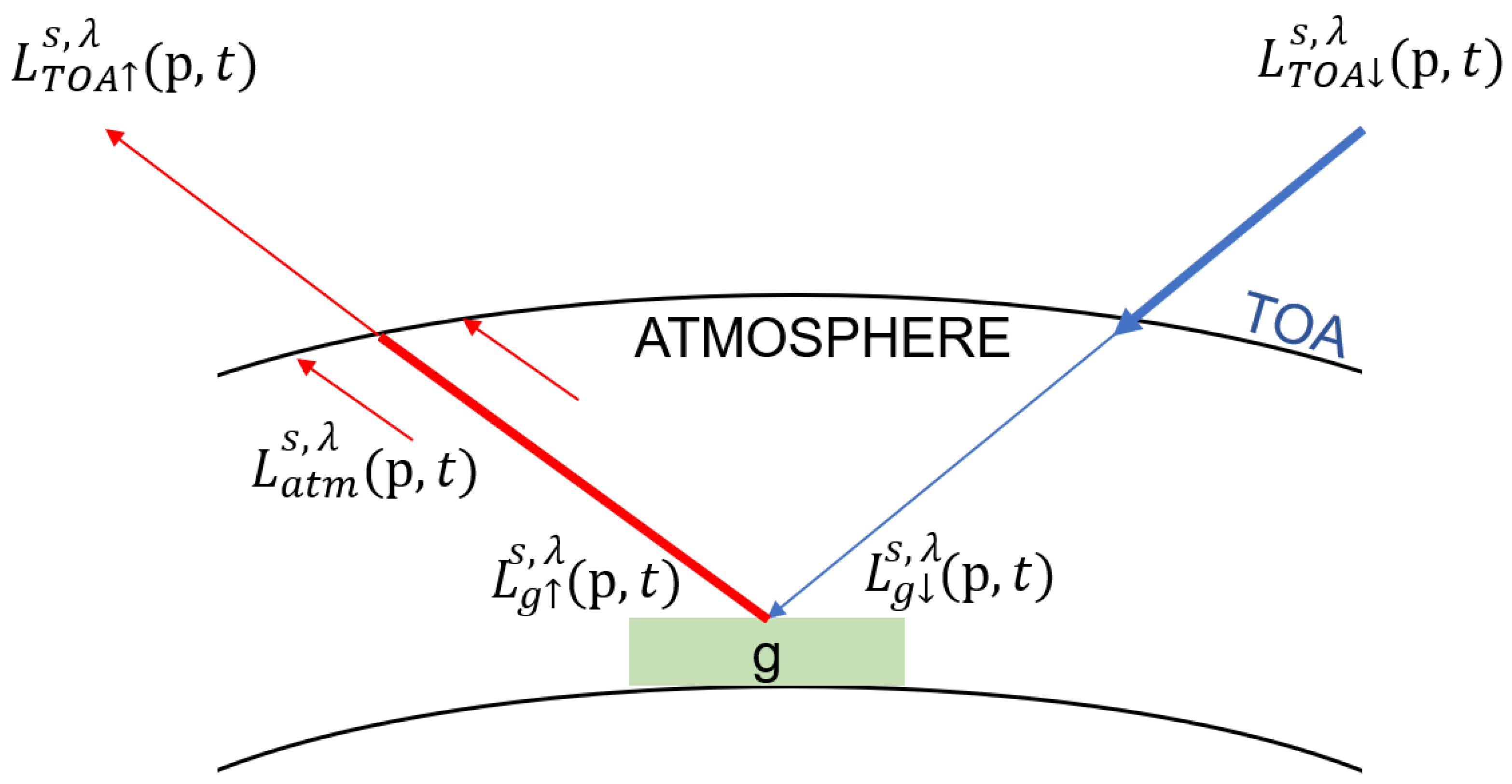
For a visual illustration of the quantities used in the optical model, see Figure 2.
From an optical point of view, satellite acquisition process may be modeled as a spatial filter for each wavelength [31]. Neglecting the radiative sources that are predominant for wavelengths greater than 2.5   μ m , the radiance received by the satellite sensors is, for each spectral band s and wavelength λ s :
L S A T s , λ p , t = Ω psf s u L T O A s , λ p u , t d u
where Ω is the surface of the detector, p is the position on the surface of the detector of a point g, observed on the surface of the Earth; t represents the picture acquisition time. Moreover:
  • psf s is the Point Spread Function for band s. It defines the local response of a Dirac delta impulse in the resulting image [32]. It is thus the convolution kernel of the filter.
  • L T O A s , λ p , t = τ a t m s , λ p , t L g s , λ p , t + L a t m s , λ p , t is the ascending top of the atmosphere radiance, with τ a t m s , λ being the atmospheric transmittance and L a t m s , λ being the atmosphere in-scattering term. All these terms are defined for each band.
  • L g s , λ p , t = ρ g λ p L g s , λ p , t where ρ g λ p is the reflectance of the object on the ground, and L g s , λ p , t sums the flux of light received by the object from the sun taking into account all atmospheric effects.
To simplify the model, we consider the following hypotheses:
  • H1: All the terms are constant in time when compared to the timescale of image acquisition.
  • H2: The observed scene is considered small enough so that τ a t m s , λ and L a t m s , λ are constant with respect to p, i.e., the atmosphere is assumed to be the same in a neighborhood.
  • H3: To simplify further, the effects of the atmosphere are neglected. The term L a t m is overlooked and τ a t m is set to 1. This is in accordance with real satellite images corrected of the effect of the atmosphere, as they are made available by ESA, supposing that this correction is perfect.
  • H4: Keeping in mind our disregard of the atmosphere, we have: L g s , λ p L T O A s , λ p . This implies that L T O A s , λ p ρ g λ p L T O A s , λ p .
  • H5: L T O A s , λ p = I 0 λ r E S 2 , the descending top of the atmosphere radiance, is considered constant for band s. I 0 is the solar constant and r E S the distance between the earth and sun. With this, we ignore the geometric parameters of the sun and satellite.
While these hypotheses are certainly only approximations of the real conditions, our aim is not to obtain the best possible satellite model, but a proof of concept of the transferability of a classifier. Under these hypotheses, the radiance received by the detector for a given band is:
L S A T s p = s S s ( λ ) psf s * ρ g λ p L T O A s d λ
where S s ( λ ) is the spectral sensitivity of band s and * is the convolution described in Equation (1). We consider that S s ( λ ) integrates to 1. If that is not the case, a normalization step is also required.
In addition, we consider the internal noise of the measuring system:
  • H6: The noise N ( p ) follows a normal law N ( μ , σ 2 ) , with μ being the mean and σ 2 the variance.
For large values of σ , this noise can summarize the approximation of the overlooked terms.
The signature of marine debris is usually expressed in terms of reflectance. To go from our radiance model to a reflectance model, we need only divide all terms by the constant term L T O A s .
Putting all of this together, the final equation of reflectance for band s becomes:
ρ S A T s p = N ( p ) + s S s ( λ ) p s f s * ρ g s p d λ

2.1.3. Sampling Modelling

Once the landscape has been acquired by the different optical sensors of the system, the corresponding image in the focal plane is spatially discretized over a given integration time (pose) by the CMOS detectors into a digital image. Among all the steps, modeling the sampling process is critical to ensure the reliability of the data given the scale of the target. Depending on the GSD, aliasing might introduce distortion or artifacts on the reconstructed signal, in addition to the noise. According to the Nyquist–Shannon sampling theorem, the sampling process is reversible if the sampling frequency of a signal, f s , is at least double the frequency of its highest frequency component [33]. If f c is the cut-off frequency of a signal, i.e., the inverse of the smallest dimension that the optical apparatus can discriminate, the theorem can be written as:
f s > 2 f c 1 2 GSD > f c
1 / ( 2 GSD ) being the Nyquist frequency, f n .
In the case of an optical imaging system, the value of the spatial cut-off frequency is calculated as follows:
f c D λ H
with D being the diameter of the pupil in meters, λ the wavelength of the band in meters, and H the altitude of the satellite in meters.
For instance, in the case of S2, the diameter of the pupil is 150 m m , the altitude of the satellite is 786 k m , and the wavelength depends on the spectral band [7]. Table 1 shows the values of the cut-off and Nyquist frequencies for each band.
As highlighted by Table 1, the f c f n ratio is always superior to 1, meaning the the Shannon–Nyquist theorem is never verified. If we consider B02, which has the best spatial resolution and the shortest wavelength, respecting the Shannon–Nyquist condition without modifying the characteristics of the satellite (diameter of the pupil, altitude of the satellite) would imply having a GSD about 10 times smaller.
Thus, the choice of design of S2, which privileged a large pupil diameter to enhance the contrast and improve the Signal to Noise Ratio (SNR), induces some potentially strong aliasing effects that the end-user must be aware of, especially when the size of the elements of interest are close to the GSD. Similar phenomena have been observed to have a strong impact on other satellites, such as SPOT [31].
For a simulation to be correct and take into account all the effects introduced by aliasing, we must consider the situation where the Shannon–Nyquist is not respected by the satellite we are modeling. In such a situation, we need to simulate the landscape at a resolution compatible with the maximum cut-off frequency of the satellite. By generating the landscape at a resolution where the Shannon–Nyquist theorem is respected and then resampling it with the same GSD as the satellite, we can faithfully reproduce the aliasing artifacts that would be observable in real images. To determine a suitable pixel size for the landscape generation, we propose the following method:
  • Calculate the GSD under which no detail can be perceived by the optical system: GSD m i n = 1 2 max ( f c ) .
  • Based on the actual GSDs of the satellite bands, find a number, d, that evenly divides into all of them and that is smaller than GSD m i n .
  • When building the initial image, before any other processing, consider a pixel to be a square of size d × d .
In order to model the relative position of the satellite with the target, we consider the target as fixed at the center of the image, and the grid of sensors (evenly spaced spaced by the GSD of the band under consideration) is regarded as rigidly moving with sub-pixel translations, thus accounting for geometric uncertainty and inherent variability, module one pixel, from one acquisition to another. These rigid geometric shifts are hereinafter named jitters. This is equivalent to selecting pixels, evenly spaced in both directions by the GSD, starting from a random offset i , j drawn between GSD / 2 and GSD / 2 . See Section 2.2 for an example of an implementation with S2.

2.1.4. Marine Debris and Seawater Model

In the ocean, natural and anthropogenic materials tend to be aggregated together and to form patches of mixed objects, including macro-plastics [20]. Once aggregated into sufficiently large patches of varying shapes and sizes, the detection from satellites becomes possible.
In our model, we consider patches made out of marine debris material. To generate the patches, we take into account the following:
  • The shape: in this proof of concept, the patch can either be a rectangle or a circle. These simple shapes are consistent with the targets used by [10].
  • The size: if it is a rectangle, two dimensions are required for the length and the width whereas if it is a circle, only the radius is required.
  • The type of material: can be specified among a list of predefined material types. Based on the material, the corresponding reflectance values are loaded from a database of spectral reflectance values.
  • The fraction of material: a number between 0 and 1 which defines the proportion of material contained in the patch. If the value is 0, there is only seawater and if the value is 1, the patch is 100% filled by the material. This parameter is used as an attenuation factor to model patches where the material does not completely cover the water (as a cover percentage) or to model other types of attenuation such as biofouling. Furthermore, it can be used to weaken the amplitude of the spectral reflectance that are measured in conditions too far from reality. Within a patch, the same attenuation is applied to each pixel.
  • The rotation: a number in the [−45°, 45°] range that defines the rotation of the patch. In real conditions, the material patch might not be aligned with the pixels. This is only applied when the shape is a rectangle.
  • The bands: the interval of wavelengths of the bands considered for the satellite.
As for seawater, it typically has a low reflectance, except in cases of sun glint (due to specular effects). As we do not take into account geometrical and lighting parameters in this first proof of concept, we chose to model all of the seawater pixels the same way by loading a default seawater spectral signature (see Section 2.2.1). This simplistic model does not take into account particularities such as turbid water or specular conditions.

2.1.5. Dataset Generation

The models presented above can be used, by changing various parameters, to generate synthetic data in large quantities. Given large datasets, more robust machine learning algorithms can be developed and trained, with specific datasets dedicated to validation. Indeed, the large amount of data makes it possible to split them between train, validation and test sets in order to avoid overfitting while adjusting the hyperparameters of the machine learning model. Note that these validation and test sets are independent of the ground truth validation set (i.e., the data from the PLP, in our case), which are used only at the final stage.

2.2. Case Study on Sentinel-2

Here we describe the application of our framework to generate a large dataset based on S2 features.

2.2.1. Data Sources

The spectral signatures of the different types of plastic have been collected from [25]. They provide a dataset of 47 hyperspectral reflectance measurements of plastic litter samples in different conditions: dry, wet, submerged at different depths, and with varying suspended sediment concentrations. Measurements of the spectral reflectance were performed in an optical calibration laboratory and in a water tank and were analyzed in a study conducted by [34]. We extracted plastic materials (plastic bags, plastic bottles, placemats, etc.) and also wood from this dataset. We chose varying conditions: some of the materials are dry while others are wet or submerged (depth from 0 cm to 4 cm). When several colors were available (for placemats for instance), we selected all of them. The data is in open-access and are made available by [25].
The spectral signature of seawater has been collected from the Sentinel-2 USGS Spectral library v.7 using the seawater signature for coastal waters [35]. The data is available at [36].
The spectral sensitivity ( S s ( λ ) in Equation (1)) can be downloaded at [37]. Finally, the psf s for all of the S2 spectral bands are available at [38] (which also contains the source code of the simulator). The PSFs have been computed knowing the diameter of the pupil, the focal length, the different spectral sensitivity of the 13 bands, and using standard values for MTF due to detectors and satellite orbit, following Section 3.4 of [32].

2.2.2. Processing Steps

As described in Section 2.1.3, the maximum cut-off frequency of S2 is for B01 with a value of f c = 0.43 m 1 . Hence, GSD m i n = 1 2 · 0.43 = 1.16 m. Given that 1 m (≤1.16 m) divides evenly into all the GSDs of all the S2 bands, we chose this value for d. Each pixel in the initial image represents a 1   m × 1   m square. The scene is made of an image of size 540 × 540 pixels with the patch at the center. The pixels of the patch are filled with the configured material’s reflectance values, taken from its spectral signature, while the other pixels are filled with the reflectance values of seawater. Out of one scene, 13 simulated images are generated, one for each of the 13 bands of S2, taking into consideration the characteristics of each band.
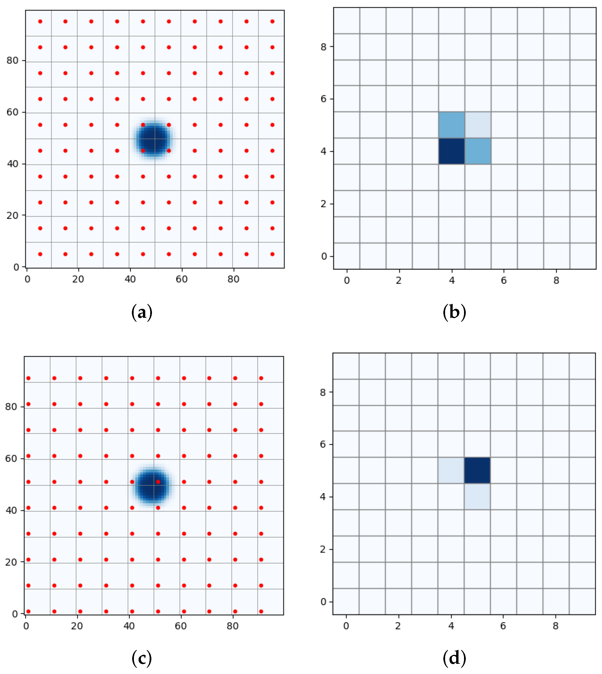
Each of the 13 simulated images from the same scene is convolved with the PSF corresponding to the band. The resulting convolution is then re-sampled so it conforms to the GSD of the band (e.g., 60 m for B01 or 10 m for B02). Figure 3a shows the result of the convolution between a scene with a circular plastic patch and the PSF of band B02–whose GSD is 10 m . The plastic is in dark blue and the seawater in the background is white. The values of the pixels are reflectance values corresponding to plastic and seawater.
The image is then sampled (see Section 2.1.3). Figure 3b shows the resulting image for a specific jitter. As can be seen in Figure 3c,d, a different jitter leads to dramatically different results.
Optionally, once the 13 simulated images are convolved and sampled, noise can be added on each image based on the model presented in Section 2.1.2. We specialized the normal law as N ( 0 , σ 2 ) , with σ being one of the following values: 0.01, 0.02, 0.05, 0.1. The standard deviations have been chosen for sensitivity analysis and do not correspond to the SNR of S2.
The output of the simulation is a package of 13 processed image and a binary mask that marks which pixels are part of the patch. Figure 4 illustrates the process, as described in the previous paragraphs.

2.2.3. Assessment of the Simulation Performance

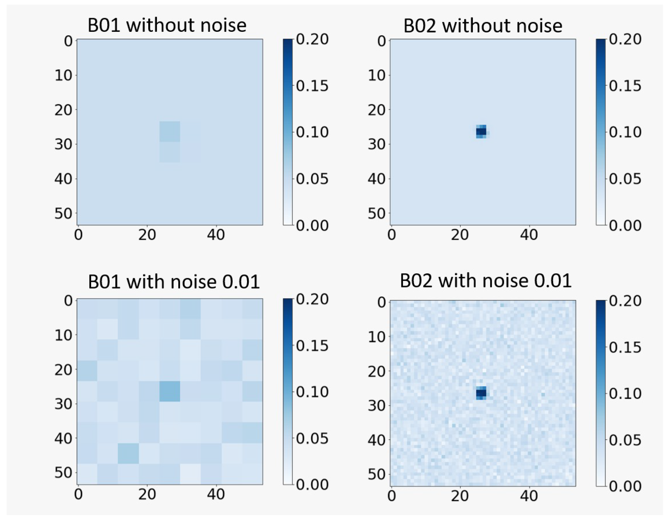
Figure 5 shows the output obtained by the simulation for the following inputs with a random jitter (constant across the entire image and all bands). For visibility purposes, only band B01 and B02 are displayed.
  • Shape: rectangle;
  • Size: 30   m × 30   m ;
  • Type of plastic: wet bottles frame;
  • Rotation: 10°;
  • Fraction of plastic: 1;
  • Noise level: 0.01.
It is easy to identify the bands with the best spatial resolution and the worst ones. Band B01 has a GSD of 60 m, the plastic pixels are barely recognizable on a seawater background without noise and with a noise with σ = 0.01 , the plastic is no longer detectable. This observation also applies for bands B09 and B10. The bands with a GSD of 10 m (B02, B03, B04, and B08) are better suited for plastic detection with a sharp noticeable signal, even in the presence of noise.
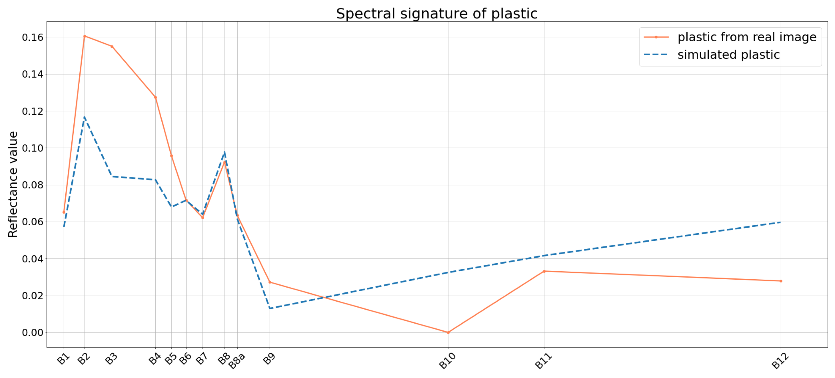
Figure 6 shows the spectral signature of both the plastic simulated with the inputs mentioned above and the plastic collected from an Level 2A S2 image acquired on 11 June 2021 over the Gulf of Gera on the island of Lesvos, Greece. The PLP team deployed a circular target of 28 m diameter made out of HDPE (high-density polyethylene) mesh for the PLP21 [39] and we collected the plastic spectral signature from this target. The fraction of plastic for the simulated image was set to 0.6 to match the fraction of plastic of the HDPE mesh, and the noise was set to 0.01. The reflectance values of the spectral signature are different in the visible range, particularly for B02, B03, B04 and B05. The reasons of these discrepancies could be that the materials are not exactly the same. More particularly, the colors are different: the HDPE mesh is white whereas the bottles frame material are supposedly transparent, explaining the lower reflectance values. All things considered, the results are satisfying and close to in situ measurements. However, as the noise level increases, the discrepancies increase as well and the spectral signature is less recognizable. For a noise with σ = 0.02, the results are not far from the ones at 0.01, but when it comes to a noise level of 0.1, the results are less satisfying.

2.2.4. Aliasing Artifacts in Sentinel-2 Data

Beyond illustrating the sampling process, Figure 3 also showcases the reproduction of the aliasing effect occurring in the S2 sampling process. Within the same cell, several jitters can be chosen (100 possible jitters for a band with GSD = 10 m). Depending on the jitter, the final value is not the same. In Figure 3b,d, it is possible to see that the final result will be different if the jitter is 5 , 5 or 1 , 1 . Therefore, depending on the jitter, the value can be drastically different. This is how the loss of information or artifacts occur in the S2 sampling process. By generating different scenes in different conditions, we can investigate the range of sizes sensitive to aliasing.
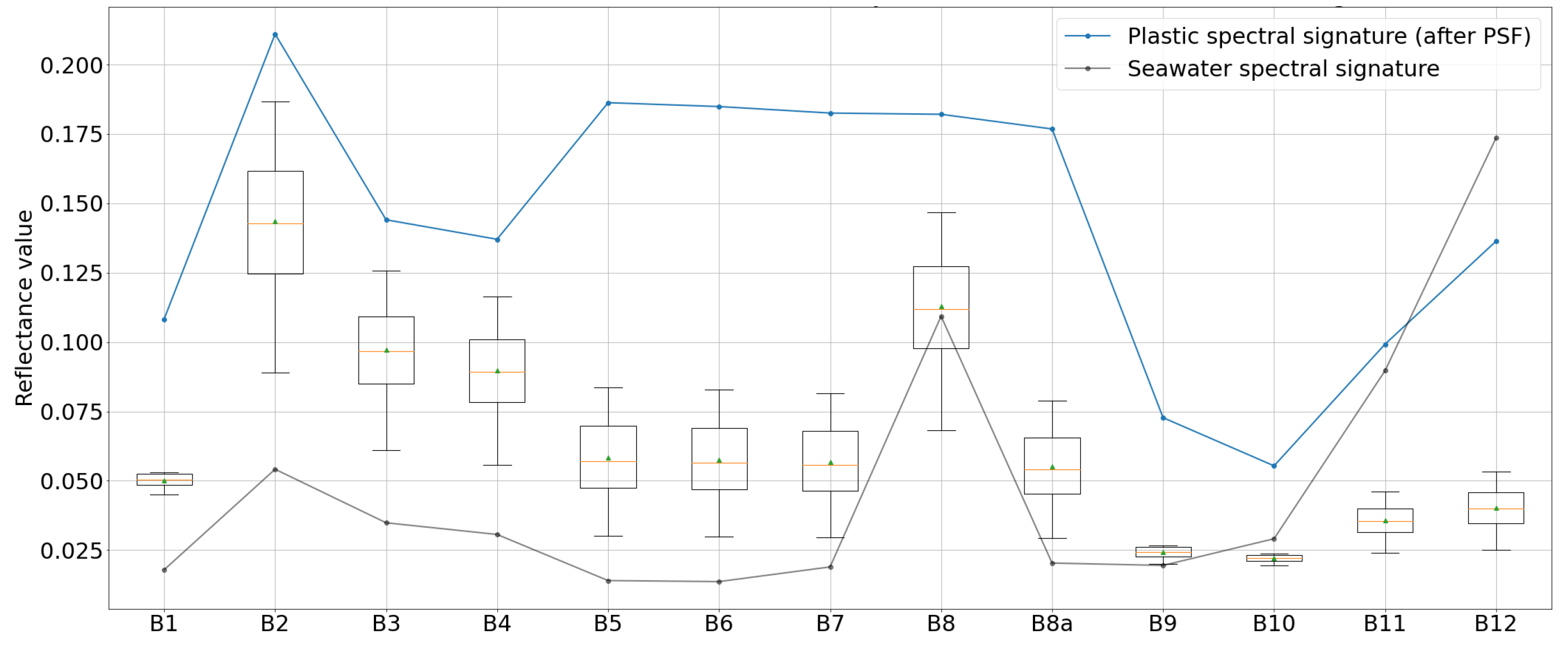
To assess the effect of aliasing over one scene, it is necessary to observe the results of the sampling with all the possible jitters and to see how the reflectance values are affected. For a band with a GSD of 10 m, all of the 100 jitters are used for the sampling; for a band with a GSD of 20 m, all of the 400 jitters are used and for a band with GSD of 60 m, all of the 3600 jitters are used. In order to collect the result of all of the jitters and to compare it, the scene described in Section 2.2.3. (patch size of 30   m × 30   m ) has been sampled as many times as needed by going through all the jitters and without applying noise as the focus is put on the sampling process. For each sampling, only the value of the pixel with the highest reflectance value was collected (recall that the seawater has a minimum reflectance). All these values have been displayed in boxplots, one boxplot for each band, and are presented in Figure 7. The blue line corresponds to the spectral signature of wet bottles frame [25] after the convolution with the PSFs; the closer the reflectance values are from this line, the more accurate the sampling of the satellite is. The dark line corresponds to the seawater spectral signature from [35]. For bands B02, B03, B04, and B08 (GSD = 10 m), the boxplots are centered around the same reflectance value and are close to the spectral signature of plastic (blue line). This means that for the particular size 30   m × 30   m , the data collected by S2 are not subject to aliasing artifacts. The boxplots of bands B01, B09, and B10 are more spread meaning that the sampling of the scene depends on the jitter and thus that these bands are sensitive to the aliasing effect. As for the bands with a GSD of 20 m, the boxplots are spread but the values meet with the spectral signature of plastic. All in all, based on the simulations, a plastic patch of size 30   m × 30   m can be accurately detected by S2 for the bands with a GSD of 10 m. The results of the other bands are less exploitable.
As a comparison, Figure 8 shows the same plots but with a plastic patch of size 10   m × 10   m . This time, the blue line does not meet any of the boxplots and the boxes for the bands of 10 m resolution have spread values. The boxplots of bands B01, B09 and B10 (GSD = 60 m) seem to be centered around the same value but this is because no plastic is detected at all. A 10   m × 10   m plastic patch made out of plastic bottles such as the one deployed by [10] is strongly affected by aliasing.
Though small plastic patches such as a 10   m × 10   m patch are observable from S2, the reflectance values are not reliable because of aliasing. By comparing the results from a 30   m × 30   m patch and from a 10   m × 10   m , we can observe that the aliasing effect is less significant for larger patches. We generated images with plastic patches made out of a common plastic material and of various sizes (from 1 m to 150 m). We assessed the threshold above which aliasing does not occur. For rectangular shapes, the minimum size required to overcome aliasing for bands with GSD = 10 m is approximately 25   m × 25   m whereas for the bands with GSD = 20 m, the required size is 40   m × 40   m . For circular shapes, the minimum size required to avoid aliasing is R = 15 m for the bands with GSD = 10 m and R = 25 m for bands with GSD = 20 m. All results are summarized in Table 2. We therefore recommend to have these orders of size in mind when using S2 data in order to avoid aliasing, but they are not strict limits. A plastic patch of size 23   m × 23   m will be under the size limit but the impact of aliasing might not be significant or at least, less important than for a 10   m × 10   m patch.

2.2.5. Description of the Generated Dataset

A set of simulated images has been generated to train several classifiers to discriminate between seawater and patches of debris. In total, 1110 images describing various scenes have been generated, with 15 different materials, be it plastic (e.g., bags or bottles) or not (e.g., wood). For each material, 74 images have been generated by changing the shape, the size, the rotation and the fraction of coverage. For instance, the smallest circular shape is 1 m radius and the biggest one is 75 m radius; the fraction of coverage goes from 40 % to 90 % . The lower bound was chosen by calculating the ratio between, on the one hand, the plastic response from one of the images of PLP, and on the other hand, a simulated plastic with 100 % coverage.
The final dataset is composed of the shuffled collection of the pixels of all the images. One pixel is represented by a vector made of the 13 reflectance values of the S2 spectral bands, and a Boolean that specifies if the pixel contains debris or not. Based on the material type, we created 3 classes. Class 0 is for seawater pixels, class 1 is for pixels containing plastic, and class 2 for pixels containing wood. In total, the dataset is composed of 166,619 pixels: 150,000 pixels of seawater, 13,291 pixels of plastic and 3328 pixels of wood. It is then a rather unbalanced dataset, similar to the S2 data.

2.2.6. Training of a Classifier on Synthetic Data

For the sake of simplicity, only a Random Forest classifier [40] was chosen to test automated plastic detection. When large datasets are available, a Random Forest is a good choice given its accuracy and intelligibility. This classifier is trained on individual pixels from the generated images. This ensures that all pixels from a patch can be classified, without regard for the shape or the size of the patch. This also allows the classifier to correctly classify patches that are made out of multiple materials. We split the dataset into training, validation and testing sets with ratios 0.8, 0.1, and 0.1, respectively. We used the Random Forest classifier from the scikit learn package version 0.24.2 [41]. Various parameters have been tested by generating new datasets. On the S2 case, the Random Forest with default parameters prove to have satisfying results.
On the synthetic data, the key performance metrics of the classifier are very high: superior or equal to 0.99 for the f1-score, precision, and recall. The classifier was able to successfully classify seawater, plastic, or wood pixels. These high results are mostly due to the fact that the simulated materials are easily separable. The classifier performs well on a pixel by pixel case, but it is also worth investigating its performances on an image by image case. By this, we mean performing the assessment of the same classifier on the entirety of an image, not training a separate one that takes a whole image as input. We expect it to be sensitive to the size of the patch due to aliasing: the smaller it is, the harder it will be to detect, thus inducing lower f1-score, precision, and recall. To test this, we generated a set of 45 scenes with patches of circular shape, with radius ranging between 1 m and 100 m. The material type for all images was set to wet bottles frame. To observe the impact on detection of the artifacts induced by the sampling process, we randomly picked 10 jitters for each image.
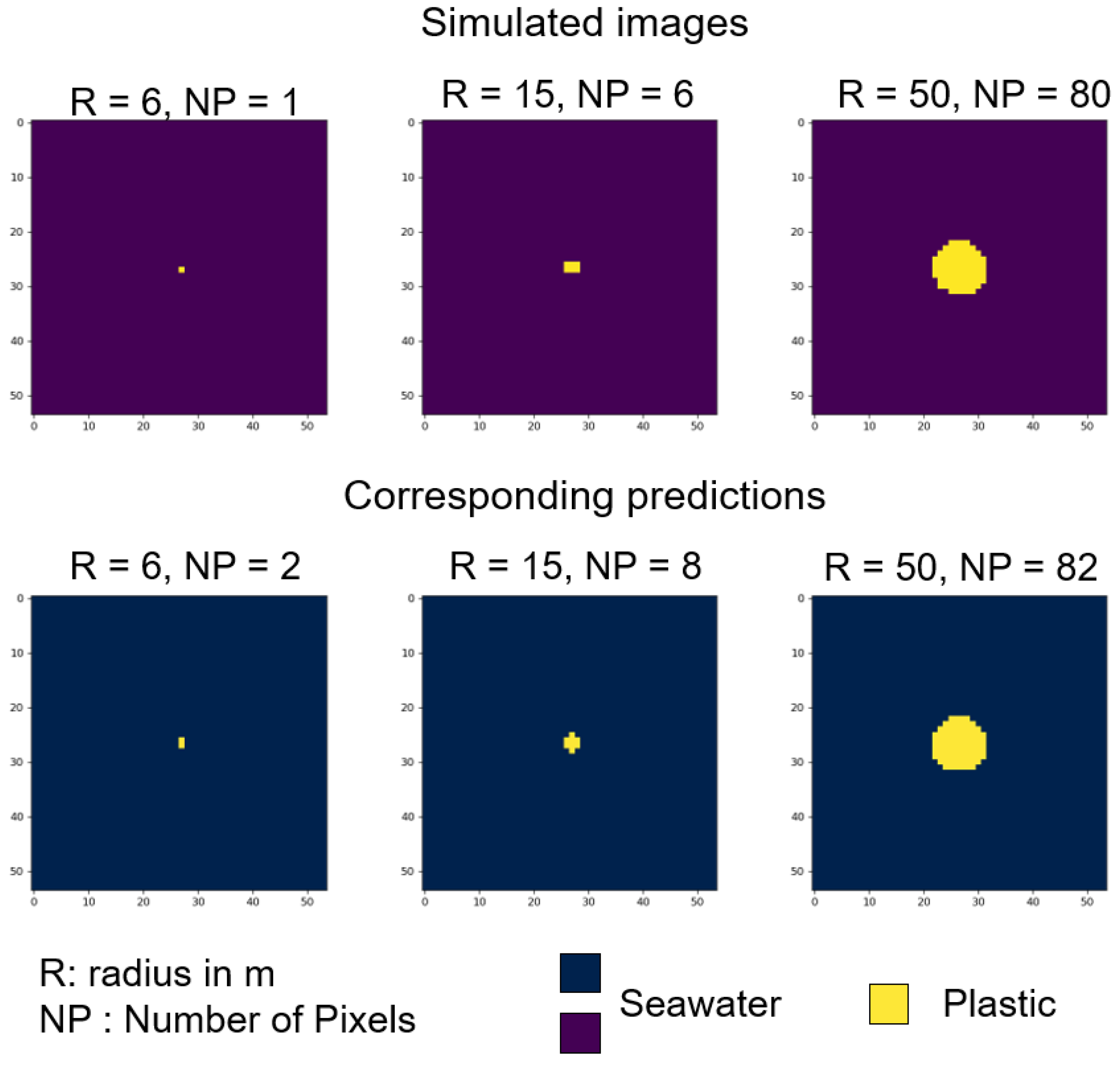
Figure 9 shows three particular cases of inaccurate prediction. At the top, the masks of simulated images are displayed and at the bottom, the results of the prediction by the Random Forest classifier. For all for three images, we chose a particular jitter to plot the images. The results do not drastically change between jitters. On these images, we can see the aliasing effect particularly well on the third one (R = 50 m). Some of the pixels at the border are expected to be plastic but because of the sampling and the jitter, the left bottom border have water values instead. In all images, we can see that some of the surrounding water pixels are mis-classified as plastic (one or two false positives for each image). However, at the scale of the patch, the predictions are satisfactory.
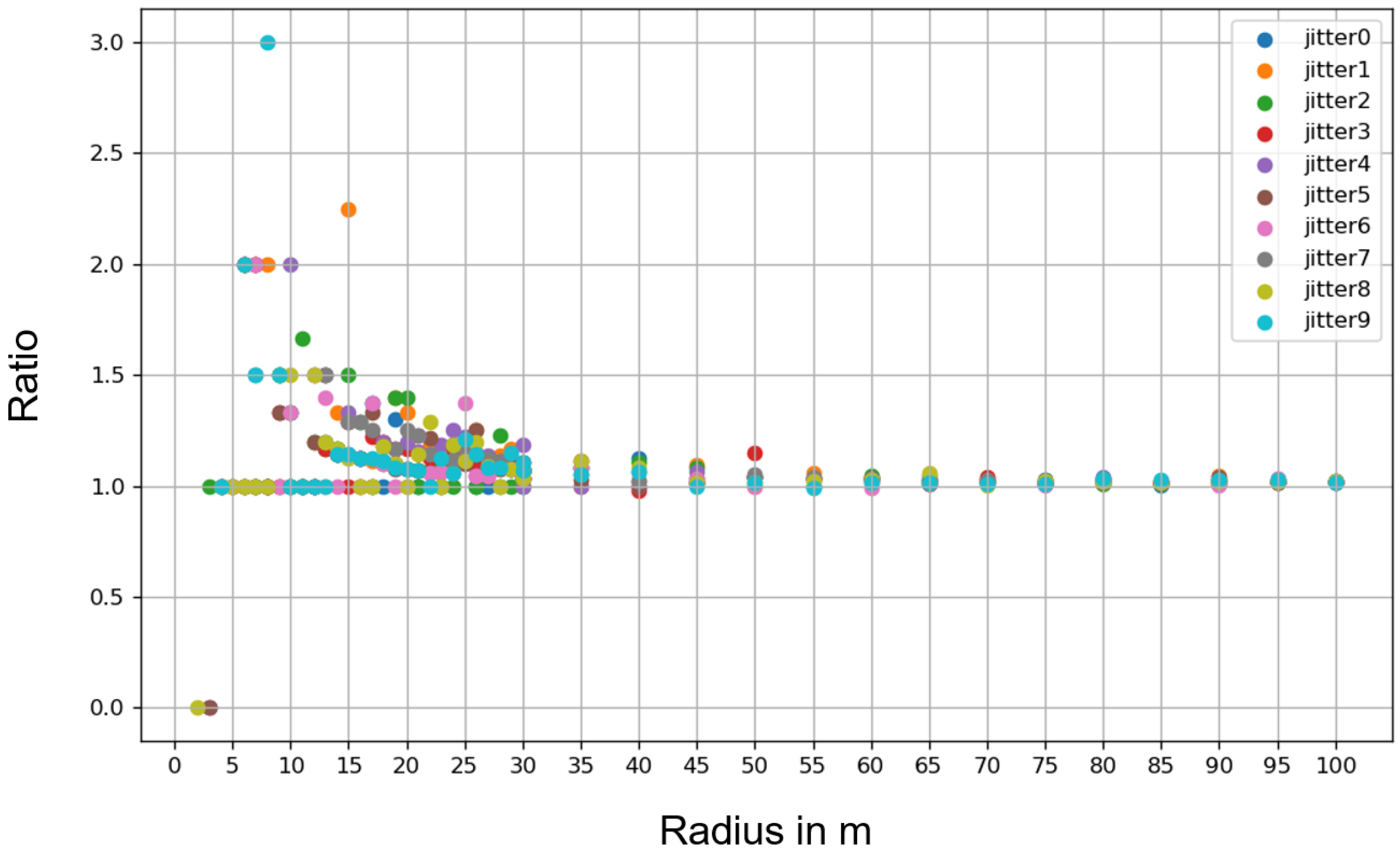
Afterwards, for each image and each jitter, we compared the number of plastic pixels on the simulated image and the number of plastic pixels predicted. Figure 10 shows the ratio of the predicted number by the simulated number depending on the radius of the patch and per jitter.
We can see that for small radii (under 15 m), the ratio can reach 2, meaning that there were 2 times more plastic predicted that there actually was. Between 15 m and 30 m, the ratio stabilizes to 1: for bigger patches, the classifier is able to predict the correct number of plastic pixels. When the ratio is 0, it means that the classifier did not detect any plastic but some were labeled as such. When the classifier predicts the wrong amount of plastic, the error is not aberrant. For the 8 m radius, the classifiers predicts 3 times more plastic than labeled: it actually predicts 3 pixels of plastic when only one is simulated.

3. Results on Real Images

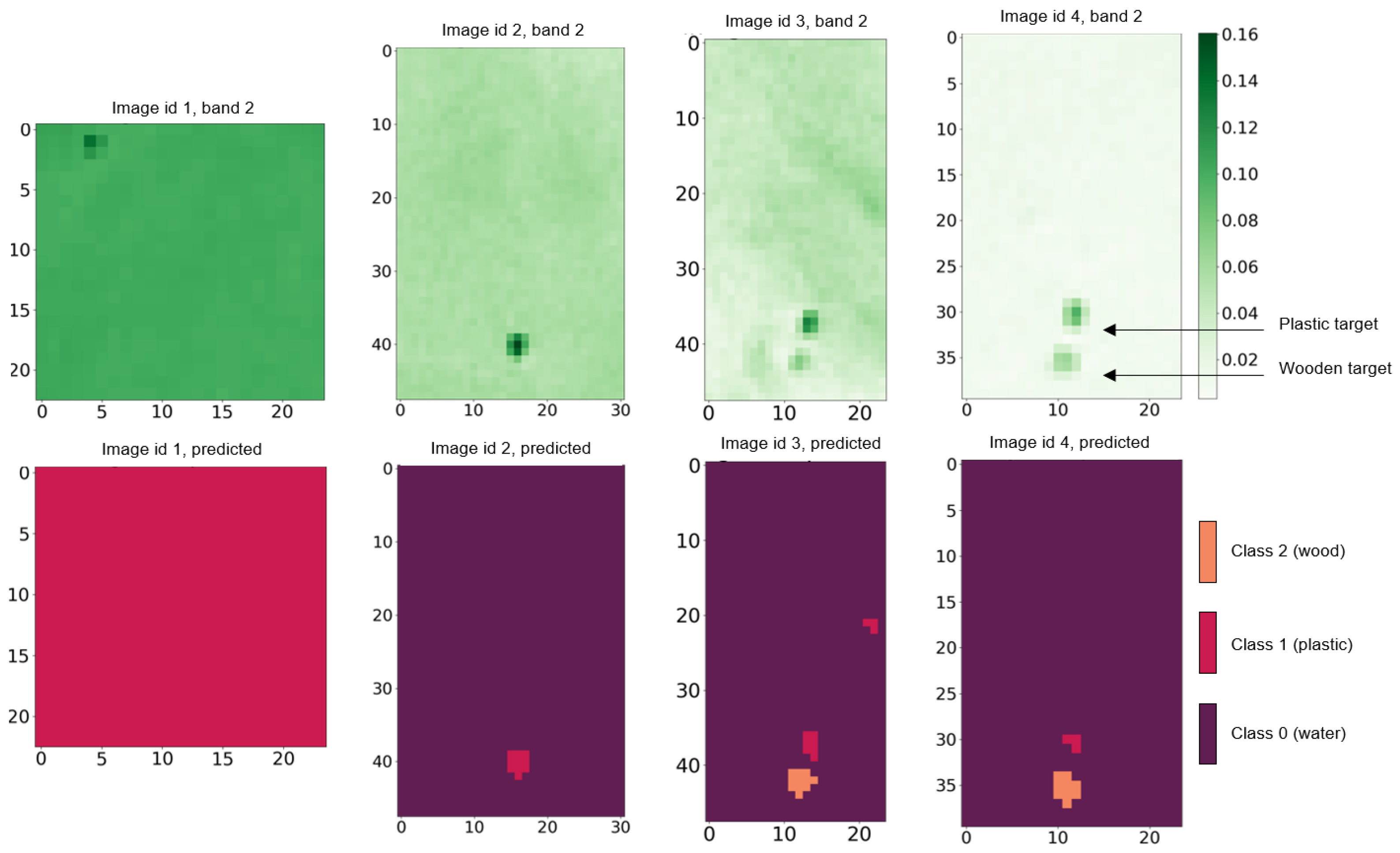
We tested the classifier developed in Section 2.2.6 on real images, i.e., S2 images containing plastic and wood patches. We collected four images from the different PLP experiments. One contains a plastic target of 10   m × 10   m , one contains a plastic target of 28 m diameter and the last two contain two 28 m diameter targets, one of plastic and one of wood. All of the images are described in Table 3. We collected only level 2A images, i.e., atmospheric corrected images, in accordance with our model (see Hypothesis H3 in Section 2). These images were chosen due to the large size of some of the targets (which should ensure that the aliasing artifacts are not too severe), the presence of multiple materials and the different conditions in which they were taken (for example, in image 4 of Figure 11, the targets are biofouled).
Figure 11 presents the results obtained. The images collected from S2 are displayed on the first row for B02 and on the second row are the predicted heatmaps (see legend). The True Positive (TP) and False Positive (FP) values for plastic and wood pixels are presented in Table 4 and Table 5.
On images 2, 3, and 4, the classifier correctly detected seawater, plastic, and wood patches. However, on image 1, it only predicted plastic. In order to better understand the cause of this mis-classification, we tested the classifier on another image from the PLP21 from the 11 June with the same scene as the one in image 2. For this image, the results obtained were the same as the ones obtained for image 1, i.e., most of the seawater pixels were classified as plastic. The common point to these 2 images are the seawater reflectance values: they were significantly higher than the seawater reflectance values we modeled and generated. Figure 12 shows the boxplots of the simulated plastic values and real seawater values. For both figures, the transparent boxplots contain simulated plastic values taken from our dataset and the averaged spectral signature of simulated water in dark blue. For both figures, the blue boxplots contain real seawater values. On the top, the real seawater values are collected from image 1 and from the image of the 11 June (600 seawater pixels). On the bottom, the real seawater values are collected from image 2, 3, and 4 (1200 pixels). We can see that, for image 1 and for the image of the 11 June (on the top of Figure 12), the real seawater values are higher than regular seawater values and overlap with the simulated plastic values. In this case, the spectral signature of simulated water does not meet the real seawater values for most bands. For this range of values, the classifier learns that the pixels are plastic pixels, thus explaining why it classifies real seawater pixels as plastic in image 1 (and the image from the 11 June not displayed here). In comparison, we can see that, for image 2, 3, and 4 (on the bottom of Figure 12), the real seawater values are lower and meet with the spectral signature of simulated water. This shows the sensitivity of the prediction to extreme values of seawater reflectance values.

4. Discussion

The satellite model was developed based on hypotheses, that we discuss now. For instance, to simplify, we neglected the effects of the atmosphere on the reflectance (H3 in Section 2.1.2). The images obtained by our simulation are thus comparable to level 2A S2 products i.e., atmospheric corrected images, assuming this correction is perfect. These level 2A images are obtained after processing level 1C images by a default atmospheric correction processor called Sen2cor, which was developed by ESA. However, some studies question the Sen2Cor algorithm: [10] showed that Sen2Cor produces higher reflectance values for water constituents, which could interfere with floating plastics detection. An alternative that has been used in some studies is the ACOLITE algorithm [20]. It would be interesting to add the effects of atmosphere on the reflectance in order to generate images closer to S2 level 1C products.
When testing the classifier on real images, we noticed that our model of seawater should be improved, as this seems to be a major driver of a robust performance. For now, we load the spectral signature of seawater from the USGS library [35] but this not diverse enough. Particularly, they provide with spectral signatures for deep ocean and coastal waters, but the values are exactly the same. Collecting more spectral data on seawater under various conditions (different wave types and amplitudes, different viewing and lighting angles, etc.) will enable the development of more realistic seawater models.
Another phenomenon that could lead to distorted reflectance values is sun glint–strong specular highlights on water. In particular cases, the radiances measured by the satellite from seawater could be significantly higher, leading to mis-predictions. Modeling sun glint could increase the robustness of classifiers in operating conditions. Another option would be to attempt to rectify the real images before predicting on them by using techniques such as those presented in [42].
Currently, as stated in Hypothesis H5, we do not take into account the positions of the Earth and Sun, while a more realistic model would be harder to define, taking spatial parameters into account would allow the generation of more varied datasets. Accurate modeling of the Sun–Earth–Satellite system could also simplify the task of modeling sun glint.
Although our implementation of the framework is currently configured to generate images that attempt to mimic those produced by S2, this can be easily adapted. Products from other satellites can be simulated by changing the definitions of the bands: wavelength, sensitivity, PSF, and resolution. New materials can be easily added and existing materials can be modified by changing values in the material database. It would also be easy to generalize the shape parametrization to any polygon. The noise model can be adapted by changing the σ value or even the distribution. Adjustment of the noise could force classifiers to be less dependent on the conditions imposed by our hypotheses and thus be more likely to generalize well. We conceived the simulator specifically so that it could be used in other situations. See Section 2.2.1 for instructions on how to access the code.
Currently, our debris patches are only composed of one material. Moreover, the S2 images that we tested on are of artificial plastic targets. However, as previously stated, the real life patches tend to be formed of multiple materials. A model of mixed-material patches could therefore enhance the performances of classifiers in real situations. This is why experiments with real targets of different types and of different ages should be seen as complementary to the simulation based approach in this paper. These experiments should be used both to enrich the simulation tool and to test the resulting machine learning algorithms.
Finally, when trained on simulated data, classifiers, such as the Random Forest we tested, can prove viable for marine litter detection. Currently, we trained the Random Forest on a dataset pixel by pixel and used it to predict the presence of plastic or other material, but it could also be trained to classify the exact material present in a pixel. Moreover, other classifiers could be trained to predict on an image by image basis. A particularly interesting one could be a Convolutional Neural Network (CNN) [43]. Adding new features such as bands combination with indexes such as those in [8] is another option for investigating automated marine debris detection. Such classifiers, with a great number of parameters, typically require large datasets to be trained and this is where our framework, with refined parameters, could bring the most added value.
In the future, we believe that a mixed approach, one that combines new data collection campaigns and machine learning algorithms trained on synthetic data will lead to a dramatic improvement in the current state of the art of remote sensing marine debris detection. The main advantages of using a physical approach for the generation of synthetic data is that, compared to the other approaches presented in the introduction, it is easy to reproduce with openly available resources. Furthermore, the bias introduced by our simplifications can be controlled by adapting the physics of the model, as previously discussed.
We have faith in a symbiotic relationship, where new in situ data is used to validate the various detection algorithms and where synthetic data is used to inform and guide future data collection and cleanup campaigns.

5. Conclusions

In this study, we tackled the issues of data scarcity and quality for marine litter monitoring from satellite by proposing a methodology based on the use of synthetic data. The goal is to reduce the risk of overfitting, a general goal in machine learning, which is almost impossible to avoid with the currently available data. We showed that machine learning algorithms that are trained on synthetic data transfer well to real-life conditions, thus helping to overcome the issue of data scarcity. We hope that our work will help further develop the uses of synthetic data for remote sensing applications.
Regarding the issue of data quality, we pointed out potential aliasing effects on S2 images of targets and noted their effects on the prediction. The aliasing effect has a huge influence on images containing plastic patches whose size is lower than or close to the GSD, but is less important (or non-existent) for plastic patches of larger sizes. To be sure to collect reliable data using S2, we found that the plastic patches should not be smaller than 25   m × 25   m for rectangle shapes and of 15 m radius for circular shapes. This result applies only for spectral bands with GSD = 10 m; for spectral bands with lower spatial resolution the size limit increases. These size limits are not strict and should be seen as recommendations.
Finally, even though we illustrated a proof of concept implementation of our methodology on the task of macro-plastic detection from S2 data, the simulator we developed is easily extendable to other satellites and other types of marine pollution. The models presented are adaptable and versatile. We strongly believe that following the guidelines established by our methodology will enable the development of novel algorithms for marine pollution detection from satellite data. The methodology could be used not only to train classifiers but also to foresee which existing (or future) satellites are more suited for plastic detection and to answer questions such as: Are there any other interesting wavelengths for plastic detection? How does the response change based on the plastic type and what plastic types are more easily detectable?

Author Contributions

Conceptualization, M.N., S.T. and P.B.; methodology, S.T. and P.B.; software, M.N., L.I. and M.S.; formal analysis, M.S.; investigation, M.N.; data curation, M.N., L.I. and M.S.; writing—original draft preparation, M.N.; writing—review and editing, L.I., S.T. and P.B.; visualization, M.N., L.I. and M.S.; supervision, S.T. and P.B. All authors have read and agreed to the published version of the manuscript.

Funding

This research received no external funding.

Data Availability Statement

See Section 2.2.1 for instructions on how to access the data that was used in this study and the full source code of the simulator.

Conflicts of Interest

The authors declare no conflict of interest.

References

  1. Aoyama, T. Extraction of marine debris in the Sea of Japan using high-spatial-resolution satellite images. In Remote Sensing of the Oceans and Inland Waters: Techniques, Applications, and Challenges; Frouin, R.J., Shenoi, S.C., Rao, K.H., Eds.; SPIE International Society for Optics and Photonics: Bellingham, WA, USA, 2016; Volume 9878, pp. 213–219. [Google Scholar] [CrossRef]
  2. Novelli, A.; Tarantino, E. The contribution of Landsat 8 TIRS sensor data to the identification of plastic covered vineyards. In Proceedings of the Third International Conference on Remote Sensing and Geoinformation of the Environment (RSCy2015), Paphos, Cyprus, 16–19 March 2015; Hadjimitsis, D.G., Themistocleous, K., Michaelides, S., Papadavid, G., Eds.; SPIE International Society for Optics and Photonics: Bellingham, WA, USA, 2015; Volume 9535, pp. 441–449. [Google Scholar] [CrossRef]
  3. Garaba, S.P.; Aitken, J.; Slat, B.; Dierssen, H.M.; Lebreton, L.; Zielinski, O.; Reisser, J. Sensing Ocean Plastics with an Airborne Hyperspectral Shortwave Infrared Imager. Environ. Sci. Technol. 2018, 52, 11699–11707. [Google Scholar] [CrossRef] [PubMed]
  4. Garaba, S.P.; Dierssen, H.M. An airborne remote sensing case study of synthetic hydrocarbon detection using short wave infrared absorption features identified from marine-harvested macro- and microplastics. Remote Sens. Environ. 2018, 205, 224–235. [Google Scholar] [CrossRef]
  5. Maximenko, N.; Corradi, P.; Law, K.L.; Van Sebille, E.; Garaba, S.P.; Lampitt, R.S.; Galgani, F.; Martinez-Vicente, V.; Goddijn-Murphy, L.; Veiga, J.M.; et al. Toward the Integrated Marine Debris Observing System. Front. Mar. Sci. 2019, 6, 447. [Google Scholar] [CrossRef] [Green Version]
  6. Martínez-Vicente, V.; Clark, J.R.; Corradi, P.; Aliani, S.; Arias, M.; Bochow, M.; Bonnery, G.; Cole, M.; Cózar, A.; Donnelly, R.; et al. Measuring Marine Plastic Debris from Space: Initial Assessment of Observation Requirements. Remote Sens. 2019, 11, 2443. [Google Scholar] [CrossRef] [Green Version]
  7. ESA. Sentinel-2 ESA’s Optical High Resolution Mission for GMES Operational Services; European Space Agency: Paris, France, 2012. [Google Scholar]
  8. Biermann, L.; Clewley, D.; Martinez-Vicente, V.; Topouzelis, K. Finding Plastic Patches in Coastal Waters using Optical Satellite Data. Sci. Rep. 2020, 10, 5364. [Google Scholar] [CrossRef] [Green Version]
  9. Kikaki, K.; Kakogeorgiou, I.; Mikeli, P.; Raitsos, D.E.; Karantzalos, K. MARIDA: A benchmark for Marine Debris detection from Sentinel-2 remote sensing data. PLoS ONE 2022, 17, e0262247. [Google Scholar] [CrossRef]
  10. Topouzelis, K.; Papakonstantinou, A.; Garaba, S.P. Detection of floating plastics from satellite and unmanned aerial systems (Plastic Litter Project 2018). Int. J. Appl. Earth Obs. Geoinf. 2019, 79, 175–183. [Google Scholar] [CrossRef]
  11. Themistocleous, K.; Papoutsa, C.; Michaelides, S.; Hadjimitsis, D. Investigating Detection of Floating Plastic Litter from Space Using Sentinel-2 Imagery. Remote Sens. 2020, 12, 2648. [Google Scholar] [CrossRef]
  12. Topouzelis, K.; Papageorgiou, D.; Karagaitanakis, A.; Papakonstantinou, A.; Arias Ballesteros, M. Remote Sensing of Sea Surface Artificial Floating Plastic Targets with Sentinel-2 and Unmanned Aerial Systems (Plastic Litter Project 2019). Remote Sens. 2020, 12, 2013. [Google Scholar] [CrossRef]
  13. Goddijn-Murphy, L.; Williamson, B.J.; McIlvenny, J.; Corradi, P. Using a UAV thermal infrared camera for monitoring floating marine plastic litter. Remote Sens. 2022, 14, 3179. [Google Scholar] [CrossRef]
  14. Bao, Z.; Sha, J.; Li, X.; Hanchiso, T.; Shifaw, E. Monitoring of beach litter by automatic interpretation of unmanned aerial vehicle images using the segmentation threshold method. Mar. Pollut. Bull. 2018, 137, 388–398. [Google Scholar] [CrossRef]
  15. Martin, C.; Parkes, S.; Zhang, Q.; Zhang, X.; McCabe, M.F.; Duarte, C.M. Use of unmanned aerial vehicles for efficient beach litter monitoring. Mar. Pollut. Bull. 2018, 131, 662–673. [Google Scholar] [CrossRef] [Green Version]
  16. Jakovljevic, G.; Govedarica, M.; Alvarez-Taboada, F. A deep learning model for automatic plastic mapping using unmanned aerial vehicle (UAV) data. Remote Sens. 2020, 12, 1515. [Google Scholar] [CrossRef]
  17. Geraeds, M.; van Emmerik, T.; de Vries, R.; bin Ab Razak, M.S. Riverine plastic litter monitoring using unmanned aerial vehicles (UAVs). Remote Sens. 2019, 11, 2045. [Google Scholar] [CrossRef] [Green Version]
  18. Andriolo, U.; Gonçalves, G.; Sobral, P.; Bessa, F. Spatial and size distribution of macro-litter on coastal dunes from drone images: A case study on the Atlantic coast. Mar. Pollut. Bull. 2021, 169, 112490. [Google Scholar] [CrossRef]
  19. Yang, Z.; Yu, X.; Dedman, S.; Rosso, M.; Zhu, J.; Yang, J.; Xia, Y.; Tian, Y.; Zhang, G.; Wang, J. UAV remote sensing applications in marine monitoring: Knowledge visualization and review. Sci. Total. Environ. 2022, 838, 155939. [Google Scholar] [CrossRef]
  20. Basu, B.; Sannigrahi, S.; Sarkar Basu, A.; Pilla, F. Development of Novel Classification Algorithms for Detection of Floating Plastic Debris in Coastal Waterbodies Using Multispectral Sentinel-2 Remote Sensing Imagery. Remote Sens. 2021, 13, 1598. [Google Scholar] [CrossRef]
  21. Sannigrahi, S.; Basu, B.; Basu, A.S.; Pilla, F. Development of automated marine floating plastic detection system using Sentinel-2 imagery and machine learning models. Mar. Pollut. Bull. 2022, 178, 113527. [Google Scholar] [CrossRef]
  22. Taggio, N.; Aiello, A.; Ceriola, G.; Kremezi, M.; Kristollari, V.; Kolokoussis, P.; Karathanassi, V.; Barbone, E. A Combination of Machine Learning Algorithms for Marine Plastic Litter Detection Exploiting Hyperspectral PRISMA Data. Remote Sens. 2022, 14, 3606. [Google Scholar] [CrossRef]
  23. Anthony, M.; Bartlett, P.L.; Bartlett, P.L. Neural Network Learning: Theoretical Foundations; Cambridge University Press: Cambridge, UK, 1999; Volume 9. [Google Scholar]
  24. Cao, Y.; Huang, X. A coarse-to-fine weakly supervised learning method for green plastic cover segmentation using high-resolution remote sensing images. ISPRS J. Photogramm. Remote Sens. 2022, 188, 157–176. [Google Scholar] [CrossRef]
  25. Knaeps, E.; Strackx, G.; Meire, D.; Sterckx, S.; Mijnendonckx, J.; Moshtaghi, M. Hyperspectral reflectance of marine plastics in the VIS to SWIR. Sci. Rep. 2020. [Google Scholar] [CrossRef]
  26. Yu, X.; Wu, X.; Luo, C.; Ren, P. Deep learning in remote sensing scene classification: A data augmentation enhanced convolutional neural network framework. GIScience Remote Sens. 2017, 54, 741–758. [Google Scholar] [CrossRef] [Green Version]
  27. Yan, Y.; Tan, Z.; Su, N. A Data Augmentation Strategy Based on Simulated Samples for Ship Detection in RGB Remote Sensing Images. ISPRS Int. J. Geo-Inf. 2019, 8, 276. [Google Scholar] [CrossRef] [Green Version]
  28. Tournadre, B.; Gschwind, B.; Thomas, C.; Saboret, L.; Blanc, P. Simulating Clear-Sky Reflectance of the Earth as Seen by Spaceborne Optical Imaging Systems with a Radiative Transfer Model; EGU General Assembly: Munich, Germany, 2019; Volume 21, p. 18647. [Google Scholar] [CrossRef]
  29. Hoeser, T.; Kuenzer, C. SyntEO: Synthetic dataset generation for earth observation and deep learning—Demonstrated for offshore wind farm detection. ISPRS J. Photogramm. Remote Sens. 2022, 189, 163–184. [Google Scholar] [CrossRef]
  30. Kong, F.; Huang, B.; Bradbury, K.; Malof, J. The Synthinel-1 dataset: A collection of high resolution synthetic overhead imagery for building segmentation. In Proceedings of the IEEE/CVF Winter Conference on Applications of Computer Vision, Snowmass Village, CO, USA, 1–5 March 2020; pp. 1814–1823. [Google Scholar]
  31. Fourest, B.; Lier, V. (Eds.) Satellite Imagery from Acquisition Principles to Processing of Optical Images for Observing the Earth; Cépaduès Editions: Toulouse, France, 2012. [Google Scholar]
  32. Blanc, P.; Wald, L. A review of earth-viewing methods for in-flight assessment of modulation transfer function and noise of optical spaceborne sensors. HAL Open Sci. 2009, 1–38. [Google Scholar]
  33. Shannon, C.E. A Mathematical Theory of Communication. Bell Syst. Tech. J. 1948, 27, 379–423. [Google Scholar] [CrossRef] [Green Version]
  34. Moshtaghi, M.; Knaeps, E.; Sterckx, S.; Garaba, S.; Meire, D. Spectral reflectance of marine macroplastics in the VNIR and SWIR measured in a controlled environment. Sci. Rep. 2021, 11, 5436. [Google Scholar] [CrossRef]
  35. Kokaly, R.F.; Clark, R.N.; Swayze, G.A.; Livo, K.E.; Hoefen, T.M.; Pearson, N.C.; Wise, R.A.; Benzel, W.M.; Lowers, H.A.; Driscoll, R.L.; et al. USGS Spectral Library Version 7; Technical Report; USGS: Reston, VA, USA, 2017. [Google Scholar] [CrossRef]
  36. USGS Spectral Library. Spectral Library Version 7. 2017. Available online: https://crustal.usgs.gov/speclab/SNTL2.php?quick_filter= (accessed on 13 November 2021).
  37. ESA. Sentinel-2 Spectral Response Functions (S2-SRF). 2017. Available online: https://sentinels.copernicus.eu/web/sentinel/user-guides/sentinel-2-msi/document-library/-/asset_publisher/Wk0TKajiISaR/content/sentinel-2a-spectral-responses (accessed on 12 October 2021).
  38. Source Code of the Simulator. Available online: https://code.sophia.mines-paristech.fr/Luca/ademal (accessed on 5 August 2021).
  39. Topouzelis, K.; Papageorgiou, D. Plastic Litter Project 2021. Available online: http://plp.aegean.gr/category/experiment-log-2021/ (accessed on 11 October 2021).
  40. Breiman, L. Random forests. Mach. Learn. 2001, 45, 5–32. [Google Scholar] [CrossRef] [Green Version]
  41. Pedregosa, F.; Varoquaux, G.; Gramfort, A.; Michel, V.; Thirion, B.; Grisel, O.; Blondel, M.; Prettenhofer, P.; Weiss, R.; Dubourg, V.; et al. Scikit-learn: Machine Learning in Python. J. Mach. Learn. Res. 2011, 12, 2825–2830. [Google Scholar]
  42. Kay, S.; Hedley, J.; Lavender, S. Sun Glint Correction of High and Low Spatial Resolution Images of Aquatic Scenes: A Review of Methods for Visible and Near-Infrared Wavelengths. Remote Sens. 2009, 1, 697. [Google Scholar] [CrossRef] [Green Version]
  43. LeCun, Y.; Boser, B.; Denker, J.S.; Henderson, D.; Howard, R.E.; Hubbard, W.; Jackel, L.D. Backpropagation Applied to Handwritten Zip Code Recognition. Neural Comput. 1989, 1, 541–551. [Google Scholar] [CrossRef]
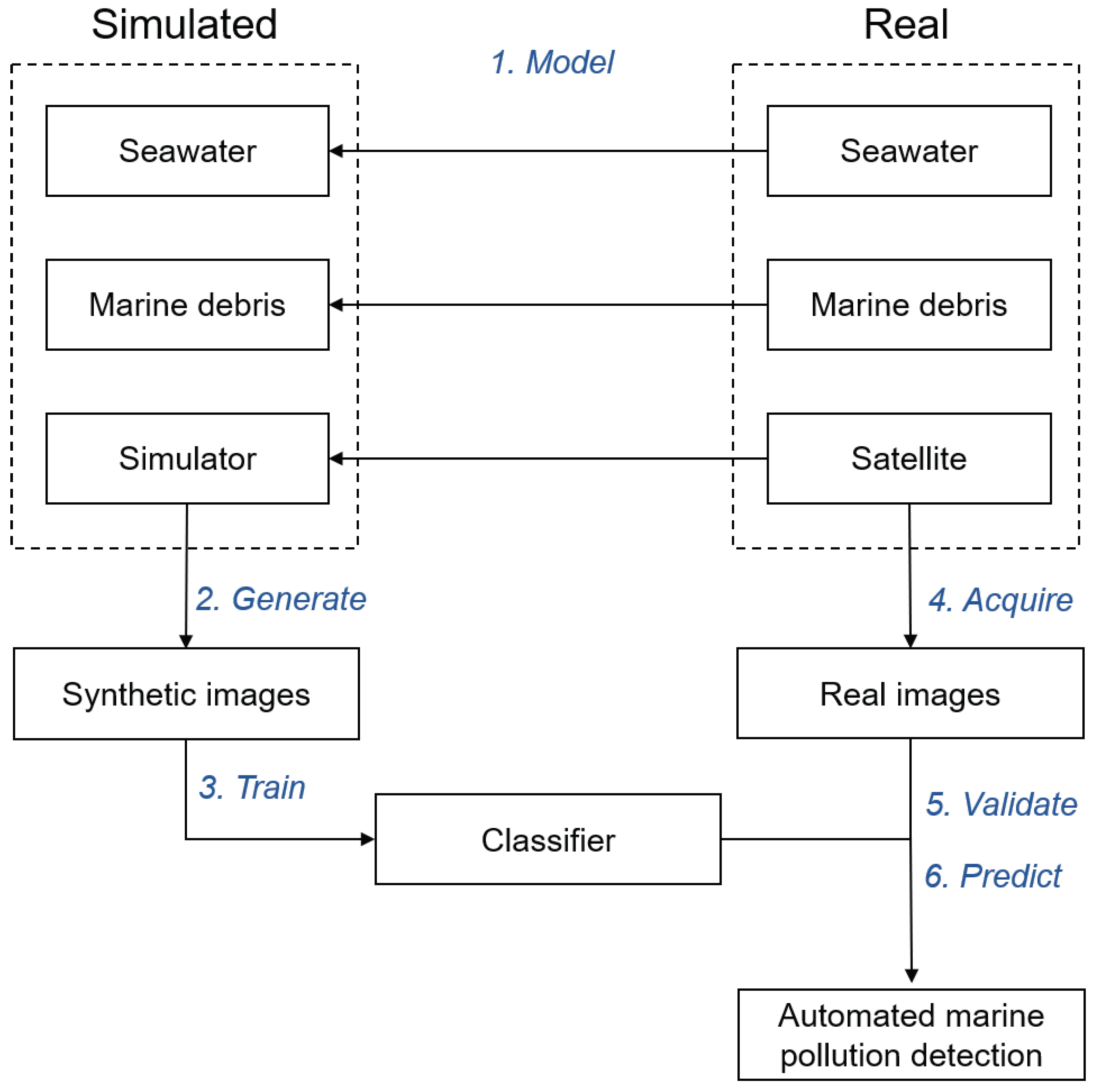
Figure 1. Definition of the methodology.
Remotesensing 14 06102 g001
Figure 2. Simplified illustration of the interaction between the main quantities taken into account in the model.
Remotesensing 14 06102 g002
Figure 3. Illustration of aliasing effects due to differences in sampling. (a) Image after convolution with the PSF. Jitter 5 , 5 is represented by the red dots. (b) Image after sampling with jitter 5 , 5 . (c) Image after convolution with the PSF. Jitter 1 , 1 is represented by the red dots. (d) Image after sampling with jitter 1 , 1 .
Remotesensing 14 06102 g003
Figure 4. Illustration of the inputs and outputs of the simulation.
Remotesensing 14 06102 g004
Figure 5. Simulated images of a 30   m × 30   m plastic patch made out of wet bottles frame for B01 and B02 only; with and without noise.
Remotesensing 14 06102 g005
Figure 6. In orange, the spectral signature extracted from a 28 m diameter target deployed for the PLP21. Image filename: S2A_MSIL2A_20210611T085601_N0300_R007_T35SMD_20210611T121904. In blue, the spectral signature of simulated plastic with the inputs mentioned in Section 2.2.3. The fraction of plastic was set to 0.6 to match the fraction of plastic of the HDPE mesh.
Remotesensing 14 06102 g006
Figure 7. Results of all the possible jitters for each band by selecting the maximum reflectance values. Plastic patch of size 30   m × 30   m . The triangle represents the average of the corresponding dataset and the orange line, the median.
Remotesensing 14 06102 g007
Figure 8. Results of all the possible jitters for each band by selecting the maximum reflectance values. Plastic patch of size 10   m × 10   m . The triangle represents the average of the corresponding dataset and the orange line, the median.
Remotesensing 14 06102 g008
Figure 9. Comparison between the masks of simulated images (top) and the corresponding predictions for each image (bottom) for inaccurate prediction.
Remotesensing 14 06102 g009
Figure 10. Ratio of the number of plastic pixels detected on the number of plastic pixels simulated depending on the radius of the patch and for 10 different jitters.
Remotesensing 14 06102 g010
Figure 11. The predictions of the classifier on S2 real images. S2 images presented in Table 3 are displayed on the first row for band B02. Second row present the predictions obtained by the classifier. When there are two patches on the image, the top one is plastic and the bottom one is wood. (For interpretation of the references to color in this figure legend, the reader is referred to the web version of this article.)
Remotesensing 14 06102 g011
Figure 12. Boxplots of the simulated plastic values and real seawater values. For both figures, the transparent boxplots contain simulated plastic values taken from our dataset and the averaged spectral signature of simulated water, the dark blue line. For both figures, the blue boxplots contain real seawater values. On the top, the real seawater values are collected from image 1 and from the image of the 11 June (600 seawater pixels). On the bottom, the real seawater values are collected from image 2, 3, and 4 (1200 pixels).
Remotesensing 14 06102 g012
Table 1. Table of the cut-off frequencies and Nyquist frequencies for each band of Sentinel-2.
BandCentral Wavelength
(nm)
Spatial Resolution
(GSD in m)
Nyquist Frequency
fn(m 1 )
Cut-Off Frequency
fc(m 1 )
Ratio
f c f n
B01443600.0080.4353.75
B02490100.050.397.8
B03560100.050.346.8
B04665100.050.295.8
B05705200.0250.2710.8
B06740200.0250.2510
B07783200.0250.249.6
B08842100.050.234.6
B08a865200.0250.228.8
B09945600.0080.2025
B101380600.0080.1417.5
B111610200.0250.124.8
B122190200.0250.083.2
Table 2. Table of the minimum sizes recommended to ensure S2 data reliability, i.e., to avoid aliasing.
ShapeRectangleCircle
GSD
GSD = 10 m
(B2, B3, B4, B8)
25   m × 25   m R = 15 m
GSD = 20 m
(B5, B6, B7, B8a, B11, B12)
40   m × 40   m R = 25 m
GSD = 60 m
(B1, B9, B10)
120   m × 120   m R = 70 m
Table 3. Table describing the images collected from S2 containing plastic patches.
IDLocationImage FilenameDate of AcquisitionDescription
1Mytilene, GreeceS2A_MSIL2A_20180607T085601_N0208_R007_T35SMD_20180607T1149197 July 2018 10   m × 10   m target
of plastic bottles
2Gulf of Gera, GreeceS2A_MSIL2A_20210611T085601_N0300_R007_T35SMD_20210611T12190411 June 202128 m diameter target
HDPE mesh
3Gulf of Gera, GreeceS2A_MSIL2A_20210701T085601_N0301_R007_T35SMD_20210701T1250291 July 2021two 28 m diameter targets
HDPE mesh and wood
4Gulf of Gera, GreeceS2A_MSIL2A_20210721T085601_N0301_R007_T35SMD_20210721T12103521 July 2021two 28 m diameter targets
HDPE mesh and wood biofouled
Table 4. Table with the true and false positive numbers for each S2 image.
Image IDNumber of Plastic PixelsTPFP
140552
210100
31073
4730
Table 5. Table with the true and false positive numbers for S2 images 2 and 3.
Image IDNumber of Wood PixelsTPFP
312110
41490
Publisher’s Note: MDPI stays neutral with regard to jurisdictional claims in published maps and institutional affiliations.