Abstract
In recent years, radar emitter signal identification has been greatly developed via the utilization of deep learning and has achieved significant improvements in identification accuracy. However, with the continuous emergence of complex regime radars and the increasing complexity of the electromagnetic environment, some new kinds of radar emitter signals collected are not in sufficient quantities to satisfy the demand of deep learning. As a result, in this paper, we adopted the prototypical network (PN) belonging to metric-based meta-learning to realize few-shot radar emitter signal recognition with the aim of meeting the needs of modern electronic warfare. Additionally, considering the problems that may arise in the field of few-shot radar emitter signal recognition, such as discriminative location bias caused by a small number of base classes or the large difference between base classes and novel classes, we proposed an attention-balanced strategy to improve meta-learning. Specifically, each channel in the feature map is forced to make the same contribution in the distinguishment of different classes. In addition, for PN, taking into account that the feature vectors of each support sample in the class are different, we set a network to exploit the relation between each support sample in the same classes, and weighted each feature vector of the support samples according to the relation. Large quantities of experiments indicate that our algorithm possesses more advantages than other algorithms.
1. Introduction
Radar emitter signal recognition plays an important role in electronic intelligence systems and electronic support measure systems. It is mainly achieved with deep learning at present and achieves great performance. For instance, L. Yang proposed an improved multi-channel one-dimensional (1D) convolutional neural network (CNN) in [1] which effectively solved the problems of fusion feature extraction, unbalance, and insufficient fusion, realizing a higher recognition rate of radar emitter signals. In [2], Y. Pu utilized the two-dimensional time–frequency diagram of the main ridge polar coordinate domain of the ambiguity function as the input of a convolution neural network to realize the recognition of different radar signals and achieved a good recognition effect under a low signal–noise ratio (SNR). A method based on a deep residual shrinkage network (DRSN) is proposed by Zhang in [3], which greatly improved the ability to learn features from noisy signals. Within the increasingly complex electromagnetic environment, it appears that high-quality signals of some new classes can be hard to collect in large quantities where deep learning cannot be directly applied, pushing few-shot recognition to begin to draw researchers’ attention in the field of radar emitter signal recognition. In this background, with the capability of learning to learn and strong generalization performance, meta-learning becomes the key to achieving few-shot radar emitter signal recognition.
Meta-learning is a potent method to realize few-shot recognition by enabling networks to obtain an ability that we call learning to learn—in other words, strong generalized networks. As a method closer to artificial intelligence, it shows a perfect performance in the few-shot situation and has been widely considered in various fields, especially in the field of figure recognition. Meta-learning can be roughly divided into two main categories: metric-based meta-learning [4,5,6,7,8,9,10,11,12] and optimization-based meta-learning [13,14,15,16]. The former focuses on exploiting a generalized feature extractor that can be applied to different classification tasks and a good metric method to measure the relation between feature vectors of different samples. The recent Bidirectional Matching Prototypical Network (BMPN) [8] proposed by W. Fu contains an additional matching process to generate more accurate prototypes with the help of query samples, which provides a novel direction for calculating prototypes. As for the other category of meta-learning, Model Agonist Meta-Learning (MAML) [13] is one of the representative achievements of optimization-based methods, and focuses on good initialization parameters of networks. Furthermore, Z. Hu proposed a generic meta-learning algorithm in reference [14] which divided the learning process into skill cloning and skill transfer: two independent stages with a noise mechanism in which way the phenomenon of overfitting can be alleviated.
Recently, meta-learning has gradually been applied to radar-related fields [17,18,19,20,21,22,23,24]. For instance, Y. Wang proposed a novel method based on deep metric ensemble learning in [22] and C. Xie presented a method for few-shot unsupervised specific emitter identification based on a density peak clustering algorithm and meta-learning; both achieve great accuracy. As a classical metric-based meta-learning method, PN has also achieved encouraging success in few-shot learning. However, when applying the method to few-shot radar emitter signal recognition, there are still some problems that need to be improved. First, the discriminative location bias problem may appear more often in radar emitter signal recognition compared with image recognition. As a consequence, the number of radar emitter signal classes is usually not as many as figure classes, e.g., the 100 types of classes in the field of image recognition, leading to the problem where generalization networks are not strong enough to apply to the recognition of novel classes. Second, the quality of the radar emitter signals we received varies due to the external environment or interference, which means that the importance of each support sample to the class should be different rather than calculating prototypes by the average operation, which may lead to wrong results.
As a consequence, we proposed the attention-balanced prototypical network (ABPN). Figure 1 shows the overview of our network. Specifically, for the first problem, we design an attention-balanced loss composed of a distance standard deviation loss and a distance average loss. It works by minimizing the distance standard deviation to push every position in the channel of the feature map to make the same contribution to the distinguishment of different classes and by maximizing the distance average to guarantee that the feature vectors of different classes are distinctive. As described in Figure 1, in this way, we hope that each location of the feature maps is given a corresponding concentration to avoid overlooking some areas. Reference [11] also provided a method called the local-agnostic training (LAT) strategy which focuses on the discriminative location bias; however, it is worth noting that [11] primarily utilized the local level classification, while we generate a loss function that mainly focuses on the distance standard deviation and distance average between two feature maps of different classes. In other words, we pay more attention to adjusting the contribution of each channel in feature maps through the result, which will be described in detail in Section 3. For the second problem, we set a network to exploit the relation between each support sample in the same classes and weighted their feature vectors according to the relation. Extensive experiments prove that our method achieved better performance than other approaches.
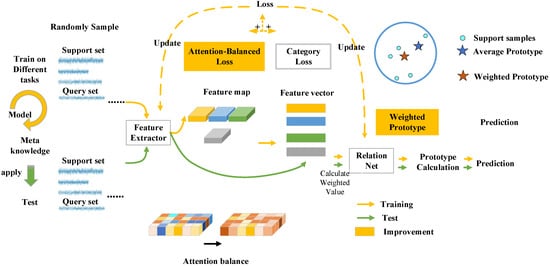
Figure 1.
Overview of Framework.
This paper is organized as follows: Section 2 introduces the task settings in meta-learning. Section 3 describes our method including attention-balanced loss and weighted prototypes in detail. Section 4 presents our experiments and results. Section 5 is a discussion of the experiments. Section 6 provides a conclusion for this article.
2. Preliminaries
This section introduces the task-based episodic training process of few-shot radar emitter signal recognition. Here, we divided the radar emitter signals owned into three datasets
, which contain categories , respectively. The training and validation sets include classes with many radar emitter signals to simulate the source data. During the training and validation stage, a large number of tasks that are regarded as few-shot problems are randomly sampled in each epoch to train and validate the model’s generalization. The test set contains the actual few-shot radar emitter signals we want to identify, so in a real-world application, the few-shot recognition problem is achieved by inputting the signals of the test set into the well-trained model directly. In order to examine the effect of models in experiments, we generated a test set that consists of classes with numbers of radar emitter signals and evaluated the performance by the average of a certain number of tasks sampled in the test set. Notice that there is no intersection between the categories of the three datasets. Additionally, each episode is composed of a support set which represents the reference signals and a query set which represents the signals to be recognized. Specifically, a support set and a query set are sampled randomly from dataset with the same N classes, where the support set contains K samples for each class with available labels, and the query set contains M samples for each class. The objective of few-shot learning is to utilize multiple episodes to allow the networks to possess metaknowledge which can generalize well on . In this work, we set N = 3 and M = 5.
The prototype concept of PN is shown in Figure 2. The network evaluates the Euclidean distance between the feature vectors of each query sample and each prototype which is calculated from feature vectors of support samples in the same class as follows:
where is the prototype of class , means the samples belong to class in this support set and is the label of the radar sample , represents the feature map of , and is the feature extractor network composed of four 1D CNN blocks.
where is the Euclidean distance between
, the prototype of class
, and the feature vector of the query sample .
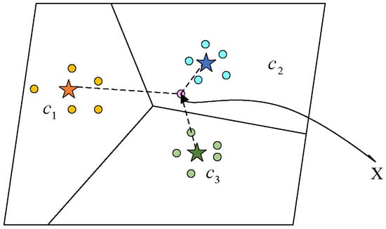
Figure 2.
The illustration of PN.
After calculating the distance, the probability distribution of the query signal is predicted by the softmax function as follows ( is the loss of PN):
3. Method
In this section, we describe our method with attention-balanced strategy and weighted prototype in order. As shown in Figure 1, the final loss function is composed of the original category loss—which is calculated by the distance between feature vectors of prototypes and query samples—and our attention-balanced loss, which is calculated by the distances between support feature maps from different classes. Furter, we weighted the support feature vectors in the same classes when K > 1 to reduce the deviation of prototypes.
The feature extractor is the same as the original PN with 1D CNN except the pool size is 4. Specifically, it contains four convolutional blocks and a flatten layer. Each convolutional block is composed of a 1D convolutional layer whose settings are 64 filters and kernel size 3, a batch normalization layer, a relu activation layer, and a 1D maxpool layer with pool size 4.
The relation net contains two convolutional blocks and two fully connected layers with units [1,16]. The composition of convolutional blocks is the same as above and the active function of each fully connected layer is relu and sigmoid, respectively. The input of the relation net is the feature vectors of two samples concatenated in depth and the output is a value with the meaning of the relationship.
3.1. Attention-Balanced Strategy
Meta-learning aims to apply generalized networks trained with the recognition of based classes to novel classes. In the field of radar emitter signal recognition, it may be difficult for the base classes to achieve comprehensive coverage to guarantee the generalization of the model obtained in the training stage as we mentioned in Section 1. This issue contributes to the result that the networks’ discriminate location learned in the training stage cannot be perfectly adaptive to the novel classes, even missing the critical location, which is important to novel class recognition. This affects the prediction and the subsequent analysis of the radar emitter systems.
To avoid this problem, we designed an attention-balanced loss composed of a distance standard deviation loss and a distance average loss, whose purpose is to balance networks’ attention in the training stage. It works by minimizing the distance standard deviation to push every position in the channel of the feature map to make the same contribution to the distinguishment of different classes and by maximizing the distance average to guarantee that the feature vectors of different classes are distinctive. In this way, the networks are supposed to pay attention not only to the location important to the base classes but also to other locations which may be critical to novel classes. The detailed calculation is as follows:
where is the distance between the feature map of sample and sample , means the samples belong to class in this query set, means the samples belong to class in this support set except class
, is the number of samples in each class in a query set, and is our attention-balanced loss.
The final loss, which is described as follows, is composed of the original class loss and our attention-balanced loss. We set as 1 and as 0.5.
3.2. Weighted Prototype
In [5], Snell defined a class’s prototype as the mean of its support feature vectors. However, in the few-shot recognition problem, the number of samples given in each class may be only 5 or even smaller. Under such a condition, one extreme sample can easily create a bias on the prototype. Additionally, the quality of the radar emitter signals we received varies due to the external environment or interference, which means the importance of each support sample to the class should also be different. As shown in Figure 3, it can be seen from (a) that the query sample belonging to class 2 will be mistakenly considered as one of class 3; as a result of this, it is closer to c3 than c2 with the average prototype calculation.
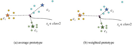
Figure 3.
Average prototype and weighted prototype.
As a consequence, it is necessary to discriminate each sample’s importance of the same class to each weighted sample, as in Figure 3b. To achieve this aim, we constructed a relation net to calculate the relation between each support sample in the same class, that is, we wanted the net to explore a way for measuring the closeness of the relationship between two support samples in the same class. The input of the relation net is two support samples’ feature vectors concatenated in the depth dimension. If two support samples are closely related, it indicates that the similarity between the two samples is high. The closer the relationship a support sample has with any other support sample in the same class, the more important the sample is to the construction of the prototype. As a result, we utilized the importance of each support sample to calculate its weight value. The detailed calculation is shown as follows:
where is the relation between the feature vector of sample and the feature vector of sample , and are support samples belonging to the same class, is the feature extractor and is the relation net, is the average of the relation between and other support samples in the same class, which represents the importance of sample , and is the weight value of sample .
To summarize, the pseudocode to the processing flow of ABPB is provided in Algorithm 1.
| Algorithm 1: Episode-based training for ABPN |
| Input: the training set Initialization: Randomly initialize model parameters , and learning rate For = 1: episode number Randomly sample N classes from the training dataset Randomly extract K samples from each of the N classes Randomly extract J samples from While Calculate weighted prototypes by Equations (10)–(12) Classify signals in to the nearest prototypes by the distance calculated in Equation (2) Calculate Loss by Equation (9) Update End while Output: Model parameters |
4. Experiments
In this section, we validate our few-shot radar emitter recognition algorithm. As we described in Section 2, first, a radar emitter signal dataset is generated and divided into a training set, a validation set, and a test set. Then, our networks presented in the previous section are trained with the utilization of the training set and validation set to obtain the generalization. Finally, the performance of the well-trained network is evaluated on the test set to examine the performance of few-shot radar emitter signal recognition. The results indicate that our algorithm possesses more advantages than other algorithms.
4.1. Dataset
Fourteen types of radar emitter signals commonly used in radar systems [25,26] are chosen in our experiments, including continuous wave (CW), linear frequency modulation (LFM) signals, nonlinear frequency modulation (NLFM) signals, multiple linear frequency modulation (MLFM) signals, double linear frequency modulation (DLFM) signals, even quadratic frequency modulation (EQFM) signals, binary phase-shift keying (BPSK) signals, binary frequency shift keying (BFSK) signals, quadrature phase-shift keying (QPSK) signals, quadrature frequency shift keying (QFSK) signals, and mixed modulations BPSK–LFM, BFSK–BPSK, BFSK–QPSK, and QFSK-BPSK. The specific parameters of the signals are shown in Table 1.

Table 1.
Specific parameters of the 14 radar emitter signals.
Due to the fact that the frequency characteristics of radar signals are obvious enough to distinguish most types of radar signals and are superior to the time–frequency spectrum in terms of time consumption, we conducted experiments with the frequency signals. The production of the dataset is described as follows:
- (1)
- First, we generate 14 types of radar emitter signals with 200 samples under each signal–noise ratio (SNR) value, which ranges from 0 dB to 9 dB with a step of 1 dB;
- (2)
- Second, we perform 2000 points fast of Fourier transform (FFT), processing the signal generated by (1). Furthermore, z-score normalization is adopted to further process the data to facilitate network optimization and reduce training time;
- (3)
- Third, we divide the generated dataset into three parts, including a training set, a validation set, and a test set. With the consideration of one-time occasionality in dataset division, three experiments are conducted to ensure the effectiveness of the test. Different divisions of the dataset are shown in Table 2.
Table 2. Different classifications of experiments.
4.2. Results
In this section, we simulated the application of MAML on radar emitter signal recognition [17] and three classical metric-based meta-learning methods including a matching network (MN) [4], PN [5], and a relation network (RN) [6] as comparison methods. The settings of [4,5,6] are the same as those in the references except for the CNN we used, which is 1D, and the setting of [17] is identical to what is described in [17]. Additionally, three sets of experiments are conducted with the datasets described in Section 4.1, and each set carries out 3-way 5-shot and 3-way 1-shot experiments with five query samples per class. Our model is described in Section 3 and the pool size is 4 under the consideration of the length of radar emitter signals being larger and maxpool layers with large size can accelerate the training process.
In the training stage, the optimizer used is an adaptive moment estimation (ADAM) with a 0.0005 learning rate and the epoch is set as 100. We choose the well-trained model with the criterion of the highest validation accuracy to test the effectiveness of the method and regard the average of 20,000 tasks randomly sampled in the test set as the final test accuracy. All experiments are implemented using the TensorFlow framework on NVIDIA GPU RTX 3090 and i9-10980XE@3.00GHz processors. Table 3 shows the results of three sets of experiments on few-shot identification.
Table 3.
Classification accuracies on few-shot recognition with different methods.
It is shown that with the application of an attention-balanced strategy and weighted prototypes, our method obtains the best performance for few-shot recognition of radar emitter signal identification in all experiments, regardless of whether the experiment pertained the 3-way 1-shot case or the 3-way 5-shot case. Furthermore, it can be noticed that the performances of our method are significantly superior to PN, the basis of which we improved on, especially for the 3-way 1-shot case, and we received an average accuracy of 94.296% of ABPN in Experiment 2, which is nearly 4 percentage points higher than that of PN. This mainly gives credit to the utilization of an attention-balanced strategy because the operation of the weighted prototype is not performed in a 1-shot case. Considering the reason the model achieves an apparent increase in the 1-shot case, which only utilizes the attention-balanced strategy, compared with the 5-shot case, which utilizes both improvements, we think it is because the model’s overfitting to base classes plays an important effect on its performance in the application of PN for few-shot radar emitter recognition and prototype bias affect little. Furthermore, due to the few samples having an adverse effect on the construction of detailed descriptions for the classification task and the learning of generalization, the 1-shot case may suffer a greater influence of the base classes’ overfitting than the 5-shot case.
5. Discussion
In this section, we have conducted ablation experiments to show the optimization enhancements of each proposed improvement to the model and fully illustrate the feasibility of the algorithms. In addition, specific discussions are carried out to further demonstrate the superiority of our modifications.
We compare PN combined with each of our proposed improvements and PN to see the contribution each improvement makes to the increase in recognition accuracy. Furthermore, PN with the LAT strategy [11] is also conducted as a comparison algorithm to verify the performance of our attention-balanced strategy. Experiment parameters and the model structure are identical, and the size of maxpool layers is 4. Table 4 shows the results of the independent few-shot validation experiments for each innovation point.
Table 4.
Ablation studies of improved and optimized on few-shot recognition.
As shown in the table, the proposed algorithms all achieve better performance in the experiments. Specifically, the attention-balanced strategy improves recognition accuracies by 0.026–2.768% and the weighted prototype contributes a 0.003–0.229% increase. It is obvious that the attention-balanced strategy effectively improves the model’s performance. As a result, the strategy enhances the model’s generalization so that the model is friendly to novel class recognition rather than only concentrating on recognition that benefits base classes only. As for the weighted prototype, it also realizes a partial boost in experiments, while it is not as apparent as the attention-balanced strategy dose. We consider it possibly due to the following reasons: the influence of the prototype bias problem is relatively small compared with the generalization problem, and the samples we generated evade extreme signals to a certain extent. In addition, it can be seen that our attention-balanced strategy achieves 0.119–2.174% higher improvement than the LAT strategy [8]. As a result, our loss function mainly focuses on adjusting the contribution of each channel in feature maps by reducing the distance deviation through the result rather than just improving the recognition accuracy of feature descriptors such as LAT.
Furthermore, to clearly demonstrate the function of weighted prototypes, figures of average prototypes and weighted prototypes are given in Figure 4. It is illustrated that weighted prototypes are much closer to the area where samples are clustered and suffer less from the extreme samples.
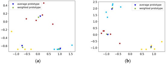
Figure 4.
Distribution of average and weighted prototypes: Two different tasks’ prototypes are shown respectively in (a) and (b). Because the feature vectors are of 448 dimensions, which are difficult to plot, we select two dimensions to plot for display. As can be seen from both figures, weighted prototypes are much closer to the area where samples are clustered.
6. Conclusions
In this paper, we proposed an ABPN for few-shot radar emitter signal recognition. Aiming at the discriminative location bias problem, we presented an attention-balanced strategy to enhance the model’s generalization. Aiming at the prototype bias problem, we introduced a relation net and a method of weighted prototype calculation to guarantee the prototypes’ rationality. The comparison results with other metric-based methods and the application of MAML on radar emitter signal recognition show the superior performance of ABPN. Further experiments and relevant discussion clearly illustrate the contribution of each of our improvements and prove the effectiveness. We also realize the shortcomings of our method in that there is no improvement on the feature extractor, which is too simple to limit the model’s ability. In future work, we hope to construct a well-performing multi-scale feature extractor to obtain more information on inputs, thereby increasing the recognition rates.
Author Contributions
Conceptualization, J.H.; methodology, J.H.; software, J.H. and X.L.; validation, J.H. and X.W.; formal analysis, J.H. and X.W; investigation, J.H. and B.W.; resources, B.W. and X.L.; data curation, J.H.; writing—original draft preparation, J.H. and X.W.; writing—review and editing, J.H., X.W. and B.W.; supervision, P.L. All authors have read and agreed to the published version of the manuscript.
Funding
This research was funded by the CETC Key Laboratory of Electromagnetic Spectrum Operation and Applied: JS20210900458.
Data Availability Statement
Data sharing is not applicable.
Acknowledgments
The authors would like to show their gratitude to the editors and the reviewers for their insightful comments.
Conflicts of Interest
The authors declare no conflict of interest.
References
- Yang, L.; Zhen, P.; Wang, J.; Zhang, J.; Guo, D. Radar Emitter Recognition Method Based on Bispectrum and Improved Multi-channel Convolutional Neural Network. In Proceedings of the 2021 6th International Conference on Communication, Image and Signal Processing (CCISP), Chengdu, China, 19–21 November 2021; pp. 321–328. [Google Scholar] [CrossRef]
- Pu, Y.; Liu, T.; Wu, H.; Guo, J. Radar emitter signal recognition based on convolutional neural network and main ridge coordinate transformation of ambiguity function. In Proceedings of the 2021 IEEE 4th Advanced Information Management, Communicates, Electronic and Automation Control Conference (IMCEC), Chongqing, China, 18–20 June 2021; pp. 716–721. [Google Scholar] [CrossRef]
- Zhang, S.; Pan, J.; Han, Z.; Guo, L. Recognition of Noisy Radar Emitter Signals Using a One-Dimensional Deep Residual Shrinkage Network. Sensors 2021, 21, 7973. [Google Scholar] [CrossRef] [PubMed]
- Vinyals, O.; Blundell, C.; Lillicrap, T.; Wierstra, D. Matching networks for one shot learning. Adv. Neural Inf. Process. Syst. 2016, 29, 3630–3638. [Google Scholar]
- Snell, J.; Swersky, K.; Zemel, R.S. Prototypical Networks for Few-shot Learning. Adv. Neural Inf. Process. Syst. 2017, 30, 4077–4087. [Google Scholar]
- Sung, F.; Yang, Y.; Zhang, L.; Xiang, T.; Torr, P.H.; Hospedales, T.M. Learning to compare: Relation network for few-shot learning. In Proceedings of the IEEE Conference on Computer Vision and Pattern Recognition (CVPR), Salt Lake City, UT, USA, 18–23 June 2018; pp. 1199–1208. [Google Scholar]
- Fort, S. Gaussian prototypical networks for few-shot learning on omniglot. arXiv 2017, arXiv:1708.02735. [Google Scholar]
- Fu, W.; Zhou, L.; Chen, J. Bidirectional Matching Prototypical Network for Few-Shot Image Classification. IEEE Signal Process. Lett. 2022, 29, 982–986. [Google Scholar] [CrossRef]
- Shao, H.; Zhong, D.; Du, X.; Du, S.; Veldhuis, R.N.J. Few-Shot Learning for Palmprint Recognition via Meta-Siamese Network. IEEE Trans. Instrum. Meas. 2021, 70, 5009812. [Google Scholar] [CrossRef]
- Zhang, X.; Qiang, Y.; Sung, F.; Yang, Y.; Hospedales, T. RelationNet2: Deep comparison network for few-shot learning. In Proceedings of the 2020 International Joint Conference on Neural Networks (IJCNN), Glasgow, UK, 19–24 July 2020. [Google Scholar]
- Huang, J.; Chen, F.; Wang, K.; Lin, L.; Zhang, D. Enhancing Prototypical Few-Shot Learning By Leveraging The Local-Level Strategy. In Proceedings of the 2022 IEEE International Conference on Acoustics, Speech and Signal Processing (ICASSP), Singapore, 23–27 May 2022; pp. 1660–1664. [Google Scholar] [CrossRef]
- Wang, Y.; Anderson, D.V. Hybrid Attention-Based Prototypical Networks for Few-Shot Sound Classification. In Proceedings of the 2022 IEEE International Conference on Acoustics, Speech and Signal Processing (ICASSP), Singapore, 23–27 May 2022; pp. 651–655. [Google Scholar] [CrossRef]
- Finn, C.; Abbeel, P.; Levine, S. Model-agnostic meta-learning for fast adaptation of deep networks. In Proceedings of the International Conference on Machine Learning; PMLR: Long Beach, CA, USA, 2017. [Google Scholar]
- Hu, Z.; Gan, Z.; Li, W.; Wen, J.Z.; Zhou, D.; Wang, X. Two-Stage Model-Agnostic Meta-Learning With Noise Mechanism for One-Shot Imitation. IEEE Access 2020, 8, 182720–182730. [Google Scholar] [CrossRef]
- Nguyen, T.; Luu, T.; Pham, T.; Rakhimkul, S.; Yoo, C.D. Robust Maml: Prioritization Task Buffer with Adaptive Learning Process for Model-Agnostic Meta-Learning. In Proceedings of the 2021 IEEE International Conference on Acoustics, Speech and Signal Processing (ICASSP), Toronto, ON, Canada, 6–11 June 2021; pp. 3460–3464. [Google Scholar] [CrossRef]
- Chen, Y.; Hoffman, M.W.; Colmenarejo, S.G.; Denil, M.; Lillicrap, T.P.; Botvinick, M.; Freitas, N. Learning to Learn without Gradient Descent by Gradient Descent; PMLR: Long Beach, CA, USA, 2017. [Google Scholar]
- Yang, N.; Zhang, B.; Ding, G.; Wei, Y.; Wei, G.; Wang, J.; Guo, D. Specific Emitter Identification with Limited Samples: A Model-Agnostic Meta-Learning Approach. IEEE Commun. Lett. 2021, 26, 345–349. [Google Scholar] [CrossRef]
- Huang, J.; Wu, B.; Li, P.; Li, X.; Wang, J. Few-Shot Learning for Radar Emitter Signal Recognition Based on Improved Prototypical Network. Remote Sens. 2022, 14, 1681. [Google Scholar] [CrossRef]
- Guo, J.; Wang, L.; Zhu, D.; Zhang, G. SAR Target Recognition With Limited Samples Based on Meta Knowledge Transferring Using Relation Network. In Proceedings of the 2020 International Symposium on Antennas and Propagation (ISAP), Osaka, Japan, 25–28 January 2021; pp. 377–378. [Google Scholar] [CrossRef]
- Liu, Q.; Zhang, X.; Liu, Y.; Huo, K.; Jiang, W.; Li, X. Few-Shot HRRP Target Recognition Based on Gramian Angular Field and Model-Agnostic Meta-Learning. In Proceedings of the 2021 IEEE 6th International Conference on Signal and Image Processing (ICSIP), Nanjing, China, 22–24 October 2021; pp. 6–10. [Google Scholar] [CrossRef]
- Wang, K.; Zhang, G.; Xu, Y.; Leung, H. SAR Target Recognition Based on Probabilistic Meta-Learning. IEEE Geosci. Remote Sens. Lett. 2021, 18, 682–686. [Google Scholar] [CrossRef]
- Wang, Y.; Gui, G.; Lin, Y.; Wu, H.-C.; Yuen, C.; Adachi, F. Few-Shot Specific Emitter Identification via Deep Metric Ensemble Learning. IEEE Internet Things J. 2022. [Google Scholar] [CrossRef]
- Che, J.; Wang, L.; Bai, X.; Liu, C.; Zhou, F. Spatial-Temporal Hybrid Feature Extraction Network for Few-shot Automatic Modulation Classification. IEEE Trans. Veh. Technol. 2022. [Google Scholar] [CrossRef]
- Xie, C.; Zhang, L.; Zhong, Z. Few-Shot Unsupervised Specific Emitter Identification Based on Density Peak Clustering Algorithm and Meta-Learning. IEEE Sens. J. 2022, 22, 18008–18020. [Google Scholar] [CrossRef]
- Wu, B.; Yuan, S.; Li, P.; Jing, Z.; Huang, S.; Zhao, Y. Radar Emitter Signal Recognition Based on One-Dimensional Convolutional Neural Network with Attention Mechanism. Sensors 2020, 20, 6350. [Google Scholar] [CrossRef]
- Yuan, S.; Wu, B.; Li, P. Intra-Pulse Modulation Classification of Radar Emitter Signals Based on a 1-D Selective Kernel Convolutional Neural Network. Remote Sens. 2021, 13, 2799. [Google Scholar] [CrossRef]
Publisher’s Note: MDPI stays neutral with regard to jurisdictional claims in published maps and institutional affiliations. |
© 2022 by the authors. Licensee MDPI, Basel, Switzerland. This article is an open access article distributed under the terms and conditions of the Creative Commons Attribution (CC BY) license (https://creativecommons.org/licenses/by/4.0/).