SLAM Overview: From Single Sensor to Heterogeneous Fusion

Abstract

After decades of development, LIDAR and visual SLAM technology has relatively matured and been widely used in the military and civil fields. SLAM technology enables the mobile robot to have the abilities of autonomous positioning and mapping, which allows the robot to move in indoor and outdoor scenes where GPS signals are scarce. However, SLAM technology relying only on a single sensor has its limitations. For example, LIDAR SLAM is not suitable for scenes with highly dynamic or sparse features, and visual SLAM has poor robustness in low-texture or dark scenes. However, through the fusion of the two technologies, they have great potential to learn from each other. Therefore, this paper predicts that SLAM technology combining LIDAR and visual sensors, as well as various other sensors, will be the mainstream direction in the future. This paper reviews the development history of SLAM technology, deeply analyzes the hardware information of LIDAR and cameras, and presents some classical open source algorithms and datasets. According to the algorithm adopted by the fusion sensor, the traditional multi-sensor fusion methods based on uncertainty, features, and novel deep learning are introduced in detail. The excellent performance of the multi-sensor fusion method in complex scenes is summarized, and the future development of multi-sensor fusion method is prospected.

1. Introduction

With the gradual introduction of intelligent robot technologies into people’s lives, their great convenience causes their demand to increase, and countries around the world are also promoting the development of an intelligent robot field. Robots can be applied to many practical scenarios: indoor sweeping robots, autonomous driving cars in the wild, underwater environment detection robots, aerial drones, and even virtual scenarios such as AR and VR, which have received extensive attention. However, this also leads to more core problems. Without high-precision positioning and mapping technology, sweeping robots cannot move autonomously and often bump into each other when placed in a room. Self-driving cars, drones, and underwater robots can easily veer off the road, causing irreparable accidents; in AR and VR, users cannot locate their position, let alone roam in the virtual scene. Therefore, SLAM technology has come into being, which can provide spatial positioning information and construct maps and virtual scenes according to its location [1].

SLAM stands for simultaneous localization and mapping [2]. Localization refers to confirming the pose of the robot and surrounding objects in the world coordinate system, and mapping refers to building a map of the surrounding environment perceived by the robot. By carrying specific sensors, the robot determines its motion trajectory through the observation of the environment without prior information of the environment, estimates its motion, and builds a map of the environment.

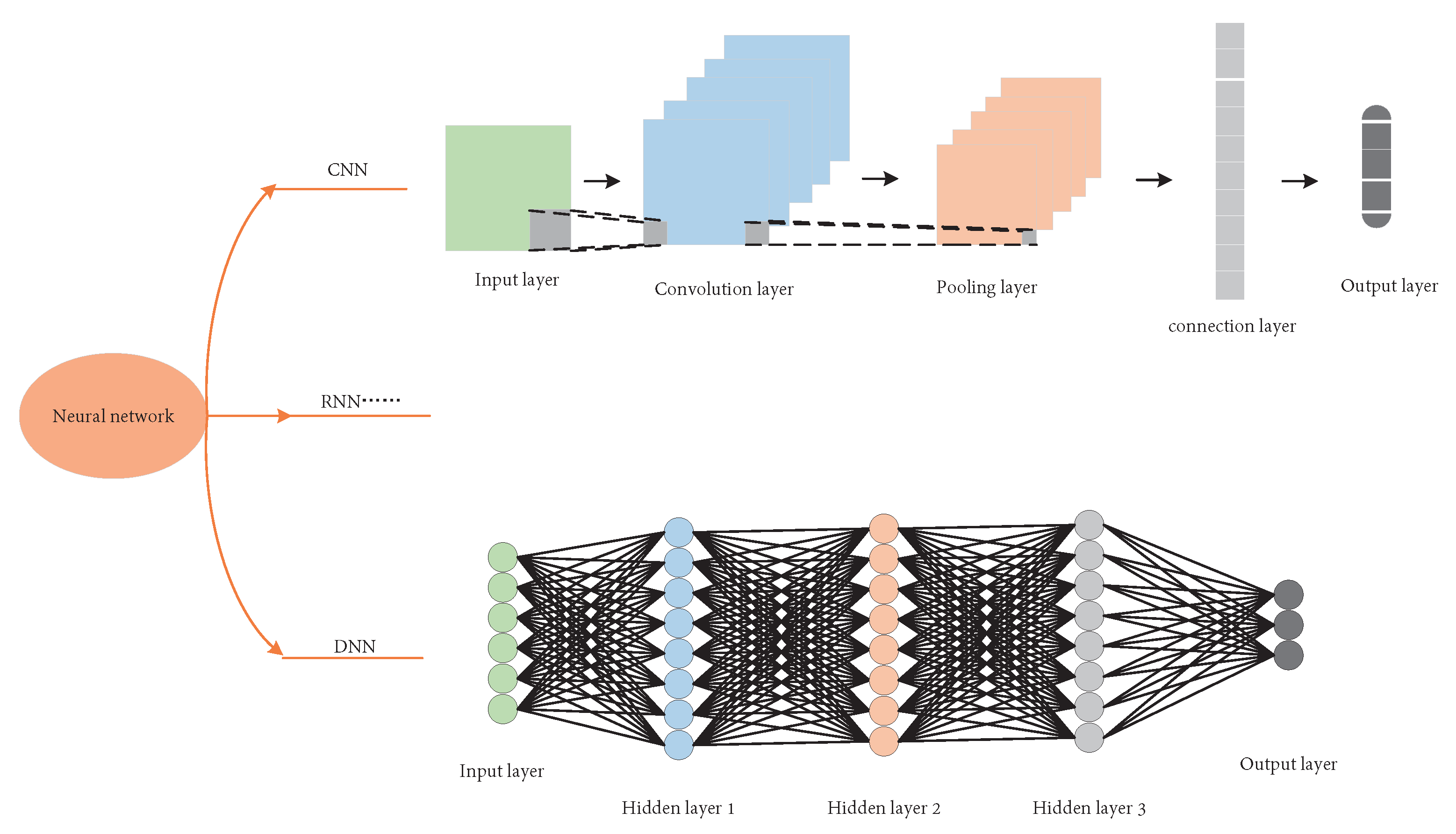
Early researchers divided SLAM into visual SLAM and LIDAR SLAM according to the different types of sensors used in SLAM technology, such as cameras and LIDAR [3]. In recent years, with the development of the computer field and the continuous exploration of this field by researchers, composite SLAM has appeared, such as VINS (IMU + visual) and RTAB-MAP (LIDAR + visual), in addition to relatively novel SLAM technologies, including CNN-SLAM (based on the semantic pattern recognition method) and DeepVO (based on the end-to-end deep learning method). In the following, this paper will outline the development history of SLAM technology from early SLAM to current SLAM technology. This paper summarizes the development of the SLAM field since 1986. From the perspective of the algorithms, the development of the SLAM field is divided into three stages. As shown in Figure 1, this paper describes the focus and contribution of SLAM in different periods from three aspects: classical model stage, machine learning and optimization stage, and deep learning stage. The following describes the basis for this article and the milestones that have been reached during these three phases. There is no absolute end to this division, and some work is still ongoing, but we made the decision to establish a crude division according to the readers’ potential research focus. If there is a mistake, the readers are welcome to correct it.

Phase 1: Classical model phase.

The probabilistic perspective of SLAM was first presented at the 1986 ICRA conference, which marked the beginning of classical SLAM. Since then, consistent probabilistic mapping has been recognized as a fundamental problem in robotics, resulting in many important papers. The original work was conducted by Smith, Cheesman, and Durrant-Whyte [2,4]. A statistical basis for describing the relationship between landmarks and dealing with the relationship between geometric uncertainties was established. At the same time, N. Ayache and O.D. Faugeras [5], J.L. Crowley [6], and R. Chatila and J.-P. Laumond [7] were the first to use the Kalman filter algorithm for mobile robot visual navigation. In 1990, R.C. Smith et al. [8] pointed out that when a mobile robot moves in an unknown environment using the correlations observed between landmarks, due to the general error of the robot’s positioning, the estimation of landmarks is necessary to correlate them with each other. Afterwards, many aspects of the SLAM problem were continuously developed. However, perhaps because of the hardware, there was a focus on the huge computational burden when the researchers determined the convergence and steady-state behavior of a map, and on the built figure relating to the consistency of solutions for a series of approximate research methods; therefore, the study of the theory of global positioning and built figures remained stagnant for a period of time [9]. SLAM achieved a conceptual breakthrough with the realization of joint localization and mapping as a convergent estimation problem. In 1995, H.F. Durrant-Whyte et al. [10] presented the structure and convergence of the SLAM problem and used the acronym “SLAM” for the first time. Their paper expounded the core structure and application fields of the SLAM problem, but there was no standard and efficient solution at the time. With the introduction of this problem, it attracted more and more scholars and research teams to carry out simultaneous localization and mapping work, especially J.J. Leonard [11] and J.A. Castellanos [12,13]. The authors of [14,15,16,17] studied SLAM applications in different environments. During this period, M. Csorba developed an important theory on convergence in [18,19], which explained the main reason affecting computational efficiency: updating the observation model based on the EKF is required to use all markers and joint covariance matrices. J.E. Guivant et al. [20] and J.J. Leonard et al. [11] carried out extensive research on the problem of low computational efficiency. In 2001, J. Neira and J.D. Tardos [21] pointed out that the standard EKF method cannot screen out the wrong landmark observation points; the global pose optimization must be carried out in the loop closure stage; and the EKF requires a definite motion and observation model and a linear assumption of the model. S.J. Julier et al. [22] studied the impact of nonlinear models on the performance of the EKF. In 2002, the FastSLAM algorithm proposed by M. Montemerlo [23] was presented, which was different from the traditional EKF-SLAM work at that time. It retained the core linear Gaussian assumption, but the adopted method was based on recursive Monte Carlo sampling and particle filtering, which demonstrated the nonlinear process model and non-Gaussian state distribution for the first time. In 2005, V.A. Sujan et al. [24] proposed an algorithm based on iterative sensor planning and sensor redundancy, which could construct a geometrically consistent environment map in an unstructured environment.

Phase 2: Machine learning and optimization.

At the beginning of this stage, the LIDAR-based method was the mainstream of SLAM research. Specifically, scholars focused on how to optimize the algorithms and how to reduce the error. At this time, the development of SLAM entered the second stage: machine learning and optimization. Based on the research results of F. Lu et al. [25] and J. Gutmann et al. [26], researchers made improvements and focused on improving the effectiveness and robustness of optimization under SLAM problems. The studies of [27,28] summarized their improvement methods. SLAM was then formalized as a problem of maximum a posteriori estimation, using factor graphs [29] to reasonably explain the interconnections between variables. The maximum a posteriori estimation method is proven to be more accurate and effective than the original SLAM filtering methods (EKF-SLAM, FastSLAM). This optimization problem is solved by continuity linearization. The current canonical forms of SLAM generally refer to maximum a posteriori estimation, factor graph optimization, graph-SLAM, and SAM (smooth mapping). The main idea of the framework focuses on pose graph optimization, where the variables to be estimated are the poses sampled along the robot trajectory, and each factor imposes a constraint on each pair of poses. In 2006, H. Durrant-Whyte and T. Bailey [30] focused on the recursive Bayesian formulation of the SLAM problem, obtaining probability distributions or estimates of absolute or relative positions of landmarks and vehicle poses. Both the source code used to evaluate SLAM algorithms and the location of real data were cited, and some key implementations in the form of state space and particle filtering were described. In 2008, J. Aulinas et al. [31] established a general classification of existing filtering strategies, such as the Kalman filter (KF), information filter (IF), unscented Kalman filter (UKF), and compressed Kalman filter (CKF), and compared their advantages and disadvantages in maps with different scenes and different numbers of landmarks. The scope of application was also presented. In 2011, G. Grisetti and R. Kummerle [32] offered a comprehensive introduction to the graph-based SLAM problem, synthesizing an effective and state-of-the-art graph-based SLAM method. A sophisticated solution based on least squares error minimization was discussed, and the structure of the SLAM problem was exploited in the optimization process.

With the rapid development of computer vision, researchers found that cameras can obtain richer information than LIDAR: compared with the point cloud data in the environment acquired by LIDAR SLAM, visual SLAM can form gray or color images. Additionally, the price of vision sensors is low, their structure is simple, the method of their installation is more diversified, and the sensors can work in both indoor and outdoor environments. However, early visual SLAM was based on filtering theory and its nonlinear error model and huge amount of calculation became obstacles to its practical landing. At this time, feature-based methods slowly appeared in the field of vision of scholars. G. Dissanayake and S. Huang [33] systematically analyzed the basic characteristics of feature-based SLAM and investigated the observability and convergence-related problems of different versions of SLAM problems. F. Fraundorfer and D. Scaramuzza [34] extensively introduced the development history of visual odometry, from offline-only work to real-time work. Feature matching, robustness, and applications were discussed. The main point feature detectors and different outlier suppression methods commonly used in VO were also reviewed. Special emphasis was placed on random sample consensus (RANSAC) and the design strategy. In 2015, R. Mur-Artal and J.M.M. Montiel [35] proposed a new feature-based ORB-SLAM system, which achieved unprecedented performance compared with other state-of-the-art monocular SLAM methods. This system can run in real time in large, small, indoor, and outdoor environments. It is robust to severe motion clutter, allows wide-baseline loops to be closed and relocated, and includes fully automatic initialization.

Phase 3: Deep learning stage.

Since 2016, with the rise in the deep learning field, researchers have found that the application of deep learning methods in computer vision can greatly alleviate the problems that are difficult to solve using traditional methods. At this current time, SLAM is in the third stage: the deep learning stage. The study of [36] summarized SLAM based on deep learning in detail and pointed out the shortcomings of traditional methods. Subsequently, SLAM research based on deep learning proliferated and achieved commendable results in LIDAR SLAM and visual SLAM. B. Bescos et al. [37] developed a visualization system based on ORB-SLAM—a dynamic object detection and background repair function. Detecting moving objects via a multi-view geometry, deep learning, or a combination of both is especially suitable in highly dynamic scenes. X. Han, H. Laga, and M. Bennamoun [38] used convolutional neural networks (CNNs) to carry out the 3D reconstruction of images, and deep learning technology to estimate the 3D shape of general objects from single or multiple RGB images. In LIDAR SLAM, C. Li et al. [39] applied a recurrent convolutional neural network (RCNN) to a mobile robot equipped with a 2D LIDAR and an inertial measurement unit to solve the problem that the accuracy greatly decreases when the rotation angle is large. D. Cattaneo et al. [40] proposed an end-to-end detection network for the loop closure detection stage of LIDAR SLAM, which detects the six-degree-of-freedom relative transformation between the current scan and the map by identifying the visited landmarks, effectively reducing the drift accumulated over time.

At the same time, inspired by deep learning methods, traditional feature- and uncertainty-based methods have also been further developed. S. Huang and G. Dissanayake [41] provided a critical review of the current theoretical understanding of the fundamental properties of SLAM problems, such as observability, convergence, achievable accuracy, and consistency, and discussed the respective application scenarios, advantages, and disadvantages of filter- and optimization-based SLAM algorithms. In 2017, the ORB-SLAM2 [42] system appeared, which can be used with monocular, stereo, and RGB-D cameras, in contrast to the previous version, with uses in loop closure, repositioning, and map reuse. At the back-end, the BA method is used to optimize monocular and stereo observations. The lightweight localization mode allows zero-drift localization during the matching process with map points. Shortly after this, C. Campos et al. [43] developed the ORB-SLAM3 system, the first system to be able to perform visual, visual inertial, and multi-map SLAM using pinhole and fisheye lens models with monocular, stereo, and RGB-D cameras, relying on MAP estimation, with significantly improved accuracy. Additionally, this system can be used during IMU initialization. Similarly, feature-based methods also have their limitations: the extraction of key points and the calculation of descriptors are very time-consuming. When features are missing, there will not be enough matching points to estimate the camera motion. To overcome these shortcomings, the direct method has been introduced, which uses the optical flow to track the motion of feature points. Direct sparse odometry (DSO) [44] utilizes a fully direct probabilistic model (which minimizes the photometric error) to perform the consistent joint optimization of all model parameters (including geometric parameters), which further improves the tracking accuracy and robustness compared to current direct and indirect methods. Besides that, there are SVO [45] and LSD-SLAM [46].

As can be seen, at present, visual SLAM and the development of LIDAR SLAM are mature, and the vast majority of the scenes presented in this article can be applied to real life, but they still have disadvantages that cannot be ignored. With visual SLAM, the disadvantage is that a lot of information is needed to obtain an accurate depth, which can lead to inaccurate positioning and tracking failure, as well as inaccurate map reconstruction. LIDAR SLAM can achieve good results both indoors and outdoors, but it is expensive, and many LIDAR systems have difficulty detecting objects at very close distances.

To this end, researchers have considered the fusion of LIDAR with cameras or other sensors, thus addressing the aforementioned shortcomings. However, there is no comprehensive summary of the current methods for multi-sensor fusion. In 2020, C. Debeunne et al. [47] summarized the related methods of LIDAR and visual fusion, but the introduction of the LIDAR and visual fusion method algorithm in this paper was too brief, and the development process of data fusion was not analyzed in detail. In 2022, X.B. Xu et al. [48] summarized the loose coupling and tight coupling methods based on 3D LIDAR, visual SLAM, and IMUs. However, their paper did not explore the development history of LIDAR and visual hardware and only summarized the data coupling method based on the SLAM system in recent years. Additionally, it did not analyze the current popular multi-sensor data fusion method based on deep learning. Therefore, it is necessary to carry out a more comprehensive analysis of the fusion of multiple sensors in the field of SLAM to help researchers and students better carry out their work. The review in this paper addresses these issues and makes the following contributions:

(1) This paper reviews the hardware development history of LIDAR and visual SLAM more comprehensively, deeply analyzes the principle of related hardware information in the field of SLAM, and summarizes the hardware brands and models of mainstream manufacturers at home and abroad.

(2) This paper uses Citespace to analyze and summarize the whole SLAM field and the fusion field and summarizes the commonly used datasets and evaluation tools in the SLAM field.

(3) This paper summarizes the fusion methods of LIDAR and visual SLAM and other sensor fusion SLAM methods from the perspectives of uncertainty, traditional features, and deep learning. To the best of our knowledge, this is the first review of fusion methods from this perspective.

This article reviews the development history of SLAM and research in this field in recent decades, as well as the major achievements. Further, this paper expounds visual SLAM, LIDAR SLAM, and their derivative methods and algorithms. In addition, this paper summarizes the research achievements of SLAM’s predecessors, and on this basis, this paper expounds visual SLAM, LIDAR SLAM, and SLAM for multi-sensor fusion. Section 2 introduces the hardware used in SLAM, and the datasets and development processes applied in recent decades; Section 3 introduces the development of using only a single sensor for localization and mapping; Section 4 introduces SLAM, which integrates vision, LIDAR, and more sensors. Section 5 concludes this paper with a summary and outlook. The overall framework of this paper is presented in Figure 2, for the readers’ convenience.

2. Related Work

2.1. Commonly Used Sensors in SLAM

In this paper, SLAM is divided into LIDAR SLAM and visual SLAM according to the different types of sensors used in the field of SLAM, as well as the use of inertial sensing units fused with LIDAR and visual SLAM to assist in the localization process of SLAM.

IMUs have a high angular velocity measurement accuracy. Their angular velocity measurement accuracy and local position measurement accuracy are higher than those of odometry. An IMU sensor contains three single-axis accelerometers and three single-axis gyroscopes, which provide self-motion information, allow the recovery of the metric scale of monocular vision, and estimate the direction of gravity, rendering absolute pitch and roll observable.

2.1.1. Hardware in Visual SLAM

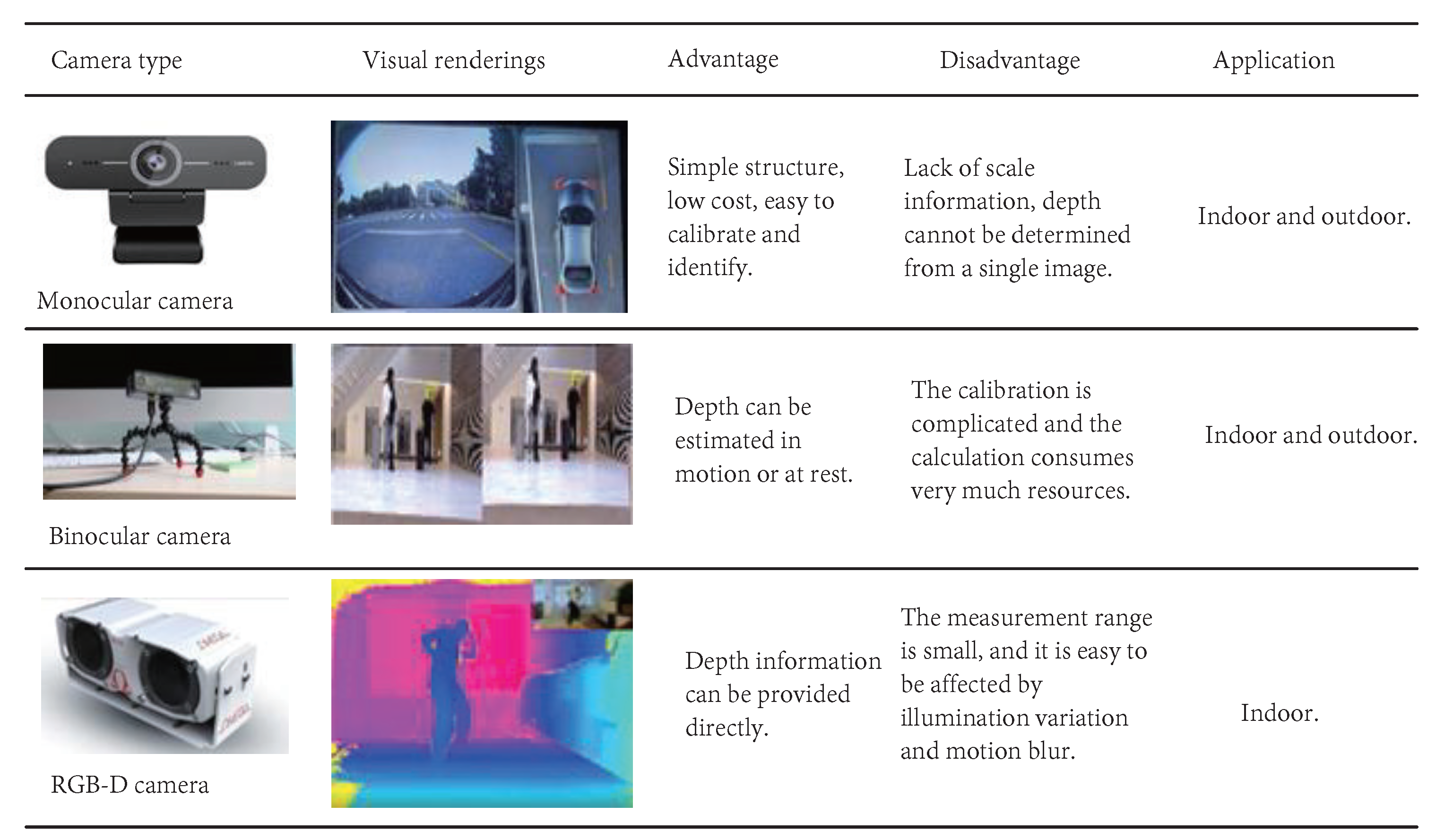
Sensors used in visual SLAM typically include monocular cameras, binocular cameras, and RGB-D cameras. Monocular cameras use only one camera for trajectory estimation and mapping. These cameras’ structure is simple, low-cost, and easy to calibrate and identify. However, the trajectory and map estimated by monocular SLAM will differ from the true trajectory and map by a factor, i.e., the scale, and this true scale cannot be determined by the image alone, which is also known as scale uncertainty. Currently, there are two main ways to solve this problem:

(1) The distance between two images is normalized, and the scale of the two frames before and after is used as the subsequent scale, which is also known as the initialization of monocular SLAM.

(2) A global estimation can be adopted, and a uniform scale can be used.

A binocular camera is composed of two monocular cameras, but the distance between the two cameras (called the baseline) is known, and the spatial position of each pixel can be estimated by this baseline. The larger the baseline distance, the greater the measurement distance. Both monocular and binocular cameras measure the relative depth of an object using epipolar geometric constraints (parallax during camera motion). Unlike monocular vision, binocular vision can estimate depth in motion as well as at rest, eliminating many of the headaches of monocular vision (the inability to determine the true size of an object in a single image; it could be a big but far away object, or it could be a very close and small object).

The disadvantages of monocular and binocular SLAM are that the configuration and calibration are more complex, the depth range and accuracy are limited by the baseline and the resolution of the binocular camera, and visual computing is very computationally expensive, which needs to be accelerated using GPU and FPGA devices to output the distance information of the whole image in real time. Therefore, under existing conditions, computational complexity is one of their main problems.

RGB-D cameras are also known as depth cameras. These cameras can detect the depth of the field distance of the shooting space, which is their biggest difference from ordinary cameras. A common color camera can see and record all the objects in the camera’s view, but the recorded data do not include the distance of these objects from the camera. Only the semantic analysis of images can tell which objects are far away and which are close to the text, but there are no exact data. Through the data obtained by the depth camera, the user can accurately know the distance of each point in the image from the camera, and the real scene can be restored without additional calculations to realize scene modeling. The pixel distance is mainly measured by infrared structured light and ToF (time of flight). In the infrared structured light principle, the camera calculates the distance between the object and itself according to the returned structured light pattern. In ToF, the camera fires pulses of light at the target and then determines the distance of the object from itself based on the time of flight (the speed of the beam is usually known) between sending and returning. The principle of the two is very similar: LIDAR obtains the distance by scanning point by point, while a ToF camera obtains the pixel depth of the entire image. Therefore, RGB-D cameras will have at least one transmitter and one receiver. RGB-D cameras construct a 3D model of the environment while estimating the camera pose. These have high accuracy in indoor scenes [49], but in outdoor environments, they are highly susceptible to illumination changes and motion blur, and long-distance tracking will lead to a large cumulative error and scale offset.

Figure 3 summarizes the respective advantages and disadvantages of the three vision sensors and the main application scenarios.

As a result of sufficient market research, this paper summarizes the current mainstream manufacturers, brands, and models of monocular, binocular, and depth cameras. The brands of monocular cameras and binocular cameras are roughly the same, because they differ only in the number of cameras, and both measure distance based on the principle of disparity. Among them, the representative companies are Leap Motion, ZED, DJI, and RGD-D, whose cameras measure distance in completely different ways from each other, which can be mainly divided into two methods: ToF and structured light. Among them, the representative companies using the ToF method are Microsoft Kinect2, PMD, SoftKinect, and Lenovo Phab, and the representative companies using the structured light method are ORBBEC, Apple iPhoneX (Prime Sense), Intel RealSense, Microsoft Kinect1, and Mantis Vision. More detailed information about the various methods is presented in

Table 1. Working principle of monocular, binocular, and RGB-D cameras, information of domestic and foreign manufacturers, and related hardware.

Camera Category	RGB-D Camera		Binocular/Monocular Camera
Operating principle	ToF (the distance is measured based on the flight time of the pulsed light from the camera to the target object)	Structured light (the camera calculates the distance between the object and itself based on the returned pattern of structured light)	Parallax (estimating the spatial position of each pixel from the distance between two cameras)
Domestic manufacturers	HIKVISION, SUNNY OPTICAL, INMOTION	ORBBEC, HJIMI, PERCIPIO	PERCIPIO, zongmu, LUSTER
Foreign manufacturers	Texas Instruments, STMicroelectronics, Microsoft	Intel, Leap Motion, STEREOLABS	PrimeSense, Intel, Heptagon
Resolution	Low, generally lower than 640*640	High, up to 2K resolution	Medium, generally 1080*720
Frame rate	Up to hundreds of frames	Usually 30 frames	Usually 30 frames
Measurement range	It can measure long distances, 0.1 m–100 m	Limited by the baseline, the farther the distance, the larger the error, generally within 2 m	0.1 m–10 m
Price	Prices range from a few thousand to a few million depending on the measurement range and frame rate size	Very cheap, thousands of dollars	The accuracy is different; the prices are different: the 1 mm-level accuracy costs USD 1000, the 0.1 mm-level accuracy costs USD 10,000, and the 0.01 mm-level accuracy costs hundreds of thousands of dollars

.

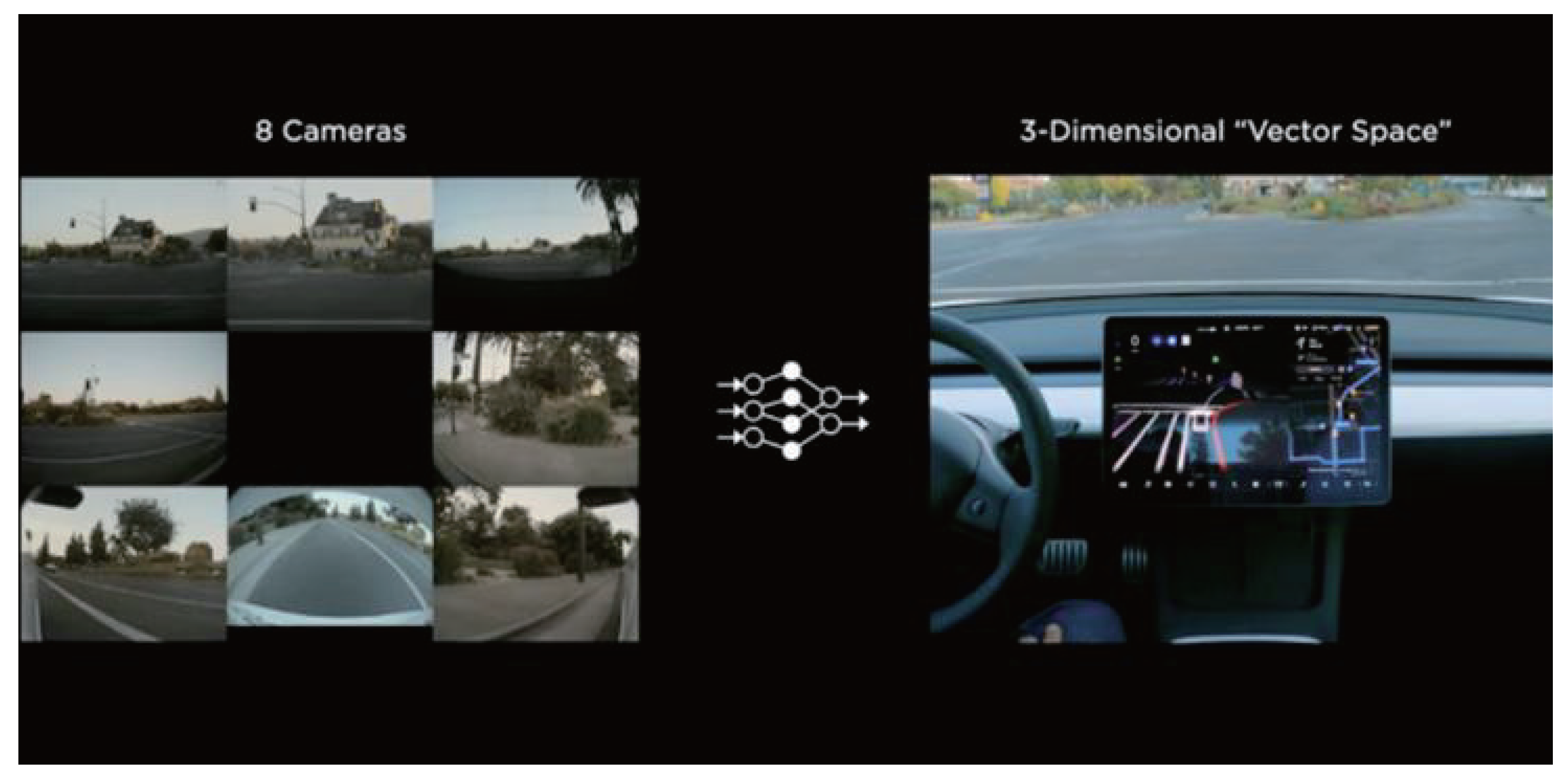
Take Tesla as an example. Tesla is a successful company in the field of pure visual SLAM. In 2021, the company released FSD Beta V9.1, the first advanced driver assistance suite using “Tesla Vision.” This vision-based autonomous driving system feeds data from eight cameras (1280 × 960 12-bit HDR 36 Hz) into a single neural network to integrate the perception of the 3D environment, as shown in Figure 4.

2.1.2. Hardware in LIDAR SLAM

In 1916, Einstein proposed the theory of the stimulated emission of light, and humans began to understand LIDAR. LIDAR is not like infrared, ultraviolet, etc., as it is a general term for a certain band of light, but it has a precise single color and single wavelength of light compared with a variety of colors and wavelengths of mixed natural light. LIDAR has high brightness, high energy, and good direction characteristics. The excellent performance of LIDAR (a dense LIDAR beam can accurately model and restore every detail of the measured object) has been gradually discovered by researchers, and it is widely used in various fields such as the military, communication, and aviation fields. However, LIDAR’s widespread adoption is attributed to a dramatic story: In 2004, the U.S. Defense Advanced Research Projects Agency launched a competition called the DARPA Driverless Car Challenge to find a solution for building driverless cars for the military. David Hall, the founder of Velodyne, modified a pickup truck with a panoramic camera to participate in the competition. Although he did not finish the race, he discovered a novel sensor in this competition: LIDAR. He then built a LIDAR that could rotate 360° and took the modified vehicle equipped with the LIDAR to participate in the DARPA Unmanned Vehicle Challenge, but the results were not satisfactory. However, their technology made them famous, and it received a lot of attention from researchers. David Hall also found business opportunities and became a professional LIDAR manufacturer, but at that time, LIDAR was mostly used in the military, meteorology, surveying, and mapping, among other professional fields, with a narrow demand, low production, and a very high price, once reaching USD 100,000.

As LIDAR has begun to be applied in civilian fields, such as unmanned driving and unmanned aerial vehicles, the huge development prospect has attracted more and more domestic and foreign enterprises. Velodyne LIDAR, Luminar, Ouster, Valeo, HESAI, HUAWEI, LIVOX, and Innovation have emerged. They began the development of vehicle LIDAR. HUAWEI has developed an infrared emitter and a ToF camera sensor by measuring the time to calculate the infrared light reflecting the depth of field. The grain race car AT128 gauge was developed at the science and technology level of long-distance half-solid-state LIDAR. At this time, various types of LIDAR are being developed, including the mechanical type, mixed solid-state type, and pure solid-state type, and the hardware cost is falling, Additionally, with the entrance of Bosch, DJI, and other giant enterprises, LIDAR is being pushed to lower prices and car standards, and the current LIDAR price has reached the lowest amount of USD 100. The process demonstration diagram of an unmanned vehicle equipped with an early mechanical LIDAR imaging system and a 4D LIDAR imaging system developed by Huawei is shown in Figure 5 for the readers’ reference.

Today’s market is gradually being divided into two different routes: pure visual and LIDAR. Among them, LIDAR SLAM is divided into 2D and 3D LIDAR. Briefly, 2D LIDAR is generally used in indoor robots (such as sweeping robots), and 3D LIDAR is generally used in the field of unmanned driving. The input and output data of 2D and 3D LIDAR SLAM are the same, but there are still some points that need to be noted. This paper summarizes the relevant information of LIDAR in Figure 6.

2.2. Development of LIDAR and Visual SLAM Algorithm

2.2.1. Development of Visual SLAM Algorithms

This paper summarizes the widely known visual SLAM algorithms. Before 2007, many scholars at the time believed that a binocular camera suite was needed to build a SLAM system. The system pioneered by Professor A.J. Davison of Imperial College London, MonoSLAM [52] broke the perception at the time, being the first case to show how to build a SLAM system using a monocular camera, building a sparse and continuous map of natural landmarks in a probabilistic framework. In the same year, a more shocking development, namely the PTAM [53] algorithm, was published by the laboratory of Oxford University, which was the first SLAM algorithm to separate tracking and mapping as two threads and also distinguish the concept of the front- and back-end in VSLAM. The algorithm uses nonlinear optimization in the back-end part, rather than the mainstream EKF filter and other filtering methods. It was a milestone at the time. In 2015, the paper on ORB-SLAM [35] was officially published, which can be regarded as an extension of the PTAM algorithm. It was the most complete VSLAM based on the feature point method at that time, and the system framework includes three threads: tracking, mapping, and loop closure. Since then, subsequent versions of the algorithm, such as ORB-SLAM2 [42] and ORB-SLAM3 [43], were published successively.

In addition to feature-based methods, direct methods also occupy an important position in SLAM. Related algorithms include LSD-SLAM [46], SVO [45], and DSO [44]. Similarly, there are related algorithms for RGB cameras. ElasticFusion makes full use of the color and depth information of RGB-D cameras, estimates pose changes through ICP, and improves the accuracy of camera pose estimation through continuous iterative optimization. Similar algorithms include DTAM, DVO, RTAB-MAP, and RGBD-SLAM-V2. This paper presents the website addresses of these algorithms in

Table 2. Common algorithms in visual SLAM.

Scenario	Author	Form of Sensor	Address
MonoSLAM	A.J. Davison	Monocular	[52]
PTAM	G. Klein and D. Murray	Monocular	[53]
ORB-SLAM2	R. Mur-Artal and J.D. Tardós	Binocular/monocular/RGB-D	[42]
LSD-SLAM	J.J. Engel et al.	Monocular	[46]
SVO	C. Forster et al.	Monocular	[54]
DTAM	R.A. Newcombe et al.	RGB-D	[55]
DVO	C. Kerl et al.	RGB-D	[56]
DSO	J. Engel et al.	Monocular	[44]
RTAB-MAP	M. Labbé	Binocular /RGB-D	[57]
RGBD-SLAM-V2	F. Endres et al.	RGB-D	[58]
ElasticFusion	T. Whelan et al.	RGB-D	[59]

for the readers’ reference.

2.2.2. Development of LIDAR SLAM Algorithm

Similarly, with the continuous development of the LIDAR SLAM field, many excellent algorithms have emerged. In 2002, M. Montemerlo et al. [23] proposed the FastSLAM algorithm, which uses a particle filter to estimate the robot pose and was the first LIDAR SLAM method to output a grid map in real time. However, in a large-scale environment, a large number of particles are needed to represent the robot pose, which seriously consumes memory. Additionally, with continuous resampling, the particle dissipation problem will gradually aggravate a situation that cannot be ignored. The Gmapping [60] algorithm was optimized based on FastSLAM, which keeps the number of particles at a relatively small value, samples the prediction distribution, and then optimizes the pose based on optimized scan matching, which solves the problem of serious memory consumption. To reduce the number of resampling iterations, resampling is only performed when the predicted distribution is very different from the true distribution, which solves the problem of particle dissipation, but this method is very dependent on odometry. Since filtering-based methods can be applied to 2D LIDAR SLAM, graph optimization-based methods can also be used. Hector SLAM was proposed by S. Kohlbrecher et al. [61], which uses the Gauss–Newton method to solve the front-end scan matching problem and does not rely on odometer data, but the drift phenomenon will occur when the robot speed is too fast and there is strong rotation. The Cartographer [62] algorithm adds the loop closure detection process and combines CSM and gradient optimization in the front-end scan matching process, but this algorithm requires a huge amount of calculation.

In the field of 3D LIDAR SLAM, J. Zhang and S. Singh [63] proposed the LOAM method, which uses 3D LIDAR to collect data, carries out scan matching based on feature points, and uses a nonlinear optimization method for motion estimation, which can be operated in real-time and has high accuracy. The authors then introduced an improved version, V-LOAM [64], which uses visual odometry to estimate pose transformation at a high frequency and LIDAR odometry to optimize the motion estimation at a low frequency and calibrate drift. This method still has high robustness when illumination changes are obvious. With the need for multi-sensor fusion, matching algorithms are needed, such as LVIO [65], LEGO-LOAM [66], and LiO-Mapping [67]. A brief overview of the relevant algorithms is presented in

Table 3. Common algorithms in LIDAR SLAM.

Age	Open Source Solution	Author	Sensor	Advantage	Disadvantage
2002	FastSLAM	M. Montemerlo [23]	2D LIDAR	Outputs a raster map in real-time	In large scenarios, memory will be seriously consumed, resulting in particle dissipation problems
2007	Gmapping	Giorgio Grisetti et al. [60]	2D LIDAR	High running speed; low LIDAR frequency requirements; high robustness	Heavy reliance on odometry; unable to adapt to drones and uneven ground areas; in the case of large scenes and a high number of particles, the consumption of resources is large
2011	Hector-SLAM	S. Kohlbrecher et al. [61]	2D LIDAR	Does not rely on an odometer	LIDAR frame rate requirements are high; can adapt to air and uneven ground areas; the optimization algorithm can easily fall into the local minimum
2014	LOAM	J. Zhang and S. Singh [63]	3D LIDAR	Does not rely on an odometer	No loop closure detection
2015	V-LOAM	J. Zhang and S. Singh [64]	3D LIDAR	High precision; the algorithm has good robustness; constant drift assumption	No loop closure detection
2016	Cartographer	W. Hess et al. [62]	2D LIDAR	The accumulated error is low; the requirement for LIDAR performance is not high	A large amount of computation
2018	LVIO	J. Zhang and S. Singh [65]	3D LIDAR	Small drift; it has good robustness under illumination, rotation, and structural degradation	The effect is not good when the feature matching is poor
2018	LeGO-LOAM	T. Shan and B. Englot [66]	3D LIDAR	When the ground points are abundant, they are relatively stable; the resulting map is sparse	The lack of a ground point is prone to collapse
2019	LIO-Mapping	H. Ye et al. [67]	3D LIDAR	Features tightly coupled multi-wire LIDAR and IMU frames	A large amount of calculation; no loop closure detection part; cumulative errors cannot be eliminated
2020	LIO-SAM	T. Shan et al. [68]	3D LIDAR	Strong stability in loop closure detection	No scan match was performed globally

for the convenience of the readers.

2.3. Evaluation Tools and Datasets

In recent decades, there have been many excellent SLAM algorithms, which have been extensively applied in the fields of autonomous navigation, mobile robots, and AR/VR. Each algorithm has its unique improvement method, and different algorithms take different amounts of time, can achieve different accuracies, and can be applied in different scenarios. Therefore, a unified evaluation tool is needed to test the performance of these algorithms on datasets. Accuracy is the most important indicator for researchers to evaluate SLAM algorithms, which includes the absolute trajectory error (ATE) and relative pose error (RPE). The relative pose error is used to calculate the difference in the pose change for the same two timestamps, which is suitable for estimating the system drift. The absolute trajectory error directly computes the difference between the true value of the camera pose and the estimated value of the SLAM system.

EVO [69] is a common tool for evaluating improved SLAM algorithms and is available for a variety of datasets. In addition to the availability of TE and RPE data, it is also possible to plot the test algorithm against the real trajectory. SLAMBench2 [70] is a publicly available software framework that evaluates current and future SLAM systems through an extensible list of datasets. This includes both open and closed source codes while using a list of comparable and specified performance metrics. It supports multiple existing SLAM algorithms and datasets, such as ElasticFusion [59], ORB-SLAM2 [42], and OKVIS [71].

Once we have the tools to evaluate the performance of an algorithm, we need to visualize the algorithm on a dataset. Common datasets used to test visual SLAM versus LIDAR SLAM are presented in the following table. The TUM dataset is collected by an RGB-D sensor, which provides indoor image sequences under different textures, illuminations, and structure conditions. According to different requirements, it is divided into TUM RGB-D [72], TUM MonoVo [73], and TUM VI [74]. TUM RGB-D contains the color and depth images of real trajectories and provides acceleration data from a Kinect sensor. TUM MonoVO is a dataset used to evaluate the tracking accuracy of monocular vision and SLAM methods, which contains 50 real-world sequences from indoor and outdoor environments, and all sequences are photometrically calibrated. The TUM VI dataset provides the criteria for evaluating visual inertial odometry, providing a highly dynamic range and photometrically calibrated images that can be evaluated in different scenes using different sets of sequences. KITTI [75] is currently the world’s largest computer vision algorithm evaluation dataset in autonomous driving scenes, which contains real image data collected in urban, rural, and highway scenes and has various degrees of occlusion. The Oxford [76] dataset contains data on a continuous stretch of road in Oxford, which contains scenes of pedestrians, vehicles, and road construction under various weather conditions. The ASL Kinect [77] dataset provides a modular ICP library based on ROS. The ASL RGB-D [78] dataset is mainly used to test the performance of robot path planning algorithms. The ICL-NUIM [79] dataset is designed to benchmark RGB-D, visual ranging, and SLAM algorithms. The VaFRIC [80] dataset can test the influence of different exposure times on camera tracking. The EuRoC [81] dataset focuses on evaluating visual inertial SLAM algorithms in real industrial scenarios.This article presents a common datasets in the SLAM field in

Table 4. Common datasets in SLAM field.

Dataset	Sensor	Environment	Availability
KITTI	RGB-D+LIDAR+GPS+IMU	Outdoor	[75]
Oxford	RGB-D+LIDAR+GPS+IMU	Outdoor	[76]
ASL Kinect	RGB-D	Indoor	[77]
ASL RGB-D	RGB-D+LIDAR	Indoor	[78]
TUM RGB-D	RGB-D	Indoor	[72]
ICL-NUIM	RGB-D	Indoor	[79]
VaFRIC	RGB-D	Indoor	[80]
EuRoC	Binocular+IMU	Indoor	[81]
TUM VI	Binocular+IMU	Indoor/Outdoor	[74]
TUM monoVO	Monocular	Indoor/Outdoor	[73]

.

2.4. SLAM Development Analysis Based on Literature Data

Since the emergence of SLAM, it has been widely used in the field of robotics. As shown in Figure 7, this paper selected approximately 6500 popular articles related to mobile robots from the past 25 years to create a keyword heatmap. The larger the circle, the more frequently the keyword appears. The circle layer represents the time from the past to the present from the inside out, and the bluer the color, the more attractive it is. The connection line indicates that there is a connection between the different keywords, where the data come from the Science Network Core collection. In this figure, circle simultaneous localization and mapping, mobile robot, motion and tracking are particularly prominent. This indicates that SLAM and mobile robots are closely combined. The development of SLAM technology constantly promotes the application of mobile robots and autonomous vehicles in complex scenes. In addition, emerging technologies such as deep learning and data association have emerged. Through these hot words, readers can learn more about hot directions in SLAM.

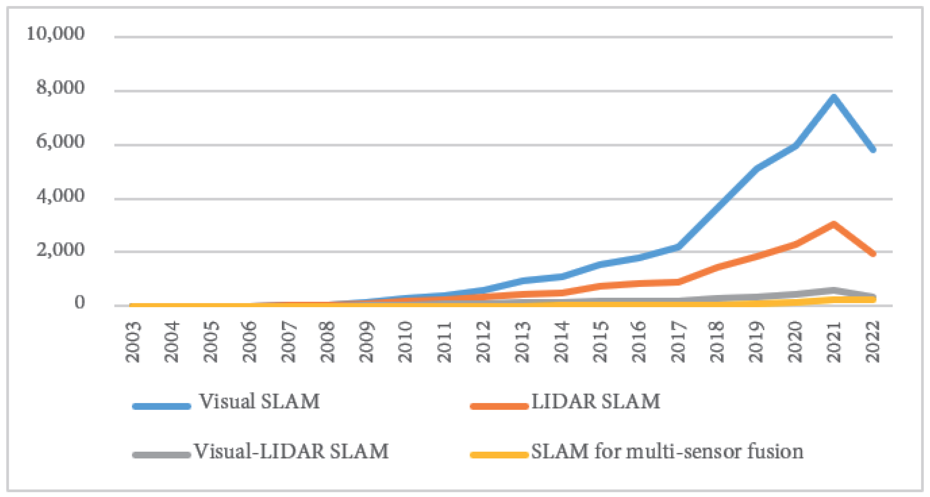
In Figure 8, this paper counts the citations of SLAM methods with a single sensor and multi-sensor fusion from 2003 to 2022, where the red and blue lines represent LIDAR and visual SLAM methods, respectively, and the gray and yellow lines represent visual-LIDAR fusion and multi-sensor fusion SLAM methods, respectively.

As can be seen in Figure 8, the number of citations of papers related to the SLAM field has rapidly increased, and the decline in 2022 is due to the data collected in the first eight months of 2022. From the published SLAM article names, SLAM is a hot topic in robotics. At the same time, the number of citations of multi-sensor fusion methods in the field of SLAM has also increased year by year, but it is still at a very low level. Therefore, the prospect of SLAM with multi-sensor fusion methods can be reasonably calculated, but the current technology is not mature enough, and there are many blank fields.

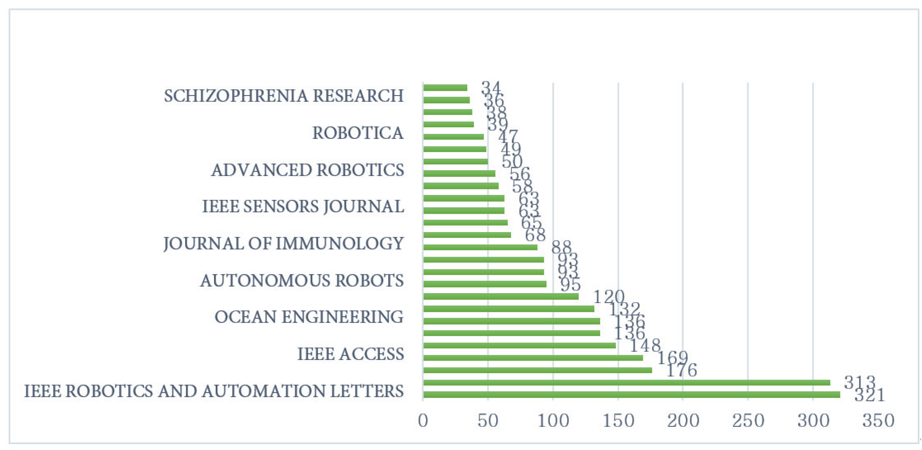
In Figure 9, the paper analyzes the publications of 25 major journal societies in the field of SLAM on Web of Science until October 2022. Only the names of some journal societies are shown in the figure. At present, the number of papers in the field of SLAM is 6959, to which IEEE Robotoics and Automations Letters and Sensors make the largest contributions with 321 and 313 SLAM publications, respectively. These statistics are enough to prove that SLAM is a hot topic right now.

2.5. Outstanding Scholars in the SLAM field

With the continuous in-depth research of scholars in the field of SLAM, many outstanding scholars and research teams have emerged successively, and their existence has set the field of SLAM on a new journey. As shown in Figure 10, this paper analyzed approximately 2000 articles between 2002 and 2022 (the data in this paper are from the Web of Science website), where the larger the font size, the higher the number of papers published by the author and the greater the attention received. Among them, Y. Liu worked on SLAM and semantic SLAM for multi-sensor fusion, and A.J. Davison is a pioneer in the field of SLAM. He first proposed the concept of SLAM and created the MonoSLAM [52] and DTAM [55] algorithms, making outstanding contributions. S. Wang continuously improved the algorithm and tried to apply RGB-D cameras to dynamic environments, achieving surprising results. Here, this article will not be listed, but interested readers can find it elsewhere.

At the same time, this paper also collected the countries of scholars from different regions and provides a simple summary to facilitate the readers’ understanding of which scholars are committed to SLAM research. As shown in Figure 11, different colors are used in this paper to represent different contributions to the field of SLAM. Here, white indicates that these regions have not contributed to the field; red indicates that the number of papers contributed by these regions is less than 100; yellow indicates that the number of papers contributed by these regions is in the range of 100 to 300; green indicates that the number of papers contributed by these regions is in the range of 300 to 900; and blue indicates that the number of papers contributed by these regions is above 900. From the figure, it can be concluded that scientists in China, the United States, and the United Kingdom have made largest contributions to the field of SLAM.

3. Single-Sensor SLAM

3.1. Visual SLAM

The eyes are the main source of human access to external information, and visual SLAM has similar characteristics. It can obtain large amounts of redundant texture information from the environment and has strong scene recognition ability [82]. For example, two billboards with the same size but different contents cannot be distinguished by the LIDAR SLAM algorithm based on the point cloud, but visual SLAM can easily distinguish them. This brings incomparable advantages in relocation and scene classification. At the same time, visual information can be easily used to track and predict dynamic objects in the scene, such as pedestrians and vehicles, which is crucial for applications in complex dynamic scenes. In addition, the projection model of vision can theoretically make objects at infinite distances enter the visual picture, and under a reasonable configuration (such as binocular cameras with a long baseline), it can be used to locate and map large-scale scenes.

C. Cadena et al. [83] proposed a classical visual SLAM framework, as shown in Figure 12, which is mainly composed of four modules: front-end (usually feature extraction and data association in visual odometry), back-end (usually data optimization and map update), loop closure detection, and mapping [84].

Early visual SLAM was based on filtering theory, and its nonlinear error model and huge amount of computation have always been the bottlenecks of its development. Since recent years, with the progress of nonlinear optimization theory with sparsity, camera technology, and computing performance, the real-time running of visual SLAM is no longer a dream. Generally, a visual SLAM system consists of four parts: front-end, back-end, loop closure detection, and mapping. The most important of these are the front-end and back-end, which this article will focus on, while the other two parts will be briefly outlined.

3.1.1. Front-End (Visual Odometer)

The front-end mainly estimates the platform position and attitude by analyzing the changes between camera [85] frame sequences through visual odometry. At present, the algorithms of the front-end part are mainly divided into two categories: feature point methods and direct methods [86].

The front-end based on the feature point method has been considered the current mainstream method because of its stability, insensitivity to illumination, and dynamic objects. Researchers usually regard corners, edges, and pixel blocks in images as image feature points. The method of feature extraction involves confirming the correspondence between the corners in different images according to their positions, to obtain the motion trajectory of the object. Before 2000, many corner extraction algorithms appeared successively, such as Harris [87], FAST [88], and GTFF [89]. However, the method of feature matching using corner points often has many errors. For example, when the camera rotates or the distance changes, the original corner points may be invalid. Therefore, the researchers designed SIFT [90], SURF [91], ORB [92], and other more stable local image features to solve this problem. In

Table 5. Commonly used feature extraction algorithms in SLAM.

Algorithm	GTFF	Harris	FAST	SIFT	SURF	ORB
Year	1994	1988	2006	2004	2008	2011
Speed	Medium	Slow	Fast	Slow	Medium	Fast
Advantage	The Harris algorithm is improved, and the ability of corner extraction is stronger	The feature points extracted by this algorithm have rotation invariance and affine invariance	The comparison of pixel brightness greatly accelerates the process of image feature extraction and includes the description of the scale and rotation	The changes in illumination, scale, and rotation in the process of image change are fully considered	Feature extraction and description are more efficient and have scale invariance	ORB is 100 times faster than SIFT and 10 times faster than SURF
Disadvantage	There is no scale invariance	There is no scale invariance	The repeatability of feature points is not strong, and the distribution is not uniform	It is computationally intensive and requires the use of a GPU	Compared with the SIFT algorithm, the accuracy and robustness are decreased	It has no rotation invariance and scale invariance and is sensitive to noise

, this paper summarizes the main performances of these feature extraction algorithms.

After extracting the feature points, the most critical step is to match the feature points, to prepare for the subsequent pose estimation and optimization. The simplest feature matching method is brute force matching, i.e., matching a moment of the image feature point with the current moment of all of the image feature points, which measures the descriptors of similar degrees between two characteristics of the distance, but when there is a high number of feature points, the violent match will produce a significant amount of calculation, which is unable to meet the demands of real-time performance. M. Muja and D.G. Lowe et al. [93] proposed a new fast approximate nearest neighbor (FLANN) algorithm, which uses hierarchical k-means trees and greatly reduces the application search time.

Finally, the matched feature point pairs are obtained; at this time, the camera motion can be estimated according to the point pairs. According to the different sensors used in visual SLAM, the following three cases can be observed: when the camera is a monocular camera, 2D pixel coordinates can be obtained, and the motion can be estimated by the method of epipolar geometry; when the camera is a binocular or RGB-D camera, the distance information is obtained, and researchers usually use the iterative closest point (ICP) [94] algorithm to solve the motion estimation of two sets of 3D points; when one group is 3D and the other is 2D, this can be solved using the PnP [95] method. The schematic of a camera performing pose estimation is presented in Figure 13.

Although the feature point method occupies the mainstream position in the front-end part, it still has many shortcomings: the extraction of feature points and the calculation of descriptors are very time-consuming. Extracting only feature points does not represent all the information in the image and may neglect the most important part of the image. Camera motion may not be estimated when features such as texture are missing. To solve the above problems, the researchers developed a direct method, which is similar to the optical flow method based on the gray invariant assumption, which can estimate the camera motion according to the brightness information of the pixels [96], completely avoiding the calculation of feature points and descriptors. Compared with the sparse map constructed by the feature point method, the direct method can construct sparse, semi-dense, and dense maps according to the needs of different scenes. Similarly, the direct method is also updated iteratively. Since the first use of the direct method of DTAM [55] in 2011, it has achieved excellent performance in the accurate reconstruction of maps. Since then, LSD-SLAM [46], SVO [54], DSO [44], and other algorithms have appeared. The accuracy of motion estimation and robustness in low-texture regions and blurred images are further improved by these algorithms.

In

Table 6. Commonly used feature extraction algorithms in SLAM.

Method	Feature Point Method	Direct Method
Conception	The camera motion is estimated according to the extracted and matched feature points, and the camera motion is optimized by minimizing the projection error	The camera motion is estimated according to the pixel brightness information, and the method of minimizing photometric error is used in the optimization step
Advantage	The feature points themselves are not sensitive to illumination, motion, and rotation and are relatively stable	Semi-dense and dense maps can be built and work as long as there is light and shade variation in the scene
Disadvantage	Computing feature points and descriptors consumes a large amount of computing resources and cannot be used when feature points are missing	It is easily affected by illumination changes, and the discrimination is not strong when there are few pixel blocks
Applicable scenes	Richly textured scenes	Feature-missing scenes, such as white walls and empty corridors

, for the convenience of the readers, the differences between the direct method and the feature point method are summarized.

3.1.2. Back-End Optimization

The early back-end optimization problem was a state estimation problem. In the first series of papers, researchers called it “estimation of spatial state uncertainty”, which also reflected the core of the SLAM problem: the estimation of the spatial uncertainty of the moving subject itself and the surrounding environment. Additionally, in the process of using the sensor, it will inevitably have a certain noise, and it will be affected by factors such as temperature, humidity, and light. Therefore, one has to use a method to reduce the error of the whole framework. State estimation theory is used to express the uncertainty of localization and mapping, which is called maximum a posteriori probability estimation (MAP).

At present, the back-end optimization methods of SLAM are mainly divided into two types: filtering methods represented by extended Kalman filtering and nonlinear optimization methods represented by graph optimization.

Filter-based methods have been widely used since 2008 when Csorba et al. developed an important theory of convergence in [18,19]. Despite having convergence capability, they are not computationally efficient because the update of the observation model of the EKF needs to use all the markers and joint covariance matrices. J.E. Guivant et al. [20] and J.J. Leonard et al. [11] started some work on improving the computational efficiency during this period. In 2001, J. Neira et al. [21] pointed out that the EKF method in the standard form is very fragile to the incorrect association between landmark observations, leading to the “loop closure detection” problem. In addition, the EKF requires clear motion and observation models and linear model assumptions. S.J. Julier and J.K. Uhlmann [22] studied the impact of nonlinear models on the performance of EKF applications. Since then, various filters and their improved algorithms have been developed, such as the IF [24], IKF [97], UKF [98], particle filter [99,100,101], and SWF [102]. Some algorithms are improved based on the EKF. For example, ref. [103] proved that all processes related to the motion perception update cycle of EKF-SLAM can be carried out in a time linear relationship with the number of map features, and an improved algorithm was proposed to reduce the complexity of the calculation. The study of [104] proposed monocular SLAM based on the EKF, which combined RANSAC and a random list to process images and showed excellent performance in dealing with complex indoor environments, occlusion, and sudden motion.

Later, researchers found that, although the BA optimization method included a large number of feature points and camera poses, it constructed a sparse map and did not produce a huge amount of computation. With the publication of [105], real-time visual SLAM based on graph optimization was proposed. Subsequently, G. Grisetti and R. Kummerle [32] offered a comprehensive introduction to the graph-based SLAM problem, synthesizing an effective and state-of-the-art graph-based SLAM method. An advanced solution based on least squares error minimization was discussed, and the structure of the SLAM problem was exploited in the optimization process. Since then, researchers gradually discovered the excellent real-time performance of nonlinear optimization algorithms. Compared with the method based on filtering, with the increase in the number of landmarks on the map, the state quantity of this method increases in a square series, and the huge amount of calculation means that the whole SLAM system is unable to run in real time. With the continuous improvement of graph optimization algorithms, the current mainstream hot spot of SLAM research is almost based on graph optimization.

3.1.3. Loop Closure Detection

The robot returns to the origin after a period of movement, but its position estimate does not return to the origin due to drift. At this time, it is necessary to match the position estimate with the origin position to let the robot know that it has been to this place; such an event is called loop closure detection [30]. Loop closure detection aims to reduce the drift accumulated during exploration by matching past keyframes with the nearest keyframes, which is verified by calculating a rigid transformation that aligns matching points between keyframes [106], and finally optimizing the trajectory to reduce the error accumulated by the trajectory. Researchers usually use visual similarity to evaluate the relationship between current camera images and past camera images. Visual similarity can be computed using global image descriptors, such as those presented in [107,108], or local image descriptors, such as those presented in [109]. In recent years, visual similarity cycle detection using local image descriptors has received extensive attention, and one of the most successful methods is based on the bag-of-visual-words model [110,111,112].

The loop closure detection step can greatly improve the accuracy and robustness of the whole SLAM system, and in some cases, researchers place systems with only a front-end and local back-end under visual odometry, and systems with loop closure detection and a global back-end under SLAM.

3.1.4. Mapping

Mapping refers to the process of building a map to understand the environmental information, find the optimal path in the current map, or search for an object on the map. According to the different scenarios of the object, the complexity of the selected map is different, which can be mainly divided into a sparse map, semi-dense map, and dense map.

If a sparse map is established, the general SLAM algorithm can be realized. However, building semi-dense and dense maps comes with a lot of computation. Both of them calculate the depth of each pixel by matching points and triangulating them. Sparse maps usually only need to calculate a few hundred points in 640*480 = 307,200 (the lowest pixel case), while dense reconstructions need to calculate the depth of almost all points, a difference of hundreds of times. Generally, a depth camera using active depth measurements such as ToF and structured light is better, but the active light source is not suitable for outdoor and large scenes, since it is susceptible to illumination interference and has a relatively small ranging range. When the pose of each frame is obtained, there are two basic methods to build the image:

(1) The simplest method is to not track the movement of feature points between frames so that there is no need for inter-frame matching, and all points are directly back-projected to the 3D space to form a point cloud. The point cloud processing method is used to remove duplicate points and noise points. This method requires that the pose is relatively accurate and the drift is small.

(2) The second method is to track the movement of points between frames, which requires feature matching. For monocular and binocular cameras, after the relative poses of the two frames are known, the matching process can be accelerated through epipolar line searching and block matching. The depth of each pixel can be obtained by triangulating the matching between the two frames. Multiple frames may see the same point, and the depth filter can use a filtering method or a nonlinear optimization method. The filtering method is less computationally intensive, as opposed to constantly calculating the depth between two frames and then updating the depth. However, the BA method can be used for the nonlinear method, but the calculation is large. Because the number of dense points is large, the calculation of BA is large and the front-end uses the computing resources. Considering the computing power, the filtering method may be more appropriate, since the matching and depth calculation of each point block are relatively independent, which can be accelerated using a parallel method.

3.2. LIDAR SLAM

LIDAR SLAM is derived from earlier range-based localization methods (such as ultrasound and infrared single-point ranging). The emergence and popularization of LIDAR have made the measurement faster, more accurate, and more informative. The object information collected by LIDAR presents a series of scattered points with accurate angle and distance information, which is called a point cloud. Usually, by matching and comparing two point clouds at different times, the LIDAR SLAM system calculates the distance of the relative movement of the LIDAR and the change in the attitude and completes the localization of the robot itself [113].

The LIDAR range measurement is more accurate, the error model is simple, the operation is stable in an environment other than direct bright light, and the processing of the point cloud is relatively easy. At the same time, the point cloud information itself contains direct geometric relationships, which makes the path planning and navigation of the robot intuitive. The theoretical research of LIDAR SLAM is also relatively mature, and the landing products are more abundant.

The LIDAR SLAM framework is the same as the visual SLAM framework, which is usually divided into four modules: front-end scan matching, back-end optimization, loop closure detection, and mapping. In the following, the basic concepts of these four modules will be roughly introduced.

Front-end scan matching is the core step of LIDAR SLAM. The work content is to know the pose of the previous frame and estimate the pose of the current frame using the relationship between adjacent frames. The front-end scan matching can generate the pose and map in a short time, but due to the inevitable error accumulation, back-end optimization is required, which involves the optimization of odometry and map information after long incremental scanning matches. Loop closure detection is responsible for reducing the drift phenomenon of the global map by detecting loop closure, to generate a consistent global map. The map-building module is responsible for generating and maintaining the global map.

3.2.1. Front-End Scan Matching

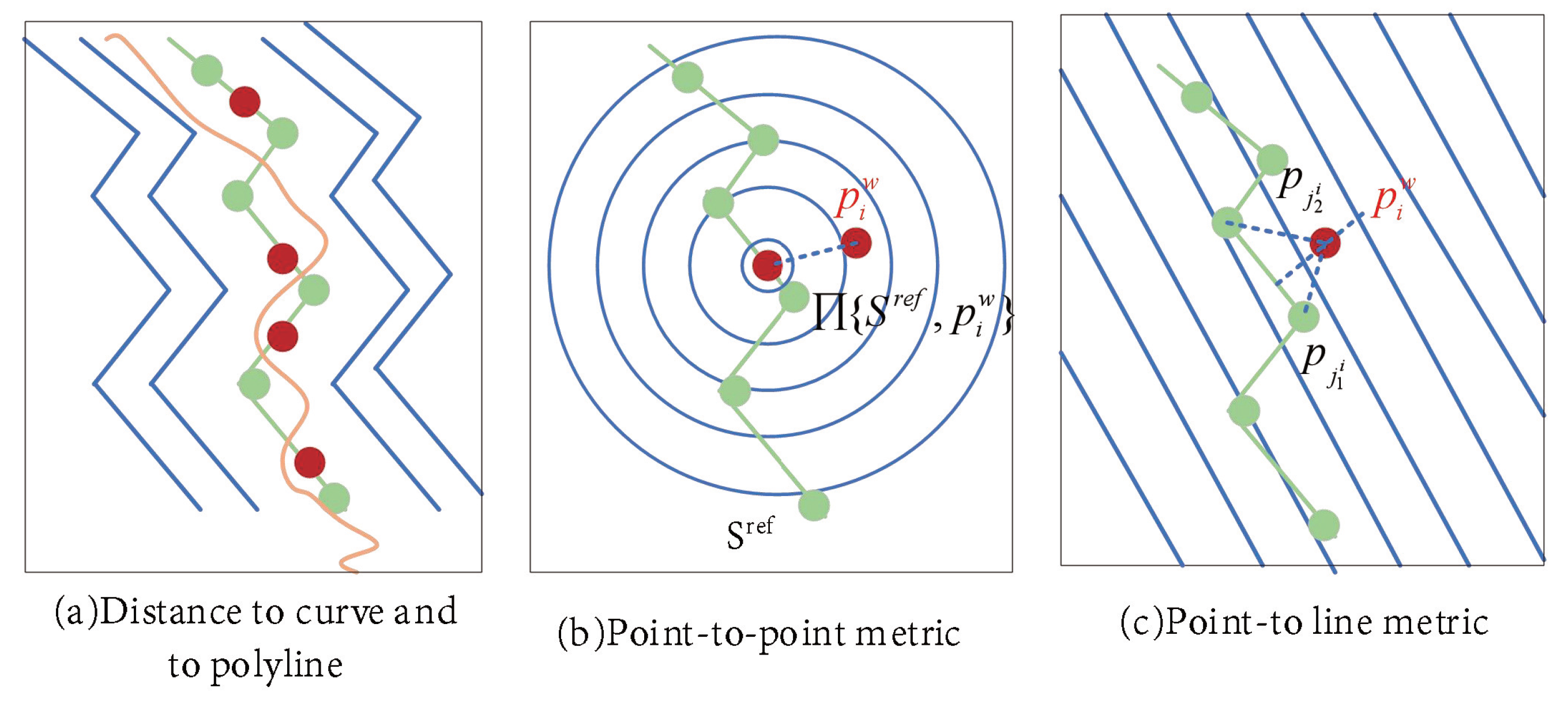
Front-end scan matching is the core step of LIDAR SLAM. The work content is to know the pose of the previous frame and estimate the pose of the current frame using the relationship between adjacent frames. In simple terms, it is the mathematical calculation process of transforming point cloud data in two or more coordinate systems into a unified spatial coordinate system. The coordinate transformation of the space can be determined by three types of parameters: scale, rotation, and translation. The ICP [114] algorithm can merge point cloud data under different coordinates into the same coordinate system, which is essential to find a rotation matrix R and a translation matrix T, and then realize the alignment matching conversion between two points. However, its disadvantage is also obvious: it consumes a lot of computing resources when performing matching between points. Additionally, it depends on the initial value. When the initial value is bad, the number of iterations increases. For large initial errors, incorrect iteration results may occur. Pl-ICP [115] is an improved ICP algorithm, and its schematic diagram is shown in Figure 14. Compared with the point-to-point registration of the ICP algorithm, the PL-ICP algorithm uses point-to-line registration.

Because PL-ICP is a second-order convergence algorithm, it is faster and more accurate than ICP’s first-order convergence algorithm, but the algorithm also requires accurate initial values. There is also a matching method between points using polar coordinates provided by LIDAR PSM [116]. In 2010, K. Konolige et al. [117] proposed a pose graph optimization method for constructing and solving linear subproblems, which effectively reduces local errors.

3.2.2. Back-End Optimization

The front-end scan matching can generate the pose and map in a short time, but because of the inevitable cumulative error, back-end optimization is required, which involves the optimization of odometry and map information after long incremental scanning matches. Similarly, the back-end optimization step also requires the use of filter-based SLAM methods and graph-based optimization SLAM methods. The process of robot SLAM is as follows: the robot is controlled to reach a pose, and then the observation is recorded; however, the observation data are usually used to deduce the pose, so the Bayesian formula is introduced. The Bayesian filter estimates the probability distribution rather than the specific value, and it is mainly divided into two processes: prediction and correction. The particle filter method can realize recursive Bayesian filtering through a non-parametric Monte Carlo simulation method, and its representative algorithm is Gmapping [60]. This provides an effective method for analyzing nonlinear dynamic systems, which can be applied in many fields such as target tracking, signal processing, and automatic control. The method based on graph optimization finds an optimal pose between each node and minimizes the error value between the prediction and observation by constructing a pose graph, and its representative algorithms are Cartographer [62] and Karto-SLAM [117].

3.2.3. Loop Closure Detection and Mapping

The loop closure detection steps of LIDAR SLAM and visual SLAM are roughly the same, so this paper will not repeat them here. However, this step of LIDAR SLAM is more complex than that of visual SLAM due to the repetition of 3D structures in the environment and the fact that LIDAR scanning uses geometric descriptors such as lines, planes, and spheres to perform matching between scans. Although the feature-based method [118] has greatly improved the processing speed and accuracy, it is still difficult to run the scan matcher in real time during each scan. Therefore, W. Hess et al. [62] applied the sliding window method to scan matching, cyclically detecting the current pose and its nearby region over a window of fixed frames. At present, the main methods of loop closure detection are scan-to-map, map-to-map [63], branch-and-bound, lazy decision, and CSM+ gradient optimization [62]. Through loop closure detection, the drift phenomenon of the global map is reduced to generate a consistent global map. The mapping module is responsible for generating and maintaining the global map. However, in the actual environment, many tricky problems are often encountered, such as degraded environments (empty corridor), dynamic updating of the map (positioning error when the map is updated), and dynamic environment localization (the influence of people, cars, and other moving objects).

3.3. Summary

In Section 4, the front-end, back-end, loop closure detection, and mapping steps of LIDAR SLAM and visual SLAM were generally explained. The two used different types of sensors. Although there are many similarities between the approximate positioning and mapping processes, the algorithms used by them are completely different. Since the development of LIDAR SLAM and visual SLAM in recent decades, both of them have relatively matured and have their advantages and disadvantages in different fields: LIDAR SLAM builds a map of high accuracy, has no accumulated error, and can be directly used for navigation and positioning, but it is expensive, and cannot fully utilize the environmental texture information. Visual SLAM can work both indoors and outdoors and has high accuracy under rich texture information, but the accuracy of the constructed map is low and there is a certain cumulative error. However, by combining the two, they have great potential to learn from each other. For example, visual SLAM works stably in dynamic environments with rich textures and can provide very accurate point cloud matching for LIDAR SLAM, while the precise orientation and range information provided by LIDAR will exert more power on correctly matched point clouds. In an environment with severely insufficient illumination or a lack of texture, the localization work of LIDAR SLAM makes it possible for visual SLAM to record scenes with little information. In this paper, it was found that the fusion method of visual and LIDAR SLAM or various other sensors is better able to adapt to complex situations and has great development prospects; therefore, this paper will describe the current existing fusion methods of different sensors in detail in the next section.

4. SLAM for Multi-Sensor Fusion

4.1. Visual Inertial SLAM

Visual SLAM algorithms have made significant breakthroughs in recent decades and can operate stably and robustly in many scenarios. However, when low-quality images are generated by fast camera movements and different light levels, current visual sensors cannot achieve good results [119]. IMU-assisted sensors, compared to odometers, have higher angular velocity measurement accuracy and higher local position measurement accuracy. When the camera moves fast, the IMU can obtain clear images of dynamic objects, and at the same time, when the speed is slow, the camera can correct the cumulative error generated by the IMU [120]. The complementarity of the two greatly improves the performance of SLAM. Moreover, due to the low price and convenient use of vision sensors and IMU sensors, more and more scholars are beginning to pay attention to them [121]. At present, according to whether the image feature information is added to the state vector, visual inertial fusion methods can be divided into tight coupling and loose coupling [122]. Loose coupling means that the IMU and the camera estimate their motion separately and then fuse their pose estimates. Tight coupling involves firstly fusing IMU and camera states, then jointly constructing motion and observation equations, and finally performing state estimation [123]. Figure 15 is a schematic of loose and tight coupling.

4.1.1. Loosely Coupled Visual Inertial SLAM

Loose coupling means that the motion estimations of the IMU and the camera are performed and then the pose estimation results of the two modules are fused. The update frequency of the two modules is inconsistent, and there is a certain amount of information exchange between the modules. J.M. Falquez et al. [124] proposed an effective loose coupling method to fuse the RGB-D camera and IMU sensor information and obtained good experimental results. Although the implementation process of loose coupling is simple, errors are often generated during the fusion process, so there has not been much in-depth research.

4.1.2. Tightly Coupled Visual Inertial SLAM

Tight coupling means that the state of the IMU and the state of the camera are merged to construct the motion equation and observation equation and then the state estimation is performed. The scale measurement information of the IMU can be used to assist the scale estimation in the vision sensor. The tight coupling method makes full use of the visual and inertial measurement information, which can obtain higher attitude estimation accuracy, but it also brings a greater amount of computation and a more complex implementation process. Over decades of development, researchers have divided tight coupling into filtering-based and graph-based optimization methods, and the algorithms and core processes used by them are detailed in the following.

In 2007, A.I. Mourikis and S.I. Roumeliotis [125] derived a real-time visual inertial model MSCKF based on the EKF, which is able to represent the geometric constraints that arise when viewing static features from multiple camera poses. The addition of 3D feature positions to the filtered state vector is avoided so that the computational complexity only grows linearly when the number of features grows. Compared with using only vision sensors, the proposed algorithm has higher estimation accuracy while obtaining rich environmental information. It can operate stably and reliably in indoor, outdoor, and other environments where GPS signals are unreliable, and the two sensors have the advantages of having a low cost, a low weight, and low power consumption, which have allowed the visual inertial navigation method to become the first choice of fusion method. Another commonly used filtering method is ROVIO [126], which only uses a monocular camera and achieves accurate and robust tracking performance by directly judging image blocks with different pixel intensities. Three-dimensional landmark positions are estimated based on the current camera pose, and the framework does not require any initialization process and can be directly applied to UAVs (multi-rotor UAVs).

A method based on the graph optimization of IMUs with binocular camera integration, OKVIS [71], has been proposed in order to reduce the complexity of the algorithm and improve efficiency. This algorithm applies the linearization and marginalized keyframes of the nonlinear optimization problem. Even though the method is more computationally demanding, compared with the filter method, it has higher precision and better performance. However, none of the above three methods have a loop closure detection module. When running for a long time, the continuous accumulation of errors will lead to the obtained global information being unable to be used for back-end optimization. In 2018, the VINS-Mono [127] algorithm successfully solved this problem. This algorithm used a tightly coupled nonlinear optimization method to fuse feature observations with IMU measurements to achieve relocation with minimal computation and performed global pose map optimization to reduce the cumulative error. In 2021, the latest ORB-SLAM algorithm, ORB-SLAM3 [43], was published, which can be applied to all current visual sensors and is the most complete open source library for visual, visual inertial, and multi-segment SLAM. It depends on the maximum a posteriori probability (MAP) estimation, even during the initialization of the IMU, and can also run in real-time indoor and outdoor scenes. It was the first algorithm to use the height of the parallax algorithm stage according to the keyframes to reuse the global information system, in contrast to the most advanced algorithm, which greatly improved the accuracy.

This paper compares several representative VI-SLAM frameworks, and it can be seen that the current mainstream VI-SLAM implementation methods are dominated by tightly coupled optimization methods. Compared with the loose coupling method, the tight coupling method that combines the IMU state and the camera state for state estimation has higher accuracy. Since the filtering-based method is a Markov method, it cannot consider the relationship between the state at a certain time and the state at all previous times. At present, it is generally believed that the optimization-based method will obtain more accurate results when the computing resources are sufficient. However, the filter-based method is still an effective method in situations where computing resources are limited or the mobile robot pose trajectory is relatively simple. The commonly used VI-SLAM algorithms are summarized in

Table 7. Commonly used feature extraction algorithms in SLAM.

Visual Inertial SLAM Algorithm	Applicable Sensor Types	Coupling Method	Front-End	Back-End	Loop Closure	Mapping	Reference
MSCKF	Monocular/binocular	Tightly coupled	FAST+Optical Flow	EKF	No	Sparse	[125]
ROVIO	Monocular	Tightly coupled	FAST+ Optical Flow	EKF	No	Sparse	[126]
OKVINS	Binocular	Tightly coupled	Harris+BRISK	Optimization	No	Sparse	[71]
VINS-Mono	Monocular	Tightly coupled	Harris+ Optical Flow	Optimization	Yes	Sparse	[127]
ORB-SLAM3	Monocular/binocular /RGB-D/ pinhole/fisheye	Tightly coupled	ORB	Optimization	Yes	Sparse	[43]

for the readers’ reference.

4.2. Comparison between LIDAR SLAM and Visual SLAM

This paper will elaborate on the application scenarios, localization and mapping accuracy, cumulative error problem, sensor cost, algorithm difficulty, computational requirements, and multi-computer collaboration of both LIDAR SLAM and visual SLAM.

(a) Application scenarios

In terms of application scenarios, the application scenarios of visual SLAM are much richer. Visual SLAM can work in both indoor and outdoor environments. However, the high dependence on light makes it impossible to work in the dark or in some untextured areas. At present, LIDAR SLAM is also used in indoor and outdoor mapping and navigation. However, in extreme weather such as rain, snow and fog, the performance is poor, the amount of data collected is too large, and the price is very expensive.

(b) Localization and mapping accuracy

In static and simple environments, LIDAR SLAM localization is generally better than that of visual SLAM, but in large-scale and dynamic environments, visual SLAM shows better results because of its texture information. In map construction, the accuracy of LIDAR SLAM is high, and the accuracy of the RPLIDAR series constructed by SLAMTEC can reach approximately 2 cm. Visual SLAM, such as the common version, also uses a lot of Kinect depth cameras (ranging from 3 to 12 m), and the accuracy of map construction is approximately 3 cm; therefore, the accuracy of the map constructed by LIDAR SLAM is generally higher than that of visual SLAM and can be directly used for positioning and navigation.

(c) Cumulative error problem

In general, LIDAR SLAM lacks the ability of loop closure detection, and it is difficult to eliminate the cumulative error. However, visual SLAM uses a lot of redundant texture information, and loop closure detection is easier. Even if the front-end accumulates a certain amount of error, the error can still be eliminated by loop closure correction.

(d) Sensor cost

LIDAR comes in many classes and costs more than vision sensors. The most expensive outdoor long-range multi-line LIDAR, such as Velodyne, is often hundreds of thousands of dollars, while the high-end long-range planar LIDAR for outdoor use, such as SICK and Hokuyo, is about tens of thousands of dollars. Indoor applications are widely used at the middle and low ends of the close-range planar LIDAR, which also costs thousands of dollars; the price is equivalent to the more high-end industrial-grade cameras and sensor chips. The cost of LIDAR is likely to drop significantly after mass production, but there is still a big question mark over whether it can be brought down to the level of comparable cameras.

(e) Algorithm difficulty

Due to its extensively developed research and relatively simple error model, LIDAR SLAM has a lower threshold in the algorithm. Some open source algorithms have even been incorporated into the ROS system and become standard configurations. In contrast, with visual SLAM, first of all, image processing itself requires deep knowledge, and map construction based on nonlinear optimization is also a very complex and time-consuming computational problem. After optimizing and improving the existing visual SLAM framework in the actual environment, such as adding an illumination model, using feature points extracted by deep learning, and using monocular and binocular fusion views, the algorithm threshold of these technologies is also much higher than that of LIDAR SLAM.

(f) Computational requirements

There is no doubt that the computational performance requirements of LIDAR SLAM are substantially lower than those of visual SLAM. Mainstream LIDAR SLAM can run in real-time on an ordinary ARM CPU, while visual SLAM requires more powerful quasi-desktop CPU or GPU support. However, the industry also sees a huge opportunity in this, and the market for ASICS customized for visual processing is already emerging. A good example is Movidius, which is owned by Intel. Intel has designed a special architecture for image, video, and deep neural network processing, and achieved the throughput of desktop-level GPUs at watt-level ultra-low power consumption. DJI’s Genie 4 series products use this type of dedicated chip to realize high-speed and low-power visual computing, which provides the basis for UAV obstacle avoidance and near-ground scene navigation.

(g) Multi-machine collaboration

Visual SLAM is mainly passive detection, and there is no multi-robot interference problem. However, LIDAR is actively launched, which may cause interference when there are many robots. In particular, the wide use of solid-state LIDAR may make the scene full of signal pollution, which affects the effect of LIDAR SLAM.

4.3. LIDAR and Visual SLAM Fusion Method

For decades, many methods in the field of LIDAR and visual SLAM technology have flourished, but they all have their limitations, as they are easily affected by external factors; therefore, more and more researchers are focusing on the integration of the two methods. By combining the depth of the accurate LIDAR estimation and the powerful features of the camera tracking ability, this type of fusion will have many advantages. The fusion of LIDAR and visual SLAM will produce a large cumulative error in high-speed motion. Therefore, inertial sensing units with a low price and excellent performance have become the first choice to make up for this defect; thus, three types of sensor fusion methods have slowly emerged. Although the fusion between multiple sensors complements the advantages of different sensors on the surface, it involves the fusion between different algorithms in essence and further shows the advantages of the algorithms through the sensors. Based on the current papers on existing fusion methods, this paper will analyze the fusion of multiple sensors from the methods based on uncertainty, traditional features, and deep learning.

4.3.1. Fusion Methods Based on Uncertainty

Uncertainty-based methods are usually used in 2D visual–LIDAR fusion SLAM. At present, there are three mainstream methods: Kalman filter (KF), particle filter, and graph-based algorithms and their derivatives. The Kalman filter and particle filter are two different implementations of the Bayesian filter. The Kalman filter is mainly responsible for the forecasting and updating of two parts, but it cannot satisfy the demand of the nonlinear problem; therefore, researchers have developed an extended Kalman filtering (EKF) method. This method has achieved good effects in mid- and small-scale scenes, but when it comes to large maps, it leads to a huge amount of computation. The unscented Kalman filter (UKF) is a good solution to nonlinear problems. However, the above KF and its variants can only deal with the case of a Gaussian distribution, and when facing the case of an arbitrary distribution, the use of the KF will bring larger errors. The method based on a particle filter solves the problem of the arbitrary distribution of multiple samples. A region with a larger number of particles in this method has a higher probability. Graph-based SLAM, on the other hand, finds the relationship between poses by minimizing the sum of squared variances.

(a) A fusion method based on the KF and particle filter

In 2006, P. Newman et al. [110] mounted a LIDAR and camera simultaneously on a mobile robot for the first time, and the LIDAR acquired the local geometry of the environment, which was used to incrementally construct a 3D point cloud map of the workspace. Data fusion was performed using standard EKF equations, and this observation was applied to the state vector. In the process of loop closure detection, the camera sequence is used for detection, and then the local LIDAR scanning is used again to process the image of the loop closure detection, which effectively eliminates the error generated by the loop closure detection process, but the huge amount of calculation is still difficult to solve. In 2009, F. Malartre et al. [128] developed a perception strategy system combining visual and LIDAR SLAM. By adding LIDAR data to the EKF, the drift of visual SLAM was reduced, and the density-controlled digital elevation map (DEM) was quickly recovered. In 2010, F. Sun et al. [129] assumed that the sensor noise obeyed a Gaussian distribution and used the EKF to estimate the minimum mean square error of the system state. Visual data and LIDAR data with the same corner features were fused, and the active detection strategy was adopted to improve the accuracy of SLAM and obtain more 3D map information.

The fusion method of the two has slowly matured, and some scholars have gradually deployed it in mobile robots, autonomous vehicles, and drones. In the process of the continuous improvement of the algorithm, excellent performance that cannot be achieved by a single sensor has been obtained.

In 2007, L. Iocchi et al. [130] used a particle filter to estimate the displacement between local maps for the mapping problem of large indoor environments. They mainly used a binocular camera to measure plane displacement, supplemented with 2D LIDAR data, which cooperated with high-precision IMU sensors to successfully construct a low-cost 3D map. The study of [131] used LIDAR data as the input of a binocular vision system and applied this system to a complex intersection scene, vehicles, and other dynamic risk levels as the output of the object, using a particle filter to solve the location problem (each particle corresponds to a vehicle location, using LIDAR data to compute the probability of each particle). This method obtained good detection effects and further shows the broad prospect of different types of sensor fusion, which has attracted the widespread attention of researchers. The multi-sensor fusion of UAVs has made breakthrough progress. In 2013, J. Collier et al. [132] used SIFT and variable dimension local shape descriptor (VD-LSD) to train the bag-of-words model of LIDAR and visual sensors based on the FAB-MAP algorithm and performed position recognition on a UAV. Regardless of poor lighting conditions or low-texture scenes, it has good recall and accuracy, but when the UAV flies too fast, it can easily lead to feature tracking failure. Figure 16 shows the multi-sensor fusion framework based on the FAB-MAP algorithm, for the readers’ convenience.

To address this problem, D. Magree and Johnson [133] used visual- and LIDAR-assisted navigation. The navigation architecture was based on EKF filters to provide sensor updates for the UAV, coupled at the scan and point correspondence levels, which reduced the impact of the fuzzy geometry generated by the rapid UAV flight. Additionally, this led to the Monte Carlo LIDAR-based SLAM system and its vision application in scan matching. S. Wang et al. [134] improved the Monte Carlo localization (MCL) method and applied it to a robot’s pose estimation procedure. This paper proposed a localization algorithm based on 2D LIDAR and 3D point clouds from a 2D structure to generate the 2D LIDAR alignment. With this algorithm, the data and map can be located in the robot’s positioning at the same time as the local map scale.

The traditional fusion method coarsely fuses LIDAR and visual SLAM and achieves good results. By more finely selecting different types of sensors for fusion, the feasibility of producing better results has been confirmed by more and more researchers. S. Huh et al. [135] deployed a monocular camera, LIDAR, and an inertial sensor on an unmanned aerial vehicle (UAV) using visual markers to calibrate the camera and LIDAR information and, based on the EKF, developed a real-time navigation algorithm, even without any a priori knowledge about the environment. E. Lopez et al. [136] improved the then-advanced monocular visual SLAM methods (LSD-SLAM and ORB-SLAM) to develop a SLAM system that integrates different visual, LIDAR, and inertial measurements using the EKF, which optimizes 6D pose estimation using the EKF, where local 2.5D maps and footprint estimates of robot positions can be obtained, improving the ability of low-cost commercial aviation platforms to build pose and environment maps in real-time on board. Y. Bi et al. [137] fused a depth camera and LIDAR and deployed them on a UAV. Hector SLAM was used to determine the relative position and orientation of the UAV, and the Gauss–Newton method was used to find the best transformation between the current scanning and mapping. This system can carry out positioning, mapping, planning, and flight in unknown indoor environments. The accurate landing of visual targets can be achieved, and all real-time calculations can be performed on the aircraft. V. De Silva et al. [138] solved the problem of fusing the output of light detection, LIDAR, and wide-angle monocular camera sensors in free-space detection by first spatially aligning the output of the sensors and then using the Gaussian process (GP) regression resolution matching algorithm to interpolate the missing data with quantified uncertainty. This data fusion method significantly improves the perception of unmanned and mobile robots. B.P.E. Vasquez et al. [139] installed a LIDAR, camera, and radio frequency identification (RFID) system on the mobile robot Doris and improved the positioning accuracy of the robot in a real environment through the EKF. It can be located only using sensor fusion and a semantic map, without mapping the whole environment by creating a point cloud map. SLAM does not need to be used. One study even put forward a bolder idea to apply SLAM technology to the simulation experiment of spacecraft landing on the moon [140]. This study combined LIDAR and monocular camera images to eliminate the error caused by scale uncertainty for the landing problem of spacecraft. The unscented Kalman filter (UKF) was used to provide state estimates based on inertial and star-tracking camera data at various stages of the spacecraft reaching the moon. A visual localization algorithm based on 2D–3D point correspondence and LIDAR distance was proposed, which can be initialized without systematic errors compared with only using optical navigation.

At present, fusion algorithms have been able to run stably on UAV and mobile robots, but there are still many problems that cannot be ignored, such as the large amount of calculation, complex process of mapping, and low accuracy of positioning. To solve these problems, researchers carried out a large number of experiments and made a lot of improvements to the front-end odometry, back-end optimization, loop closure detection, and mapping steps.

The fusion methods of front-end odometry mainly include those presented in [64,141,142,143]. The study of [64] combined visual and LIDAR odometry and proposed an online self-motion estimation method, V-LOAM. At high frequencies, self-motion is estimated by visual odometry, and at low frequencies, motion estimation and drift correction are improved by LIDAR odometry. Accurate and robust motion estimation can be achieved even when moving at high speed and the illumination changes dramatically. Additionally, this method can use different types of ranging sensors: for example, it can improve the positioning accuracy of fisheye cameras with serious distortion caused by large viewing angles.

The study of [143] developed a low-cost inertial positioning system of binocular vision combined with the multi-state constraint Kalman filter (MSCKF), a visual inertial odometer (VIO), and LIDAR information provided by a 3D map, which greatly improved the performance of the standard visual inertial odometer and reduced the positioning error system’s acceptable range. The study of [143] proposed a new method of fusing visual and LIDAR data in odometry. Visual maps of LIDAR voxel maps and map points were constructed, and the maps were integrated into the odometer measurement residuals to eliminate any errors caused by assigning the LIDAR depth to non-corresponding visual features. A large number of geometric residuals obtained by LIDAR were used instead of a single linearized residual. This greatly accelerated the iterative optimization of a similar Levenberg–Marquardt algorithm and obtained a more accurate pose estimation.

The study of [142] proposed a fully automatic end-to-end method based on the 3D–2D joint correspondence mask (CoMask), which can directly estimate the extrinsic parameters with high accuracy. The genetic algorithm was combined with the Levenberg–Marquardt method, which can solve the global optimization problem without any initial estimation. The general framework of the study is presented in Figure 17, wherein different colors are used to represent different steps to facilitate a better understanding by the readers.

High-precision mapping requires very rich information, and the rich texture information brought by the visual algorithm has great advantages in relocation. The information carried by the LIDAR point cloud is not deeply mined in this paper. In the high-end long-range multi-line LIDAR, the returned point cloud contains not only the direction and range information, but also the reflectance information of the target point. When the number of lines is large and dense, the data composed of reflectance information can be regarded as a type of texture information. Once this information is integrated into the high-precision map, the high-precision map can seamlessly switch between the two forms of point cloud and texture, which is also the research direction of some foreign teams [144].

In 2017, M. Shin et al. [145] proposed a registration method of point cloud images fused with LIDAR, an inertial sensing unit, and a camera. The SLAM method used was LOAM. By combining the odometry information obtained by the LIDAR and the 3D position of the selected image feature points, the information of the co-located positions in these two maps was extracted, and the accurate estimation of the rigid transformation between the origin of each mapping was realized. In the same year, M. Chen et al. [146] used 2D LIDAR to realize real-time 3D mapping through visual inertial fusion attitude estimation, real-time conversion from the point cloud to the world frame in pose estimation, and the accurate motion estimation of the robot through IMU-assisted visual SLAM based on the EKF. Subsequently, Z. Zhu et al. [147] proposed a visualization method based on 3D LIDAR SLAM, which uses LIDAR to provide pose and undeformed point cloud information for visual keyframes and simultaneously detects and corrects the loop closure detection. Compared with the original LOAM system, the accuracy is improved, and the motion drift generated by pose estimation is effectively reduced. The great potential of LIDAR point cloud information has attracted the attention of more and more researchers who have begun to try to use point cloud information in combination with other information. By using photometric image registration with a geometric point cloud, K. Huang et al. [148] proposed a direct LIDAR–visual measuring method process, using different sensors’ output information combined with a graphic image block with a single-plane pixel alignment formula to calculate the accurate motion estimation between frames, providing accurate projections of obstructions. Experiments on the KITTI dataset produced consistently registered colored point clouds. G. Zhou et al. [149] proposed a visual localization algorithm combining points and lines. Using the most advanced simultaneous localization and mapping algorithms at that time (such as LIO-SAM, LVI-SLAM, and Fast-LIO), 2D lines in the image could be extracted online, and 3D lines in the 3D LIDAR map could be extracted offline. Sparse 3D points are obtained by visual odometry, and their poses are constantly corrected by minimizing the reprojection errors of 2D–3D lines and 3D–3D points. Finally, zero-drift positioning can be achieved. Various researchers have tried to add point cloud information to the direct method and achieved amazing results. J. Qian et al. [150] proposed a new direct odometry method: the image data obtained by the vision sensor are combined with the sparse point cloud obtained by the LIDAR with the relative attitude as the prior. With this method, the positioning and mapping of a UAV with high accuracy and robustness are realized. W. Wang et al. [151] proposed a direct visual–LIDAR fusion SLAM framework, which includes a frame-by-frame tracking module, an improved sliding window-based refinement module, and a parallel global and local search loop closure detection (PGLS-LCD) module, and combines the bag-of-visual-words (BoW) and LIDAR iris features for location recognition. Finally, a high-precision real-world trajectory and point cloud maps can be generated. The framework diagram for generating high-precision point cloud maps using direct methods is presented in Figure 18 for the readers’ convenience.

However, correspondingly, point cloud information is easily affected by illumination, and different sensors have different viewpoints, which are difficult to make consistent in the process of extraction. To address this issue, A. Gawel et al. [152] proposed a framework that uses structural descriptors to match LIDAR point clouds to the sparse visualization of key points, which is not affected by the viewpoint and illumination changes of the sensor. The framework contains two independent pipeline inputs: LIDAR–inertial sensing unit data and visual inertial sensing unit data. When constructing the structural descriptor, the two types of data are fused to carry out feature matching, which can adapt to different environments. J. Mo and J. Sattar [153] proposed a SLAM method for location recognition using 3D LIDAR descriptors: a LIDAR sensor is used for the location recognition of 3D points obtained from stereo visual odometry. This system has higher robustness when the environment changes dramatically, and in the process of position recognition, the accuracy and computational efficiency are better than those of the traditional 2D method.

In the stages of loop closure detection and back-end optimization, the connection between them is usually considered simultaneously. In 2016, Q. Wu et al. [154] presented recursive Bayesian filters, which can handle arbitrary distributions using multiple samples. Through this method, they completed the calibration of 2D LIDAR and a panoramic camera, used the visual loop closure detection method to assist 2D-SLAM, registered the panoramic camera image with the point cloud, and obtained a 3D map with RGB-D information. This method solves the positioning problem in indoor scenes without GPS signals, and in relatively flat outdoor scenes. In the same year, R.O. Chavez-Garcia et al. [155] proposed a complete perception fusion architecture based on an evidence framework (the architecture includes three main sensors: radar, LIDAR, and camera), which uses a Bayesian filter for state prediction. The authors addressed the problem of moving object detection and tracking by integrating composite representations and uncertainty management and carried out tests in real driving scenarios, drastically reducing the number of false detections and misclassifications. S.H. Chan et al. [156] developed a method for the robust positioning of lightweight indoor SLAM. Compared with the traditional feature matching method, the algorithm uses a path-matching method, curvature filter, and pyramid filter to find the basic matrix between the different trajectories and can be applied to any type of general SLAM fusion architecture. Even with cheap sensors, the fusion method has reasonably high localization accuracy and sufficiently robust navigation. Z. Jin et al. [157] used the particle filter method to introduce a FastSLAM method that fuses a visual stereo image and 2D LIDAR data. By providing a priori mapping, the submaps obtained by the particle filter were compared with each other, which effectively eliminated the particles with large differences and made the algorithm converge quickly, providing easier access to high-definition maps. When tested on the KITTI dataset, compared with the popular ORB SLAM, the estimated trajectory was closer to the ground truth. Y. Tao et al. [158] proposed a SLAM algorithm for a multi-sensor information fusion model based on the EKF, which uses Bayesian inference and joint probability density estimation on each frame of fixed time to fuse LIDAR RBPF-SLAM and monocular vision information and has high positioning accuracy in actual scenes.

Similarly, direct methods are also widely used in loop closure detection and back-end optimization, and in 2018, great breakthroughs were achieved in this direction. R. Giubilato et al. [159] solved the scale ambiguity problem of monocular vision by fusing the range data of the LIDAR altimeter in the monocular vision odometry framework. Using the keyframe-based tracking and optical flow mapping algorithm, the distance data were used as the scale constraint between keyframes, and the optimization algorithm based on iSAM2 was applied to the back-end trajectory optimization and map estimation, which can eliminate the scale drift before the loop closure detection process. Y. Kim et al. [160] proposed a lightweight monocular vision localization algorithm to match the depth of the stereo disparity map to the 3D LIDAR map. Similar to the method of compensating for drift in the LSD-SLAM method, this paper applied the depth residual minimization algorithm to camera pose estimation, which can be applied to urban environments with weak GPS signals. Y. Shin et al. [161] proposed a camera–LIDAR sensor system using a direct method, which uses a sliding window method in pose estimation to avoid local horizontal drift. Global horizontal consistency is maintained using an appearance-based place recognition module and a pose graph optimizer. This system verifies the advantages of the direct method: it has obvious advantages in the process of fusing low-resolution cameras and sparse LIDAR data. However, more consideration is needed in the case of large changes in lighting conditions and fast-moving objects. In 2020, ref. [162] proposed a direct visual-to-LIDAR SLAM framework combining light detection, LIDAR ranging, and a monocular camera for sparse depth measurement, jointly optimizing each measurement under multiple keyframes to realize the direct utilization of sparse depth. This study addressed the unavailability of traditional keyframe-based methods in sparse-depth scenes. This method achieves robust SLAM results even with extremely sparse depth measurements (eight rays), but it is not applicable to the case of poor illumination changes. The proposed DVL-SLAM framework is presented in Figure 19.

(b) Graph optimization-based fusion method

In addition to using direct methods, graph optimization methods can also be used to determine the robot’s position. A.L. Majdik et al. [163] regarded speeded-up robust features (SURF) features as environmental landmarks and tracked the displacement of these landmarks between different positions of the robot. The cross-use of visual mapping and LIDAR mapping systems can achieve efficient localization and autonomously filter out detected landmarks. S. Houben et al. [164] abstracted LIDAR SLAM at different stages into a thin interface only connected to the map construction process, proposed a fast and simple labeling method that can effectively detect and decode, and provided a graph optimization method that can seamlessly and continuously integrate its location information in the map. G. Jiang et al. [165] proposed a new SLAM framework based on graph optimization considering the fusion of cheap LIDAR and vision sensor data. In this framework, a cost function was designed to process both scanning data and image data, and the bag-of-words model with visual features was imported into the loop closure stage. A 2.5D map containing visual features and obstacles was generated, which is faster than a traditional grid map. L. Mu et al. [166] proposed a graph-optimized SLAM method. Based on the unscented Kalman filter (UKF), four sensors including LIDAR, an RGB-D camera, an encoder, and an IMU were combined for joint positioning, which effectively improved the accuracy of loop closure detection and made the map more refined. S. Chen et al. [167] studied the back-end of LIDAR and visual SLAM and constructed a method based on loop closure detection and global graph optimization (GGO). In the main stage, the geometric features and visual features of LIDAR were used, and the bag-of-words (BoW) model describing visual similarity was constructed in the auxiliary stage. The loop closure detection and graph optimization performance were significantly improved.

At this time, for the front- and back-end optimization, loop closure testing, built figure, etc., various versions of the fusion algorithm, compared with only using a single-sensor algorithm, have obtained good effects and shown more advantages and the great potential of sensor fusion; therefore, there is an indication that the multi-sensor fusion method is also applicable to the complete process of SLAM. Inspired by the loose coupling and tight coupling methods of visual sensors and IMUs, researchers are also attempting to use loose coupling and tight coupling methods throughout the whole SLAM process to make full use of the respective advantages of different sensors.

(c) Fusion method based on loose coupling

At first, researchers focused on multi-sensor loose coupling methods. In 2017, M. Yan et al. [168] proposed a loosely coupled visual–LIDAR odometry method combining VISO2 (second version of visual odometry) and LOAM (LIDAR odometry and mapping), which utilizes the complementary advantages of different sensors to reduce the number of limited scenes. They demonstrated reasonably high accuracy even in situations where environmental texture was repeated and shape features were not prominent, but scenes with high-speed motion and lack of color and shape features still presented challenges. In 2020, multi-sensor loose coupling approaches achieved significant breakthroughs, with researchers applying them to mobile robots and various harsh environments. A multi-sensor fusion state estimation framework for legged robots was proposed by M. Camurri et al. [169] whose core is the extended Kalman filter (EKF), which fuses IMU and leg odometry sensing for attitude and velocity estimation and simultaneously uses visual sensors and LIDAR to correct motion drift in a loosely coupled manner. The performance is reliable when the robot moves for a long distance, but it is not suitable for situations where the movement speed is too fast. P. Alliez et al. [170] developed a SLAM system equipped with dual LIDAR, an IMU, a GPS receiver, and camera sensors for emergencies in the military and civilian fields. The information of each sensor is fused using the loose coupling method. The visual part is based on the ORB-SLAM algorithm, and the LIDAR part is based on the error-state Kalman filter (ESKF); the two cooperate through pose sharing and relocation and can even operate stably in harsh environments. Subsequently, in another paper [171], the same authors fused more types of sensors and proposed a real-time indoor/outdoor positioning and offline 3D reconstruction system by fusing visual–LIDAR–inertial GPS, which is based on the KF and performs a loosely coupled fusion method between the LVI-SLAM method and GPS positioning. In the case of GPS failure, dark environments, and smoky scenes, the signal can be transmitted by radio, and the localization is more accurate than that of the existing technology. To allow the readers to better understand the loose coupling method of four-sensor fusion, the general framework is presented in Figure 20 for reference.

(d) Fusion method based on tight coupling

In contrast with the previous loosely coupled fusion methods based on the Kalman filter, now, the hot spot in the academic community is tightly coupled fusion based on nonlinear optimization. For example, fusion with IMUs and real-time mutual calibration allows the LIDAR or visual module to maintain a certain positioning accuracy when maneuvering (violent acceleration and deceleration and rotation), which prevents tracking loss and greatly improves the stability of positioning and map construction.

In 2019, Z. Wang et al. [172] proposed a robust and high-precision visual inertial LIDAR SLAM system, which combines the advantages of VINS-Mono and LOAM and can effectively deal with scenes of sensor degradation. The visual inertial tight coupling method is used to estimate the motion attitude, and the estimated value of the previous step is refined through LIDAR scan matching. When one of the links fails, the tracking motion can still be continued. T. Wang et al. [173] fused sensors such as LIDAR, camera, IMU, encoder, and GNSS sensors and proposed a tightly coupled method to improve the positioning accuracy and eliminate dynamic targets and unstable features in order to robustly and accurately estimate the attitude of the robot. With the continuous attempts of researchers, they found that the method of multi-sensor tight coupling based on graph optimization can significantly improve the accuracy of mapping and robustness in complex environments.

In 2021, J. Lin et al. [174] proposed a tightly coupled framework that fuses LIDAR, camera, and IMU sensors, which is mainly composed of two parts: factor graph optimization and filter-based odometry. State estimation is performed within the framework of iterative Kalman filtering, and the overall accuracy is further improved through factor graph optimization. This method overcomes the problems of sensor failure and violent motion, and at the time of its release, it had the highest accuracy. Broad development prospects have prompted more and more scholars to study this field. Based on factor graphs, T. Shan et al. [175] designed a tightly coupled method involving a visual inertial system (VIS) and a LIDAR–inertial system (LIS), where the VIS uses the LIS estimation to promote initialization, and LIDAR extracts depth information in visual features, which significantly improves the performance in texture-free and non-functional environments. It can be used for real-time state estimation and mapping in complex scenes. D. Wisth et al. [176] developed a joint optimization based on a tightly coupled factor graph-based visual, LIDAR, and IMU system. The authors proposed a 3D extraction procedure from LIDAR point cloud line motifs and a new method of graphic primitives which overcomes the suboptimal performance of the frame-by-frame tracking method and is especially suitable for vigorous exercise or rapidly changing light intensity situations. L. Meng et al. [177] proposed a tight coupling of the monocular vision method and LIDAR ranging to extract the 3D characteristics of both the LIDAR and visual information. In this system, the monocular camera and 3D LIDAR measurements are close together for joint optimization, which can provide accurate data for 6-DOF pose estimation pretreatment, and the ICP method is used to construct loop closure constraints. Global pose optimization is performed to obtain a high-frequency and high-precision pose estimation. The approximate tightly coupled framework is presented in Figure 21 for the convenience of the readers.

(e) Assessment tools

Thus far, this paper has summarized multi-sensor fusion methods based on uncertainty, which optimize the local or global SLAM process. This paper now turns to evaluation tools that can be used to evaluate the quality of these improved solutions. A. Kassir and T. Peynot [178] proposed a reliable and accurate camera–LIDAR calibration method which can accurately find the rigid transformation between the two sensors according to the internal parameters of the camera and LIDAR. This method is mainly divided into two stages: in the first stage, the chessboard extraction algorithm is used to automatically calibrate the dataset image through the camera; in the second stage, LIDAR is used to process the data of the previous step to achieve automatic extraction. M. Labbe and F. Michaud [57] introduced an extended version of RTAB-Map (distributed library for appearance-based real-time mapping) which provides a set of tools for comparing the performance of different sensor fusion methods and various other 3D and 2D methods, which can be used to compare performance on datasets and perform online evaluation. This tool can assist in better analyzing which robot sensor configuration is most suitable for the current navigation situation. Y. Xie et al. [179] designed A4LidarTag, a marker pattern composed of circular holes. Because sensors are susceptible to environmental factors in external attitude calibration, the depth information obtained by LIDAR is used to encode the position information, which has strong generalization in both indoor and outdoor scenes.

4.3.2. Fusion Method Based on Traditional Features

Traditional feature-based methods also play a vital role in the field of multi-sensor fusion, and current fusion methods are mainly based on the ORB-SLAM framework. ORB-SLAM and its subsequent versions have become some of the most widely used visual SLAM solutions due to their excellent real-time performance and robustness. However, the ORB-SLAM series heavily depends on environmental features, and it is difficult to obtain enough feature points in environments without texture features [180]. Nonetheless, traditional features can provide sufficient information for the ORB-SLAM systems. Additionally, with the continuous attempts of researchers, the integration of the two methods is becoming more and more mature [181].

(a) Fusion method based on ORB-SLAM framework

In 2016, Liang et al. [182] used ORB features and bag-of-words features for loop closure detection, applied the well-identified LRGC SLAM framework and SPA optimization algorithm to SLAM, introduced visual information into the environment, and successfully solved the problem of large-scale LIDAR-SLAM loop closure detection. However, this method can easily fail in the case of missing ORB features. In the same year, Q. Lv et al. [183] used LIDAR to accurately obtain distance information, improved the map initialization process of the ORB-SLAM algorithm, estimated the absolute scale by calculating the average depth, and realized accurate positioning in unknown environments. Z. Zhang et al. [184] fused 1D range information and image information to estimate the absolute scale, used LIDAR range information to correct the scale drift of monocular SLAM, and adopted a similar method to ORB-SLAM to extract keyframes in the correction stage of scale drift. However, errors are prone to occur in pure rotational motion and cases of a lack of texture or extreme discontinuities due to the reliance on SFM methods and local dense reconstruction. Aiming at this problem, S. Yun et al. [185] proposed a new method that uses 2D image data to determine the 3D position of feature points. The feature point localization process involves a combination of visual sensors and LIDAR and uses iterative automatic scaling parameter adjustment technology. In indoor and outdoor environments, this method has a strong performance. H.H. Jeon and Y. Ko [186] used bilinear interpolation to interpolate sparse LIDAR data, which accelerated the process of extracting feature points in the 3D–2D motion estimation of visual SLAM. Y. Zhang et al. [187] used LIDAR information to assist in visual pose optimization, and the overall framework was based on ORB-SLAM2. First, the visual part obtains the precise environmental information from the LIDAR sensor, and then this information is transformed into a visual tracking thread posture to optimize the initial value. The system can be adapted to the change in weight of two types of sensor fusion, where the system has high accuracy for the reference keyframes and motion model; however, in the process of generating a trajectory, the accuracy may fluctuate. Since then, some researchers have tried to use point and line features [188] and LIDAR point clouds [189] instead of ORB features. The study of [188] introduced point and line features to pose estimation and used ORB features as the point and line features (point and line features are not susceptible to noise, a wide viewing angle, or motion blur). Compared with the traditional visual–LIDAR odometry method based only on points, the utilization of environmental structure information was improved, and the accuracy of attitude estimation was greatly improved. A new scale correction method was proposed to optimize the tracking results, which was tested on the KITTI dataset. Compared with pure geometric methods such as DEMO and DVL-SLAM, this method has higher pose estimation accuracy. The study by [189] proposed a feature-based SLAM algorithm. Firstly, the 3D point cloud raster was converted into an image using the camera parameter matrix, and then the image was imported into the ORB feature detector. This method can estimate the 6-DOF pose of the robot and has an excellent performance in various environments, but the dynamic objects in the environment will affect the system performance. However, the use of point clouds and point line features also has its limitations, since these features are vulnerable to interference in similar scenes and large-scale outdoor environments. To this end, J. Kang et al. [190] proposed a range-enhanced panoramic vision simultaneous localization and mapping system (RPV-SLAM). The panoramic camera was used as the main sensor of the system, and the range information obtained by the tilted LIDAR was used to enhance the visual features and output the measurement scale. The initial range of depth information is obtained from the LIDAR sensor, and the ORB features are extracted in this range to recover the dense depth map from the sparse depth measurements, which is still robust under complex outdoor conditions. Y.C. Chang et al. [191] combined RTK-GPS, camera, and LIDAR sensors for the first time to accurately locate vehicles and build high-precision maps in scenes with huge weather changes. Through normal distribution transformation (NDT), ICP, and ORB-SLAM, image feature points are extracted and mapped to anchor points, and the map can be updated quickly when the position of the object in the map changes.

Similarly, traditional feature-based multi-sensor fusion methods also have tight coupling methods. C.-C. Chou and C.-F. Chou [192], inspired by the ORB-SLAM2 framework, proposed a tightly coupled visual–LIDAR SLAM system, in which the front-end and back-end run independently. At the back-end, all the LIDAR and visual information is fused, a novel LIDAR residual compression method is proposed, and large-scale BA optimization is performed, achieving superior performance to that of the existing visual–LIDAR SLAM method. However, when the scene is dense and contains a large number of objects, the loss of corner information can easily occur. The framework of this article is shown in Figure 22.

(b) Other fusion options

In addition to the current dominant multi-sensor fusion method based on the ORB-SLAM framework, there are also many excellent fusion methods worthy of reference and research. R. Radmanesh et al. [193] proposed a monocular SLAM method based on light detection and LIDAR ranging to provide depth information, which uses camera data to process unknown objects in an unsupervised way, as well as visually detected features as landmark features, and fuses them with LIDAR sensor data [194]. The proposed method is superior to the current maps generated only by LIDAR in terms of computational efficiency and accuracy. In 2021, D. Cheng et al. [195] solved the problem of the limited space inside the object using a method based on the feature fusion of LIDAR, camera, and inertial measurements for the accurate positioning of the sensors. To solve the problem of the poor positioning of the sensors and the surrounding objects, multiple sensors were used to capture the finer details and clearer geometric shapes in order to better reconstruct the high-texture 3D point cloud map in real-time. K. Wang et al. [196] proposed a two-layer optimization strategy. In the local estimation layer, the relative pose is obtained through LIDAR odometry and visual inertial odometry, and GPS information is introduced in the global optimization layer to correct the cumulative drift, so that accurate absolute positioning can be achieved without global drift. S. Yi et al. [197] adapted ORB-SLAM3 and proposed a behavioral tree framework that can intelligently select the best global positioning method from visual features, LIDAR landmarks, and GPS, forming a long-term available feature map that can autonomically correct proportions and minimize global drift and geographical registration. This method meets the needs of complex large-scale scenarios.

4.3.3. Fusion Method Based on Deep Learning

In the first two sections, this paper summarized the current multi-sensor fusion methods based on uncertainty and traditional features, which greatly improve the effectiveness and robustness of SLAM. At the same time, with the continuous development of traditional machine learning, the field of deep learning has gradually developed [198]. Deep learning involves training the model on a large number of sample data and allowing the computer to find the potential rules between each sample [199]. This technology promotes the development of artificial intelligence, such as a robot with independent analysis, judgment, and decision-making ability [200]. Deep learning shows extraordinary potential in image recognition and sound processing [201], and more and more researchers have attempted to combine it with SLAM. At present, the neural networks used in deep learning technology can be mainly divided into three categories: convolutional neural networks (CNNs), recurrent neural networks (RNNs), and deep neural networks (DNNs) [202]. The concept of neural networks originated in the 1950s and 1960s when they were called perceptrons. Perceptrons could deal with simple function problems, but they were unable to deal with slightly more complex function problems [203]. This drawback was not overcome until 1980 with the advent of multilayer perceptrons, which this paper will now refer to as “neural networks”.

This paper presents the classical neural network framework used by the fusion method in Figure 23. Since there are inherent local patterns in images (such as the human mouth, eyes, and nose) [204], the recognition of local feature images often has a faster speed and higher accuracy [205], so researchers combine image processing and neural networks to create CNNs. DNNs have a similar structure to multilayer perceptrons, and these networks can overcome the disadvantages of gradient disappearance and avoid falling into local optimal solutions [206]. However, DNNs are unable to model changes in time series. To adapt to this demand, RNNs have been proposed which can deal with context-dependent data types [207], but these networks have not been sufficiently tested in the field of multi-sensor fusion. Therefore, this paper argues that CNNs have abilities in terms of classification, recognition, forecasting, and decision making, while DNNs have abilities in fitting and can more quickly reach the local optimal solution, both of which can be used with different multi-sensor fusion modules [208] of SLAM. In the following, this paper presents the structure diagrams of a CNN and DNN for the readers’ convenience.

(a) CNN-based fusion method

In recent years, the advantages of CNNs in image processing have been widely used in single-sensor SLAM methods such as [209], since they allow monocular cameras to obtain reliable depth information. Similarly, CNNs have also achieved surprising results in the field of multi-sensor fusion. In 2018, J. Ku et al. [210] proposed AVOD, an aggregated view object detection network for autonomous driving scenes, which generates network sharing features using LIDAR point clouds and RGB images. The network uses a high-resolution feature extractor and a multi-modal fusion region proposal network (RPN) architecture (which is built on Faster R-CNN and is a commonly used detector for 2D objects) to reliably generate 3D candidate regions for multiple object classes in road scenes in real-time. In the same year, F. Ma and S. Karaman [211] considered predicting dense depth data from low-resolution sparse depth data to obtain maps with higher robustness and accuracy. They proposed a new depth prediction method that uses a CNN to learn a deep regression model for depth image prediction and used this model as a plug-in for sparse SLAM, visual inertial odometry algorithms, and super-resolution LIDAR measurement. Experiments on the KITTI dataset showed that the accuracy is improved by 33% compared with previous algorithms. Subsequently, X. Kang et al. [212] further explored depth data. They aligned LIDAR data with an RGB-D point cloud to generate continuous video frames of the corresponding scene and used a CNN for training. Deep learning methods (mainly the PoseNet neural network) were used to achieve motion recovery and the automatic initialization of the system. Experiments were carried out in large-scale indoor and complex scenes. Compared with the traditional SLAM algorithm, the cumulative error in the loop closure detection stage is reduced by two times, and the overall robustness is higher than that of ORB-SLAM2. In Figure 24, a detailed flowchart of the CNN-based fusion method is presented. The flowchart is mainly composed of five parts: the first part is the environmental information and LIDAR data collection; the second part is the process of tracking for precise automatic initialization of the RGB-D SLAM algorithm, to extract all the keyframes; the third part is the elimination of redundant keyframes; the fourth part uses the ICP algorithm to determine the camera pose and select the correct keyframe; and the fifth part performs loop closure detection.

In recent years, CNN-based multi-sensor fusion methods have been further developed. Z. Gong et al. [213] proposed a real-time 3D object detector based on LIDAR, which combines vision and range information into a frustum-based probabilistic framework, effectively solving the problem of sparse point clouds and noise caused by LIDAR sensors. Additionally, it can detect 3D objects in large built environments in a CNN without pre-training. When tested on the KITTI dataset, the results were better than those of the state-of-the-art object localization and bounding box estimation methods at the time. Z. Shi et al. [214] proposed an effective method to extract the projection line of LIDAR from the image and improved the LIDAR scanning system based on visual SLAM. Firstly, the adaptive threshold was introduced to the identified object, and then the image feature was used for the pose estimation of visual SLAM. Finally, the semantic segmentation method in the CNN was used to establish an accurate and realistic 3D model which can generate 3D point cloud maps with real colors and real scales. K. Park et al. [215] developed a CNN model for the first time to fuse uncalibrated LIDAR and binocular camera depth information and proposed a fusion framework for high-precision depth estimation, including a deep fusion network for enhanced encoding using the complementary characteristics of sparse LIDAR and dense stereo depth, and a calibration network for correcting initial extrinsic parameters and generating pseudo-ground truth labels from the KITTI dataset. The proposed network outperforms current state-of-the-art algorithms and can meet various real-time requirements. H. Qiu et al. [216] proposed a semantic map construction method that combines a camera, odometry, and LIDAR and uses the YOLOv3 algorithm to process the pictures taken by the camera to obtain the semantic information and location information of the target object. Subsequently, semantic information and location information are integrated into the grid map constructed by the Gmapping algorithm, which promotes research in semantic navigation and other aspects.

(b) DNN-based fusion method

CNNs have been favored by a large number of researchers because of their excellent image processing performance. In contrast, DNN-based multi-sensor fusion methods are relatively few, and at present, DNNs and CNNs are partially fused. Y. An et al. [217] proposed a new unsupervised multi-channel visual–LIDAR SLAM method (MVL-SLAM), which fully combines the advantages of both LIDAR and visual sensors, applies a recurrent convolutional neural network (RCNN) to the fusion method component, and uses the features of a DNN as the loop closure detection component. This method does not need to produce pre-training data and can directly construct the 3D map of the environment from the 3D mapping component. D. Cattaneo et al. [218] used LIDAR maps to perform global visual localization, leveraging a deep neural network (DNN) to create a shared embedding space, which contains both image and LIDAR map information, allowing image-to-3D LIDAR location recognition. The proposed method uses a DNN and CNN to extract LIDAR point clouds and image information and has achieved the best performance index thus far on the Oxford Robotcar dataset (which contains pictures of all weather and lighting conditions). After the weights are inserted, fusion is performed in the shared embedding space to achieve accurate position recognition. The framework of this article is shown in Figure 25.

(c) Other fusion options

Of course, in addition to the multi-sensor fusion method based on CNNs and DNNs, researchers have also tested other deep learning methods and achieved excellent results. For example, J. Graeter et al. [219] proposed a local plane from the LIDAR detected by fitting the camera features in the image depth estimation method. This deep learning method can detect landmarks in the environment of dynamic objects. When combined with the measured values of the LIDAR sensor and high-precision depth vision sensor, this method has a strong tracking ability. These authors also proposed a method combining keyframe selection and landmark selection and embedded this method into the visual odometry framework based on bundle adjustment (BA) for online use. H. Deng et al. [220] proposed a neural-network-based method for combining vision sensor, odometry, and LIDAR observations, using a three-layer BP neural network (including an input layer, hidden layer, and output layer) to fuse the observation information of a Kinect camera and 2D LIDAR sensor. Compared to only using a single sensor, the ability to detect multi-scale obstacles and the accuracy of localization and mapping are improved. S. Arshad et al. [221] proposed a deep-learning-based loop closure detection algorithm to solve the problem of loop closure detection based on visual–LIDAR fusion, which effectively reduces the cumulative error of robot pose estimation and generates a consistent global map, but this method depends on the dataset used to train the network.

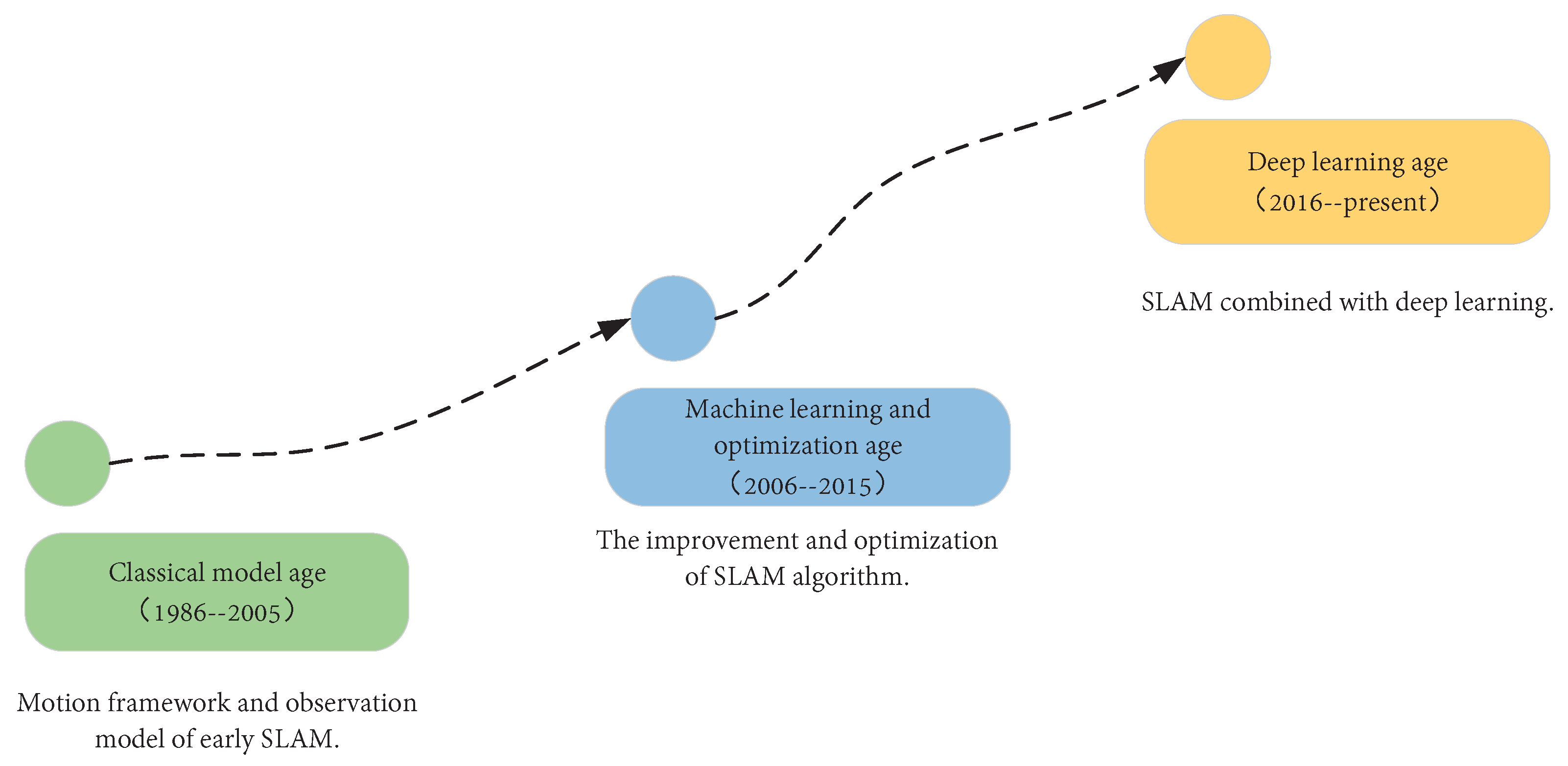
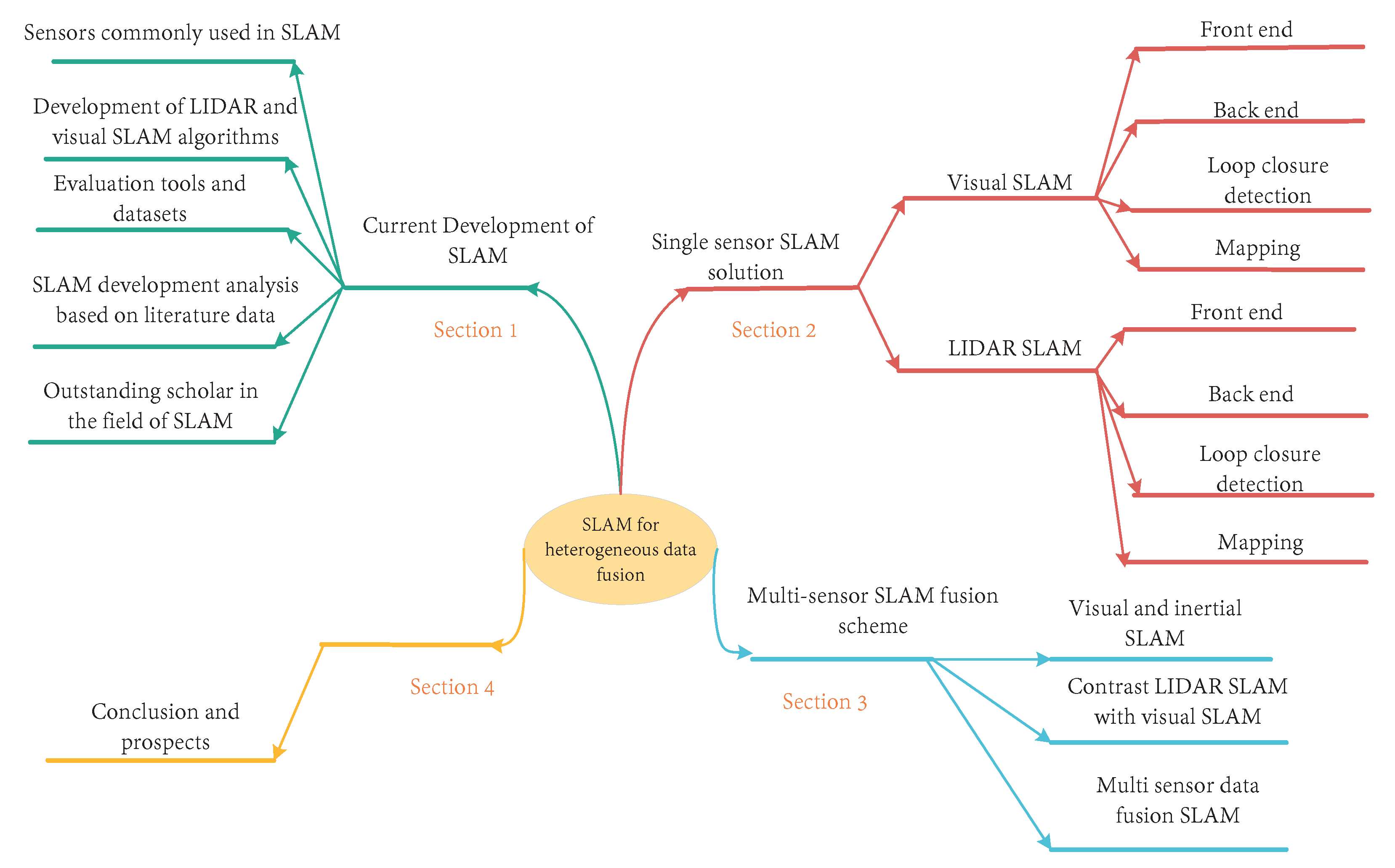
5. Conclusions and Prospect

After years of development, many excellent visual- and LIDAR-based SLAM algorithms have emerged, which have also been widely used in actual scenarios, such as indoor and outdoor mobile robots, AR, VR, and other virtual scenarios. Additionally, these algorithms show broad prospects for the development of SLAM technology. The traditional visual SLAM and LIDAR SLAM have their respective advantages and limitations: for example, their advantages include the range of scenarios they can be applied to, the precision of the localization and map building, the types of sensors, and the cost, but the algorithms encounter difficulty in complex scenes and are unable to meet the demands of robot autonomous navigation and human–computer interaction. As the performance of hardware and software in machine learning is constantly improving, computer LIDAR–visual–IMU fusion algorithms as well as various other sensor fusion algorithms, are being implemented. The fusion algorithms proposed thus far have made full use of the advantages of different sensors. Based on the characteristics of uncertainty and the traditional framework, researchers have conducted a large number of studies and fruitful results have been obtained, achieving superior performance in terms of building high-precision maps and eliminating cumulative errors that cannot be achieved only using a single sensor. In recent years, with the rise of the deep learning field, deep learning has shown its great potential in terms of image recognition and voice processing and received extensive attention from SLAM researchers. Therefore, multi-sensor fusion algorithms based on deep learning have been proposed, which, through training, can gather a large number of datasets. The deep learning method can obtain more abundant map information, and the whole system also has a stronger generalization ability.

The fusion system of SLAM and multiple sensors has achieved superior results in terms of robustness, accuracy, and advanced perception and has also attracted the attention of an increasing number of researchers. Multi-sensor fusion SLAM will fundamentally eliminate the limitations of different sensors themselves to improve the autonomous interaction ability of robots [222]. Combined with these studies, this paper puts forward the following prospects for the future of multi-sensor fusion SLAM:

(1) Development history and engineering applications. In recent years, although the fusion of multiple sensors in SLAM has resulted in some outstanding achievements, compared with the traditional pure visual and LIDAR SLAM, it is still in a stage of development. Furthermore, the participation of more sensors means that a vaster computing power and a more superior system are needed to eliminate useless information, which can seriously interfere with the real-time performance of SLAM. This situation will improve in the future with the continuous development of algorithms and the continuous updating of software and hardware. However, at the same time, we also want to improve its convenience, e.g., by making it easy to adjust and facilitate its maintenance.

(2) Theoretical support. Fusion methods based on uncertainty and traditional features are not used throughout the whole SLAM process, and most of the fusion methods are aimed at one of the four modules: front-end, back-end, loop closure detection, and mapping. Therefore, understanding how to apply the fusion method to the whole SLAM process is still a great challenge. At the same time, the features extracted by deep learning technology lack intuitive significance and a theoretical basis, and we cannot know what standard the computer uses to extract features. At present, the field of multi-sensor fusion based on RNNs is still a blank slate, and the traditional method still has great advantages.

(3) Human–computer interaction ability. Multiple sensors offer richer environmental information. In an actual scene, where the redundant information screened by the system is different from the information that needs to be obtained, it is still a difficult task to apply rich information to the autonomous interaction process of robots.

References

1. Shaohua, G.; Kailun, Y.; Hao, S.; Kaiwei, W. Bai, J. Review on Panoramic Imaging and Its Applications in Scene Understanding. IEEE Trans. Instrum. Meas. 2022, 71, 1–34. [Google Scholar]
2. Smith, R.C.; Cheeseman, P. On the Representation and Estimation of Spatial Uncertainty. Int. J. Robot. Res. 1986, 5, 56–68. [Google Scholar] [CrossRef]
3. Bresson, G.; Alsayed, Z.; Yu, L.; Glaser, S. Simultaneous Localization and Mapping: A Survey of Current Trends in Autonomous Driving. IEEE Trans. Intell. Veh. 2017, 2, 194–220. [Google Scholar] [CrossRef] [Green Version]
4. Durrant-Whyte, H.F. Uncertain geometry in robotics. IEEE J. Robot. Autom. 1988, 4, 23–31. [Google Scholar] [CrossRef]
5. Ayache, N.; Faugeras, O.D. Building, Registrating, and Fusing Noisy Visual Map. Int. J. Robot. Res. 1988, 7, 45–65. [Google Scholar] [CrossRef] [Green Version]
6. Crowley, J.L. World modeling and position estimation for a mobile robot using ultrasonic ranging. In Proceedings of the International Conference on Robotics and Automation, Scottsdale, AZ, USA, 14–19 May 1989; Volume 2, pp. 674–680. [Google Scholar] [CrossRef]
7. Chatila, R.; Laumond, J.-P. Position referencing and consistent world modeling for mobile robots. In Proceedings of the IEEE International Conference on Robotics and Automation, St. Louis, MO, USA, 25–28 March 1985; Volume 2, pp. 138–145. [Google Scholar]
8. Smith, R.C.; Self, M.; Cheeseman, P.C. Estimating Uncertain Spatial Relationships in Robotics. In Proceedings of the IEEE International Conference on Robotics and Automation, Raleigh, NC, USA, 31 March–3 April 1987; p. 850. [Google Scholar] [CrossRef]
9. Dissanayake, G.; Newman, P.; Clark, S.; Durrant-Whyte, H.F.; Csorba, M. A solution to the simultaneous localization and map building (SLAM) problem. IEEE Trans. Robotics Autom. 2001, 17, 229–241. [Google Scholar] [CrossRef] [Green Version]
10. Durrant-Whyte, H.F.; Rye, D.C.; Nebot, E.M. Localization of Autonomous Guided Vehicles; Robotics Research; Springer: London, UK, 1996; pp. 613–625. [Google Scholar] [CrossRef]
11. Leonard, J.J.; Feder, H.J.S. A Computationally Efficient Method for Large-Scale Concurrent Mapping and Localization; Robotics Research; Springer: London, UK, 2000; pp. 169–176. [Google Scholar] [CrossRef]
12. Castellanos, J.A.; Tardós, J.D.; Schmidt, G.K. Building a global map of the environment of a mobile robot: The importance of correlations. In Proceedings of the International Conference on Robotics and Automation, Albuquerque, NM, USA, 25 April 1997; Volume 1052, pp. 1053–1059. [Google Scholar]
13. Castellanos, J.A.; Martínez, J.M.; Neira, J.; Tardós, J.D. Experiments in Multisensor Mobile Robot Localization and Map Building. IFAC Proc. Vol. 1998, 31, 369–374. [Google Scholar] [CrossRef]
14. Guivant, J.E.; Nebot, E.M.; Baiker, S. Localization and map building using laser range sensors in outdoor applications. Field Robot. 2000, 17, 565–583. [Google Scholar] [CrossRef]
15. Williams, S.B.; Newman, P.; Dissanayake, G.; Durrant-Whyte, H.F. Autonomous underwater simultaneous localisation and map building. In Proceedings of the Proceedings 2000 ICRA. Millennium Conference. IEEE International Conference on Robotics and Automation. Symposia Proceedings (Cat. No.00CH37065), San Francisco, CA, USA, 24–28 April 2000; Volume 1792, pp. 1793–1798. [Google Scholar]
16. Chong, K.S.; Kleeman, L. Feature-Based Mapping in Real, Large Scale Environments Using an Ultrasonic Array. Int. J. Robot. Res. 1999, 18, 3–19. [Google Scholar]
17. Deans, M.C.; Hebert, M. Experimental Comparison of Techniques for Localization and Mapping Using a Bearing-Only Sensor; Experimental Robotics VII. Lecture Notes in Control and Information Sciences; Springer: Berlin/Heidelberg, Germany, 2000; Volume 271, pp. 395–404. [Google Scholar] [CrossRef]
18. Csorba, M. Simultaneous Localisation and Map Building; Springer Tracts in Advanced Robotics; Springer: Berlin/Heidelberg, Germany, 1997; Volume 23. [Google Scholar] [CrossRef] [Green Version]
19. Csorba, M.; Durrant-Whyte, H.F. New Approach to Map Building Using Relative Position Estimates. In Proceedings of SPIE AeroSense ’97, Orlando, FL, USA, 26 June 1997; Volume 3087, pp. 115–125. [Google Scholar]
20. Guivant, J.E.; Nebot, E.M. Optimization of the simultaneous localization and map-building algorithm for real-time implementation. IEEE Trans. Robot. Autom. 2001, 17, 242–257. [Google Scholar] [CrossRef] [Green Version]
21. Neira, J.; Tardós, J.D. Data association in stochastic mapping using the joint compatibility test. IEEE Trans. Robot. Autom. 2001, 17, 890–897. [Google Scholar] [CrossRef] [Green Version]
22. Julier, S.J.; Uhlmann, J.K. A counter example to the theory of simultaneous localization and map building. In Proceedings of the Proceedings 2001 ICRA. IEEE International Conference on Robotics and Automation (Cat. No.01CH37164), Seoul, Korea, 21–26 May 2001; Volume 4234, pp. 4238–4243. [Google Scholar]
23. Montemerlo, M.; Thrun, S.; Koller, D.; Wegbreit, B. FastSLAM: A Factored Solution to the Simultaneous Localization and Mapping Problem; AAAI, Artificial Intelligence: Edmonton, AB, Canada, 2002; Volume 50, pp. 240–248. [Google Scholar]
24. Sujan, V.A.; Dubowsky, S. Efficient Information-based Visual Robotic Mapping in Unstructured Environments. Int. J. Robot. Res. 2005, 24, 275–293. [Google Scholar] [CrossRef]
25. Lu, F.; Milios, E.E. Globally Consistent Range Scan Alignment for Environment Mapping. Auton. Robot. 1997, 4, 333–349. [Google Scholar] [CrossRef]
26. Gutmann, J.; Konolige, K. Incremental Mapping of Large Cyclic Environments. In Proceedings of the 1999 IEEE International Symposium on Computational Intelligence in Robotics and Automation. CIRA’99 (Cat. No.99EX375), Monterey, CA, USA, 8–9 November 1999; pp. 318–325. [Google Scholar] [CrossRef] [Green Version]
27. Folkesson, J.; Christensen, H.I. Graphical SLAM for Outdoor Applications. J. Field Robot. 2007, 24, 51–70. [Google Scholar] [CrossRef]
28. Grisetti, G.; Grzonka, S.; Stachniss, C.; Pfaff, P.; Burgard, W. Efficient estimation of accurate maximum likelihood maps in 3D. In Proceedings of the IEEE/RSJ International Conference on Intelligent Robots and System, San Diego, CA, USA, 29 October–2 November 2007; pp. 3472–3478. [Google Scholar]
29. Kschischang, F.R.; Frey, B.J.; Loeliger, H.-A. Factor graphs and the sum-product algorithm. IEEE Trans. Inf. Theory 2001, 47, 498–519. [Google Scholar] [CrossRef]
30. Durrant-Whyte, H.; Bailey, T. Simultaneous localization and mapping: Part I. IEEE Robot. Autom. Mag. 2006, 13, 99–110. [Google Scholar] [CrossRef] [Green Version]
31. Aulinas, J.; Petillot, Y.R.; Salvi, J.; Lladó, X. The SLAM Problem: A Survey. In Proceedings of the 11th International Conference of the Catalan Association for Artificial Intelligence, Amsterdam, The Netherlands, 3 July 2008; pp. 363–371. [Google Scholar]
32. Grisetti, G.; Kümmerle, R.; Stachniss, C.; Burgard, W. A Tutorial on Graph-Based SLAM. IEEE Intell. Transp. Syst. Mag. 2010, 2, 31–43. [Google Scholar] [CrossRef]
33. Dissanayake, G.; Huang, S.; Wang, Z.; Ranasinghe, R. A review of recent developments in Simultaneous Localization and Mapping. In Proceedings of the International Conference on Industrial and Information Systems, Kandy, Sri Lanka, 16–19 August 2011; pp. 477–482. [Google Scholar]
34. Fraundorfer, F.; Scaramuzza, D. Visual Odometry: Part II: Matching, Robustness, Optimization, and Applications. IEEE Robot. Autom. Mag. 2012, 19, 78–90. [Google Scholar] [CrossRef] [Green Version]
35. Mur-Artal, R.; Montiel, J.M.M.; Tardós, J.D. ORB-SLAM: A Versatile and Accurate Monocular SLAM System. IEEE Trans. Robot. 2015, 31, 1147–1163. [Google Scholar] [CrossRef] [Green Version]
36. Li, R.; Wang, S.; Gu, D. DeepSLAM: A Robust Monocular SLAM System With Unsupervised Deep Learning. IEEE Trans. Ind. Electron. 2021, 68, 3577–3587. [Google Scholar] [CrossRef]
37. Bescos, B.; Fácil, J.M.; Civera, J.; Neira, J. DynaSLAM: Tracking, Mapping, and Inpainting in Dynamic Scenes. IEEE Robot. Autom. Lett. 2018, 3, 4076–4083. [Google Scholar] [CrossRef] [Green Version]
38. Han, X.F.; Laga, H.; Bennamoun, M. Image-Based 3D Object Reconstruction: State-of-the-Art and Trends in the Deep Learning Era. IEEE Trans. Pattern Anal. Mach. Intell. 2021, 43, 1578–1604. [Google Scholar] [CrossRef] [PubMed] [Green Version]
39. Li, C.; Wang, S.; Zhuang, Y.; Yan, F. Deep Sensor Fusion Between 2D Laser Scanner and IMU for Mobile Robot Localization. IEEE Sens. J. 2021, 21, 8501–8509. [Google Scholar] [CrossRef]
40. Cattaneo, D.; Vaghi, M.; Valada, A. LCDNet: Deep Loop Closure Detection and Point Cloud Registration for LiDAR SLAM. IEEE Trans. Robot. 2022, 38, 2074–2093. [Google Scholar] [CrossRef]
41. Huang, S.; Dissanayake, G. A critique of current developments in simultaneous localization and mapping. Int. J. Adv. Robot. Syst. 2016, 13, 1729881416669482. [Google Scholar] [CrossRef]
42. Mur-Artal, R.; Tardós, J.D. ORB-SLAM2: An Open-Source SLAM System for Monocular, Stereo, and RGB-D Cameras. IEEE Trans. Robot. 2017, 33, 1255–1262. [Google Scholar] [CrossRef] [Green Version]
43. Campos, C.; Elvira, R.; Rodríguez, J.J.G.; Montiel, J.M.M.; Tardós, J.D. ORB-SLAM3: An Accurate Open-Source Library for Visual, Visual–Inertial, and Multimap SLAM. IEEE Trans. Robot. 2021, 37, 1874–1890. [Google Scholar] [CrossRef]
44. Engel, J.; Koltun, V. Cremers, Direct Sparse Odometry. IEEE Trans. Pattern Anal. Mach. Intell. 2018, 40, 611–625. [Google Scholar] [CrossRef] [PubMed]
45. Forster, C.; Pizzoli, M.; Scaramuzza, D. SVO: Fast Semi-Direct Monocular Visual Odometry. In Proceedings of the 2014 IEEE International Conference on Robotics and Automation (ICRA), Hong Kong, China, 31 May–5 June 2014; pp. 15–22. [Google Scholar] [CrossRef] [Green Version]
46. Engel, J.J.; Schöps, T.; Cremers, D. LSD-SLAM: Large-Scale Direct Monocular SLAM; ECCV 2014. Lecture Notes in Computer Science; Springer: Cham, Switzerland, 2014; Volume 8690, pp. 834–849. [Google Scholar] [CrossRef] [Green Version]
47. Debeunne, C.; Vivet, D. A Review of Visual-LiDAR Fusion based Simultaneous Localization and Mapping. Sensors 2020, 20, 2068. [Google Scholar] [CrossRef] [PubMed] [Green Version]
48. Xu, X.B.; Zhang, L.; Yang, J.; Cao, C.F.; Wang, W.; Ran, Y.Y.; Tan, Z.Y.; Luo, M.Z. A Review of Multi-Sensor Fusion SLAM Systems Based on 3D LIDAR. Remote Sens. 2022, 14, 27. [Google Scholar] [CrossRef]
49. de Medeiros Esper, I.; Smolkin, O.; Manko, M.; Popov, A.; From, P.J.; Mason, A. Evaluation of RGB-D Multi-Camera Pose Estimation for 3D Reconstruction. Appl. Sci. 2022, 12, 4134. [Google Scholar] [CrossRef]
50. Available online: https://alex007.blog.csdn.net/article/details/120389614 (accessed on 4 October 2022).
51. Available online: https://www.bilibili.com/video/BV1Lf4y1s7Qa/?vd_source=e427cefaf96e6ad70c9e5d73f26b3d1e (accessed on 4 October 2022).
52. Davison, A.J.; Reid, I.D.; Molton, N.D.; Stasse, O. MonoSLAM: Real-Time Single Camera SLAM. IEEE Trans. Pattern Anal. Mach. Intell. 2007, 29, 1052–1067. [Google Scholar] [CrossRef] [Green Version]
53. Klein, G.; Murray, D. Parallel Tracking and Mapping for Small AR Workspaces. In Proceedings of the 2007 6th IEEE and ACM International Symposium on Mixed and Augmented Reality, Washington, DC, USA, 13–16 November 2007; pp. 225–234. [Google Scholar] [CrossRef]
54. Forster, C.; Zhang, Z.; Gassner, M.; Werlberger, M.; Scaramuzza, D. SVO: Semidirect Visual Odometry for Monocular and Multicamera Systems. IEEE Trans. Robot. 2017, 33, 249–265. [Google Scholar] [CrossRef] [Green Version]
55. Newcombe, R.A.; Lovegrove, S.J.; Davison, A.J. DTAM: Dense Tracking and Mapping in Real-Time. In Proceedings of the International Conference on Computer Vision, Barcelona, Spain, 6–13 November 2011; pp. 2320–2327. [Google Scholar] [CrossRef] [Green Version]
56. Kerl, C.; Sturm, J.; Cremers, D. Dense Visual SLAM for RGB-D Cameras. In Proceedings of the 2013 IEEE/RSJ International Conference on Intelligent Robots and Systems, Tokyo, Japan, 3–7 November 2013; pp. 2100–2106. [Google Scholar] [CrossRef] [Green Version]
57. Labbé, M.; Michaud, F. RTAB-Map as an open-source lidar and visual simultaneous localization and mapping library for large-scale and long-term online operation. J. Field Robot. 2019, 36, 416–446. [Google Scholar] [CrossRef]
58. Endres, F.; Hess, J.; Sturm, J.; Cremers, D.; Burgard, W. 3-D Mapping With an RGB-D Camera. IEEE Trans. Robot. 2014, 30, 177–187. [Google Scholar] [CrossRef]
59. Whelan, T.; Salas-Moreno, R.F.; Glocker, B.; Davison, A.J.; Leutenegger, S. ElasticFusion: Real-time dense SLAM and light source estimation. Int. J. Robot. Res. 2016, 35, 1697–1716. [Google Scholar] [CrossRef] [Green Version]
60. Grisetti, G.; Stachniss, C.; Burgard, W. Improved Techniques for Grid Mapping With Rao-Blackwellized Particle Filters. IEEE Trans. Robot. 2007, 23, 34–46. [Google Scholar] [CrossRef] [Green Version]
61. Kohlbrecher, S.; Stryk, O.; Meyer, J.; Klingauf, U. A Flexible and Scalable SLAM System with Full 3D Motion Estimation. In Proceedings of the 2011 IEEE International Symposium on Safety, Security, and Rescue Robotics, Kyoto, Japan, 1–5 November 2011; pp. 155–160. [Google Scholar] [CrossRef] [Green Version]
62. Hess, W.; Kohler, D.; Rapp, H.; Andor, D. Real-Time Loop Closure in 2D LIDAR SLAM. In Proceedings of the 2016 IEEE International Conference on Robotics and Automation (ICRA), Stockholm, Sweden, 16–21 May 2016; pp. 1271–1278. [Google Scholar] [CrossRef]
63. Zhang, J.; Singh, S. LOAM: Lidar Odometry and Mapping in real-time. In Proceedings of the Robotics: Science and Systems Conference (RSS), Computer Science, Berkeley, CA, USA, 12–16 July 2014; pp. 109–111. [Google Scholar]
64. Zhang, J.; Singh, S. Visual-Lidar Odometry and Mapping: Low-Drift, Robust, and Fast. In Proceedings of the 2015 IEEE International Conference on Robotics and Automation (ICRA), Seattle, WA, USA, 25–30 May 2015; pp. 2174–2181. [Google Scholar] [CrossRef]
65. Zhang, J.; Singh, S. Laser-visual-inertial Odometry and Mapping with High Robustness and Low Drift. J. Field Robot. 2018, 35, 1242–1264. [Google Scholar] [CrossRef]
66. Shan, T.; Englot, B. LeGO-LOAM: Lightweight and Ground-Optimized Lidar Odometry and Mapping on Variable Terrain. In Proceedings of the 2018 IEEE/RSJ International Conference on Intelligent Robots and Systems (IROS), Madrid, Spain, 1–5 October 2018; pp. 4758–4765. [Google Scholar] [CrossRef]
67. Ye, H.; Chen, Y.; Liu, M. Tightly Coupled 3D Lidar Inertial Odometry and Mapping. In Proceedings of the 2019 International Conference on Robotics and Automation (ICRA), Montreal, QC, Canada, 20–24 May 2019; pp. 3144–3150. [Google Scholar] [CrossRef] [Green Version]
68. Shan, T.; Englot, B.; Meyers, D.; Wang, W.; Ratti, C.; Rus, D. LIO-SAM: Tightly-Coupled Lidar Inertial Odometry via Smoothing and Mapping. In Proceedings of the 2020 IEEE/RSJ International Conference on Intelligent Robots and Systems (IROS), Las Vegas, NV, USA, 25–19 October 2020; pp. 5135–5142. [Google Scholar]
69. EVO. Available online: https://github.com/MichaelGrupp/evo (accessed on 21 September 2022).
70. Bodin, B.; Wagstaff, H.; Saecdi, S.; Nardi, L.; Vespa, E.; Mawer, J.; Nisbet, A.; Luján, M.; Furber, S.; Davison, A.J.; et al. SLAMBench2: Multi-Objective Head-to-Head Benchmarking for Visual SLAM. In Proceedings of the 2018 IEEE International Conference on Robotics and Automation (ICRA), Brisbane, Australia, 21–25 May 2018; pp. 3637–3644. [Google Scholar]
71. Leutenegger, S.; Lynen, S.; Bosse, M.; Siegwart, R.; Furgale, P. Keyframe-based visual–inertial odometry using nonlinear optimization. Int. J. Robot. Res. 2014, 34, 314–334. [Google Scholar] [CrossRef] [Green Version]
72. TUM RGB-D. Available online: https://vision.in.tum.de/data/datasets/rgbd-dataset (accessed on 21 September 2022).
73. TUM MonoVo. Available online: http://vision.in.tum.de/mono-dataset (accessed on 21 September 2022).
74. TUM VI. Available online: https://vision.in.tum.de/data/datasets/visual-inertial-dataset (accessed on 21 September 2022).
75. KITTI. Available online: http://www.cvlibs.net/datasets/kitti/ (accessed on 21 September 2022).
76. Oxford. Available online: http://robotcar-dataset.robots.ox.ac.uk/datasets/ (accessed on 21 September 2022).
77. ASL Kinect. Available online: http://projects.asl.ethz.ch/datasets/doku.php (accessed on 21 September 2022).
78. EuRoc. Available online: http://projects.asl.ethz.ch/datasets/doku.php?id=kmavvisualinertialdatasets#downloads (accessed on 21 September 2022).
79. ICL-NUIM. Available online: http://www.doc.ic.ac.uk/~ahanda/VaFRIC/iclnuim.html (accessed on 21 September 2022).
80. VaFRIC. Available online: http://www.doc.ic.ac.uk/~ahanda/VaFRIC/index.html (accessed on 21 September 2022).
81. EuRoC. Available online: http://projects.asl.ethz.ch/datasets/doku.php?id=kmavvisualinertialdatasets (accessed on 21 September 2022).
82. Gupta, A.; Fernando, X. Simultaneous Localization and Mapping (SLAM) and Data Fusion in Unmanned Aerial Vehicles: Recent Advances and Challenges. Drones 2022, 6, 85. [Google Scholar] [CrossRef]
83. Cadena, C.; Carlone, L.; Carrillo, H.; Latif, Y.; Scaramuzza, D.; Neira, J.; Reid, I.; Leonard, J.J. Past, Present, and Future of Simultaneous Localization and Mapping: Toward the Robust-Perception Age. IEEE Trans. Robot. 2016, 32, 1309–1332. [Google Scholar] [CrossRef] [Green Version]
84. Taheri, H.; Xia, Z.C. SLAM, definition and evolution. Eng. Appl. Artif. Intell. 2021, 97, 104032. [Google Scholar] [CrossRef]
85. Scaramuzza, D.; Fraundorfer, F. Visual Odometry: Part I: The First 30 Years and Fundamentals. IEEE Robot. Autom. Mag. 2011, 18, 80–92. [Google Scholar] [CrossRef]
86. Azzam, R.; Taha, T.; Huang, S.; Zweiri, Y. Feature-based visual simultaneous localization and mapping: A survey. SN Appl. Sci. 2020, 2, 224. [Google Scholar] [CrossRef] [Green Version]
87. Harris, C.; Stephens, M. A combined corner and edge detector. Alvey Vis. Conf. 1988, 15, 147–151. [Google Scholar]
88. Rosten, E.; Drummond, T. Machine Learning for High-Speed Corner Detection; Springer: Berlin/Heidelberg, Germany, 2006; pp. 430–443. [Google Scholar]
89. Shi, J.; Thomasi, C. Good Features to Track. In Proceedings of the 1994 IEEE Conference on Computer Vision and Pattern Recognition, Columbus, OH, USA, 23–28 June 1994; pp. 593–600. [Google Scholar] [CrossRef]
90. Lowe, D.G. Distinctive Image Features from Scale-Invariant Keypoints. Int. J. Comput. Vis. 2004, 60, 91–110. [Google Scholar] [CrossRef]
91. Bay, H.; Ess, A.; Tuytelaars, T.; Van Gool, L. Speeded-Up Robust Features (SURF). Comput. Vis. Image Underst. 2008, 110, 346–359. [Google Scholar] [CrossRef]
92. Rublee, E.; Rabaud, V.; Konolige, K.; Bradski, G.R. ORB: An efficient alternative to SIFT or SURF. In Proceedings of the 2011 International Conference on Computer Vision, Barcelona, Spain, 6–13 November 2011; pp. 2564–2571. [Google Scholar]
93. Muja, M.; Lowe, D.G. Fast Approximate Nearest Neighbors with Automatic Algorithm Configuration. In Proceedings of the Fourth International Conference on Computer Vision Theory and Applications, Lisboa, Portugal, 5–8 February 2009; pp. 331–340. [Google Scholar]
94. Rusinkiewicz, S.; Levoy, M. Efficient Variants of the ICP Algorithm. In Proceedings of the Third International Conference on 3-D Digital Imaging and Modeling, Quebec City, QC, Canada, 28 May–1 June 2001; pp. 145–152. [Google Scholar]
95. Lepetit, V.; Moreno-Noguer, F.; Fua, P. EPnP: An Accurate O(n) Solution to the PnP Problem. Int. J. Comput. Vis. 2008, 81, 155. [Google Scholar] [CrossRef] [Green Version]
96. Zhu, K.; Jiang, X.; Fang, Z.; Gao, Y.; Fujita, H.; Hwang, J.-N. Photometric transfer for direct visual odometry. Knowl.Based Syst. 2021, 213, 106671. [Google Scholar] [CrossRef]
97. Janabi-Sharifi, F.; Marey, M. A Kalman-Filter-Based Method for Pose Estimation in Visual Servoing. IEEE Trans. Robot. 2010, 26, 939–947. [Google Scholar] [CrossRef]
98. Li, S.; Ni, P. Square-Root Unscented Kalman Filter Based Simultaneous Localization and Mapping. In Proceedings of the 2010 IEEE International Conference on Information and Automation, Harbin, China, 20–23 June 2010; pp. 2384–2388. [Google Scholar] [CrossRef]
99. Sim, R.; Elinas, P.; Little, J.J. A Study of the Rao-Blackwellised Particle Filter for Efficient and Accurate Vision-Based SLAM. Int. J. Comput. Vis. 2007, 74, 303–318. [Google Scholar] [CrossRef] [Green Version]
100. Lee, J.S.; Nam, S.Y.; Chung, W.K. Robust RBPF-SLAM for Indoor Mobile Robots Using Sonar Sensors in Non-Static Environments. Adv. Robot. 2011, 25, 1227–1248. [Google Scholar] [CrossRef]
101. Gil, A.; Reinoso, Ó.; Ballesta, M.; Juliá, M. Multi-robot visual SLAM using a Rao-Blackwellized particle filter. Robot. Auton. Syst. 2010, 58, 68–80. [Google Scholar] [CrossRef]
102. Sibley, G.; Matthies, L.; Sukhatme, G. Sliding Window Filter with Application to Planetary Landing. J. Field Robot. 2010, 27, 587–608. [Google Scholar] [CrossRef]
103. Paz, L.M.; TardÓs, J.D.; Neira, J. Divide and Conquer: EKF SLAM in O(n). IEEE Trans. Robot. 2008, 24, 1107–1120. [Google Scholar] [CrossRef]
104. Grasa, O.G.; Civera, J.; Montiel, J.M.M. EKF Monocular SLAM with Relocalization for Laparoscopic Sequences. In 2011 IEEE International Conference on Robotics and Automation; IEEE: Piscataway Township, NJ, USA, 2011; pp. 4816–4821. [Google Scholar] [CrossRef]
105. Lourakis, M.I.A.; Argyros, A.A. SBA: A software package for generic sparse bundle adjustment. ACM Trans. Math. Softw. (TOMS) 2009, 36, 1–30. [Google Scholar] [CrossRef]
106. Horn, B.K.P. Closed-form solution of absolute orientation using unit quaternions. J. Opt. Soc. Am. A-Opt. Image Sci. Vis. 1987, 4, 629–642. [Google Scholar] [CrossRef]
107. Ulrich, I.; Nourbakhsh, I. Appearance-Based Place Recognition for Topological Localization. In Proceedings of the 2000 ICRA. Millennium Conference. IEEE International Conference on Robotics and Automation. Symposia Proceedings (Cat. No.00CH37065), San Francisco, CA, USA, 24–28 April 2000; Volume 1022, pp. 1023–1029. [Google Scholar]
108. Jogan, M.; Leonardis, A. Robust Localization Using Panoramic View-Based Recognition. In Proceedings of the 15th International Conference on Pattern Recognition. ICPR-2000, Barcelona, Spain, 3–7 September 2000; Volume 134, pp. 136–139. [Google Scholar]
109. Mikolajczyk, K.; Tuytelaars, T.; Schmid, C.; Zisserman, A.; Matas, J.; Schaffalitzky, F.; Kadir, T.; Gool, L.V. A Comparison of Affine Region Detectors. Int. J. Comput. Vis. 2005, 65, 43–72. [Google Scholar] [CrossRef] [Green Version]
110. Newman, P.; Cole, D.; Ho, K. Outdoor SLAM Using Visual Appearance and Laser Ranging. In Proceedings of the 2006 IEEE International Conference on Robotics and Automation ICRA, Orlando, FL, USA, 15–19 May; 2006; pp. 1180–1187. [Google Scholar]
111. Cummins, M.; Newman, P. FAB-MAP: Probabilistic Localization and Mapping in the Space of Appearance. Int. J. Robot. Res. 2008, 27, 647–665. [Google Scholar] [CrossRef]
112. Fraundorfer, F.; Wu, C.; Frahm, J.-M.; Pollefeys, M. Visual Word Based Location Recognition in 3D Models Using Distance Augmented Weighting. In Proceedings of the International Symposium on 3D Data Processing, Visualization and Transmission Georgia Institute of Technology, Paris, France, 17–20 May 2008; pp. 331–340. [Google Scholar]
113. Zhao, J.; Li, T.; Yang, T.; Zhao, L.; Huang, S. 2D Laser SLAM With Closed Shape Features: Fourier Series Parameterization and Submap Joining. IEEE Robot. Autom. Lett. 2021, 6, 1527–1534. [Google Scholar] [CrossRef]
114. Besl, P.J.; Mckay, H.D. A method for registration of 3-D shapes. IEEE Trans. Pattern Anal. Mach. Intell. 1992, 14, 239–256. [Google Scholar] [CrossRef] [Green Version]
115. Censi, A. An ICP Variant Using a Point-to-Line Metric. In Proceedings of the 2008 IEEE International Conference on Robotics and Automation, Pasadena, CA, USA, 19–23 May 2008; pp. 19–25. [Google Scholar] [CrossRef] [Green Version]
116. Diosi, A.; Kleeman, L. Fast Laser Scan Matching using Polar Coordinates. Int. J. Robot. Res. 2007, 26, 1125–1153. [Google Scholar] [CrossRef]
117. Konolige, K.; Grisetti, G.; Kümmerle, R.; Burgard, W.; Limketkai, B.; Vincent, R. Efficient Sparse Pose Adjustment for 2D mapping. In Proceedings of the 2010 IEEE/RSJ International Conference on Intelligent Robots and Systems, Taipei, Taiwan, 18–22 October 2010; pp. 22–29. [Google Scholar]
118. Monar, F.M.; Triebel, R.; Moreno, L.E.; Siegwart, R.Y. Two different tools for three-dimensional mapping: DE-based scan matching and feature-based loop detection. Robotica 2013, 32, 19–41. [Google Scholar]
119. Liu, Y.; Zhao, C.; Ren, M. An Enhanced Hybrid Visual–Inertial Odometry System for Indoor Mobile Robot. Sensors 2022, 22, 2930. [Google Scholar] [CrossRef]
120. Xie, H.; Chen, W.; Wang, J. Hierarchical forest based fast online loop closure for low-latency consistent visual-inertial SLAM. Robot. Auton. Syst. 2022, 151, 104035. [Google Scholar] [CrossRef]
121. Lee, W.; Eckenhoff, K.; Yang, Y.; Geneva, P.; Huang, G. Visual-Inertial-Wheel Odometry with Online Calibration. In Proceedings of the IROS, Las Vegas, NV, USA, 25–29 October 2020; pp. 4559–4566. [Google Scholar]
122. Cheng, J.; Zhang, L.; Chen, Q. An Improved Initialization Method for Monocular Visual-Inertial SLAM. Electronics 2021, 10, 3063. [Google Scholar] [CrossRef]
123. Jung, J.H.; Cha, J.; Chung, J.Y.; Kim, T.I.; Seo, M.H.; Park, S.Y.; Yeo, J.Y.; Park, C.G. Monocular Visual-Inertial-Wheel Odometry Using Low-Grade IMU in Urban Areas. IEEE Trans. Intell. Transp. Syst. 2022, 23, 925–938. [Google Scholar] [CrossRef]
124. Falquez, J.M.; Kasper, M.; Sibley, G. Inertial aided dense & semi-dense methods for robust direct visual odometry. In Proceedings of the 2016 IEEE/RSJ International Conference on Intelligent Robots and Systems (IROS), Daejeon, Korea, 9–14 October 2016; pp. 3601–3607. [Google Scholar]
125. Mourikis, A.I.; Roumeliotis, S.I. A Multi-State Constraint Kalman Filter for Vision-aided Inertial Navigation. In Proceedings of the 2007 IEEE International Conference on Robotics and Automation, Rome, Italy, 10–14 April 2007; pp. 3565–3572. [Google Scholar] [CrossRef]
126. Bloesch, M.; Omari, S.; Hutter, M.; Siegwart, R.Y. Robust visual inertial odometry using a direct EKF-based approach. In Proceedings of the 2015 IEEE/RSJ International Conference on Intelligent Robots and Systems (IROS), Hamburg, Germany, 28 September–2 October 2015; pp. 298–304. [Google Scholar]
127. Qin, T.; Li, P.; Shen, S. VINS-Mono: A Robust and Versatile Monocular Visual-Inertial State Estimator. IEEE Trans. Robot. 2018, 34, 1004–1020. [Google Scholar] [CrossRef] [Green Version]
128. Malartre, F.; Feraud, T.; Debain, C.; Chapuis, R. Digital Elevation Map Estimation by Vision-Lidar Fusion. In Proceedings of the 2009 IEEE International Conference on Robotics and Biomimetics (ROBIO), Guilin, China, 19–23 December 2009; pp. 523–528. [Google Scholar] [CrossRef]
129. Fengchi, S.; Yuan, Z.; Chao, L.; Yalou, H. Research on Active SLAM with Fusion of Monocular Vision and Laser Range Data. In Proceedings of the 2010 8th World Congress on Intelligent Control and Automation, Jinan, China, 7–9 July 2010; pp. 6550–6554. [Google Scholar]
130. Iocchi, L.; Pellegrini, S.; Tipaldi, G.D. Building Multi-Level Planar Maps Integrating LRF, Stereo Vision and IMU Sensors. In Proceedings of the 2007 IEEE International Workshop on Safety, Security and Rescue Robotics, Rome, Italy, 27–29 September 2007; pp. 1–6. [Google Scholar]
131. Aycard, O.; Baig, Q.; Bota, S.; Nashashibi, F.; Nedevschi, S.; Pantilie, C.; Parent, M.; Resende, P.; Vu, T.D. Intersection Safety Using Lidar and Stereo Vision Sensors. In Proceedings of the 2011 IEEE Intelligent Vehicles Symposium (IV), Baden-Baden, Germany, 5–9 June 2011; pp. 863–869. [Google Scholar]
132. Collier, J.; Se, S.; Kotamraju, V. Multi-Sensor Appearance-Based Place Recognition. In Proceedings of the 2013 International Conference on Computer and Robot Vision, Regina, SK, Canada, 28–31 May 2013; pp. 128–135. [Google Scholar]
133. Magree, D.; Johnson, E.N. Combined Laser and Vision-Aided Inertial Navigation for an Indoor Unmanned Aerial Vehicle. In Proceedings of the 2014 American Control Conference, Portland, OR, USA, 4–6 June 2014; pp. 1900–1905. [Google Scholar]
134. Wang, S.; Kobayashi, Y.; Ravankar, A.A.; Ravankar, A.; Emaru, T. A Novel Approach for Lidar-Based Robot Localization in a Scale-Drifted Map Constructed Using Monocular SLAM. Sensors 2019, 19, 2230. [Google Scholar] [CrossRef] [PubMed] [Green Version]
135. Huh, S.; Shim, D.H.; Kim, J. Integrated Navigation System Using Camera and Gimbaled Laser Scanner for Indoor and Outdoor Autonomous Flight of UAVs. In Proceedings of the 2013 IEEE/RSJ International Conference on Intelligent Robots and Systems, Tokyo, Japan, 3–7 November 2013; pp. 3158–3163. [Google Scholar]
136. Lopez, E.; Garcia, S.; Barea, R.; Bergasa, L.M.; Molinos, E.J.; Arroyo, R.; Romera, E.; Pardo, S. A Multi-Sensorial Simultaneous Localization and Mapping (SLAM) System for Low-Cost Micro Aerial Vehicles in GPS-Denied Environments. Sensors 2017, 17, 802. [Google Scholar] [CrossRef] [PubMed]
137. Bi, Y.; Qin, H.; Shan, M.; Li, J.; Liu, W.; Lan, M.; Chen, B.M. An Autonomous Quadrotor for Indoor Exploration with Laser Scanner and Depth Camera. In Proceedings of the 2016 12th IEEE International Conference on Control and Automation (ICCA), Kathmandu, Nepal, 1–3 June 2016; pp. 50–55. [Google Scholar]
138. De Silva, V.; Roche, J.; Kondoz, A. Robust Fusion of LiDAR and Wide-Angle Camera Data for Autonomous Mobile Robots. Sensors 2018, 18, 2730. [Google Scholar] [CrossRef]
139. Vasquez, B.P.E.A.; Gonzalez, R.; Matia, F.; Puente, P.D.L. Sensor Fusion for Tour-Guide Robot Localization. IEEE Access 2018, 6, 78947–78964. [Google Scholar] [CrossRef]
140. Andert, F.; Ammann, N.; Maass, B. Lidar-Aided Camera Feature Tracking and Visual SLAM for Spacecraft Low-Orbit Navigation and Planetary Landing; Springer International Publishing: Cham, Switzrland, 2015; pp. 605–623. [Google Scholar]
141. Seo, Y.; Chou, C.C. A Tight Coupling of Vision-Lidar Measurements for an Effective Odometry. In Proceedings of the 2019 IEEE Intelligent Vehicles Symposium (IV), Paris, France, 9–12 June 2019; pp. 1118–1123. [Google Scholar] [CrossRef]
142. Yin, L.; Luo, B.; Wang, W.; Yu, H.; Wang, C.; Li, C. CoMask: Corresponding Mask-Based End-to-End Extrinsic Calibration of the Camera and LiDAR. Remote Sens. 2020, 12, 1925. [Google Scholar] [CrossRef]
143. Zuo, X.; Geneva, P.; Yang, Y.; Ye, W.; Liu, Y.; Huang, G. Visual-Inertia Localization With Prior LiDAR Map Constraints. IEEE Robot. Autom. Lett. 2019, 4, 3394–3401. [Google Scholar] [CrossRef]
144. Pascoe, G.; Maddern, W.; Newman, P. Direct Visual Localisation and Calibration for Road Vehicles in Changing City Environments. In Proceedings of the 2015 IEEE International Conference on Computer Vision Workshop (ICCVW), Santiago, Chile, 7–13 December 2015; pp. 98–105. [Google Scholar]
145. Shin, M.; Kim, J.; Jeong, J.; Park, J.B. 3D LiDAR-Based Point Cloud Map Registration: Using Spatial Location of Visual Features. In Proceedings of the 2nd International Conference on Robotics and Automation Engineering (ICRAE), Santiago, Chile, 29–31 December 2017; pp. 373–378. [Google Scholar]
146. Chen, M.; Yang, S.; Yi, X.; Wu, D. Real-Time 3D Mapping Using a 2D Laser Scanner and IMU-Aided Visual SLAM. In Proceedings of the 2017 IEEE International Conference on Real-Time Computing and Robotics (RCAR), Okinawa, Japan, 14–18 July 2017; pp. 297–302. [Google Scholar]
147. Zhu, Z.; Yang, S.; Dai, H. Enhanced Visual Loop Closing for Laser-Based SLAM. In Proceedings of the 2018 IEEE 29th International Conference on Application-Specific Systems, Architectures and Processors (ASAP), Milan, Italy, 10–12 July 2018; pp. 1–4. [Google Scholar]
148. Huang, K.; Xiao, J.; Stachniss, C. Accurate Direct Visual-Laser Odometry with Explicit Occlusion Handling and Plane Detection. In Proceedings of the 2019 International Conference on Robotics and Automation (ICRA), Montreal, QC, Canada, 20–24 May 2019; pp. 1295–1301. [Google Scholar]
149. Zhou, G.; Yuan, H.; Zhu, S.; Huang, Z.; Fan, Y.; Zhong, X.; Du, R.; Gu, J. Visual Localization in a Prior 3D LiDAR Map Combining Points and Lines. In Proceedings of the 2021 IEEE International Conference on Robotics and Biomimetics (ROBIO), Sanya, China, 27–31 December 2021; pp. 1198–1203. [Google Scholar]
150. Qian, J.; Chen, K.; Chen, Q.; Yang, Y.; Zhang, J.; Chen, S. Robust Visual-Lidar Simultaneous Localization and Mapping System for UAV. IEEE Geosci. Remote. Sens. Lett. 2022, 19, 1–5. [Google Scholar] [CrossRef]
151. Wang, W.; Liu, J.; Wang, C.; Luo, B.; Zhang, C. DV-LOAM: Direct Visual LiDAR Odometry and Mapping. Remote. Sens. 2021, 13, 3340. [Google Scholar] [CrossRef]
152. Gawel, A.; Cieslewski, T.; Dubé, R.; Bosse, M.; Siegwart, R.; Nieto, J. Structure-Based Vision-Laser Matching. In Proceedings of the 2016 IEEE/RSJ International Conference on Intelligent Robots and Systems (IROS), Daejeon, Korea, 9–14 October 2016; pp. 182–188. [Google Scholar]
153. Mo, J.; Sattar, J. A Fast and Robust Place Recognition Approach for Stereo Visual Odometry Using LiDAR Descriptors. In Proceedings of the 2020 IEEE/RSJ International Conference on Intelligent Robots and Systems (IROS), Las Vegas, NV, USA, 25–29 October 2021; pp. 5893–5900. [Google Scholar]
154. Wu, Q.; Sun, K.; Zhang, W.; Huang, C.; Wu, X. Visual and LiDAR-Based for the Mobile 3D Mapping. In Proceedings of the 2016 IEEE International Conference on Robotics and Biomimetics (ROBIO), Qingdao, China, 3–7 December 2016; pp. 1522–1527. [Google Scholar]
155. Chavez-Garcia, R.O.; Aycard, O. Multiple Sensor Fusion and Classification for Moving Object Detection and Tracking. IEEE Trans. Intell. Transp. Syst. 2016, 17, 525–534. [Google Scholar] [CrossRef] [Green Version]
156. Chan, S.H.; Wu, P.T.; Fu, L.C. Robust 2D Indoor Localization Through Laser SLAM and Visual SLAM Fusion. In Proceedings of the 2018 IEEE International Conference on Systems, Man, and Cybernetics (SMC), Miyazaki, Japan, 7–10 October 2018; pp. 1263–1268. [Google Scholar]
157. Jin, Z.; Shao, Y.; So, M.; Sable, C.; Shlayan, N.; Luchtenburg, D.M. A Multisensor Data Fusion Approach for Simultaneous Localization and Mapping. In Proceedings of the 2019 IEEE Intelligent Transportation Systems Conference (ITSC), Auckland, New Zealand, 27–30 October 2019; pp. 1317–1322. [Google Scholar]
158. Tao, Y.; He, Y.; Ma, X.; Xu, H.; Hao, J.; Feng, J. SLAM Method Based on Multi-Sensor Information Fusion. In Proceedings of the 2021 International Conference on Computer Network, Electronic and Automation (ICCNEA), Xi’an, China, 24–26 September 2021; pp. 289–293. [Google Scholar] [CrossRef]
159. Giubilato, R.; Chiodini, S.; Pertile, M.; Debei, S. Scale Correct Monocular Visual Odometry Using a LiDAR Altimeter. In Proceedings of the 2018 IEEE/RSJ International Conference on Intelligent Robots and Systems (IROS), Madrid, Spain, 1–5 October 2018; pp. 3694–3700. [Google Scholar] [CrossRef]
160. Kim, Y.; Jeong, J.; Kim, A. Stereo Camera Localization in 3D LiDAR Maps. In Proceedings of the 2018 IEEE/RSJ International Conference on Intelligent Robots and Systems (IROS), Madrid, Spain, 1–5 October 2018; pp. 1–9. [Google Scholar]
161. Shin, Y.; Park, Y.S.; Kim, A. Direct Visual SLAM Using Sparse Depth for Camera-LiDAR System. In Proceedings of the 2018 IEEE International Conference on Robotics and Automation (ICRA), Brisbane, Australia, 21–25 May 2018; pp. 5144–5151. [Google Scholar]
162. Shin, Y.-S.; Park, Y.S.; Kim, A. DVL-SLAM: Sparse depth enhanced direct visual-LiDAR SLAM. Auton. Robot. 2020, 44, 115–130. [Google Scholar] [CrossRef]
163. Majdik, A.L.; Szoke, I.; Tamas, L.; Popa, M.; Lazea, G. Laser and Vision Based Map Building Techniques for Mobile Robot Navigation. In Proceedings of the 2010 IEEE International Conference on Automation, Quality and Testing, Robotics (AQTR), Cluj-Napoca, Romania, 28–30 May 2010; pp. 1–6. [Google Scholar]
164. Houben, S.; Droeschel, D.; Behnke, S. Joint 3D Laser and Visual Fiducial Marker Based SLAM for a Micro Aerial Vehicle. In Proceedings of the 2016 IEEE International Conference on Multisensor Fusion and Integration for Intelligent Systems (MFI), Baden-Baden, Germany, 19–21 September 2016; pp. 609–614. [Google Scholar]
165. Jiang, G.L.; Yin, L.; Jin, S.K.; Tian, C.R.; Ma, X.B.; Ou, Y.S. A Simultaneous Localization and Mapping (SLAM) Framework for 2.5D Map Building Based on Low-Cost LiDAR and Vision Fusion. Appl. Sci. 2019, 9, 2105. [Google Scholar] [CrossRef] [Green Version]
166. Mu, L.; Yao, P.; Zheng, Y.; Chen, K.; Wang, F.; Qi, N. Research on SLAM Algorithm of Mobile Robot Based on the Fusion of 2D LiDAR and Depth Camera. IEEE Access 2020, 8, 157628–157642. [Google Scholar] [CrossRef]
167. Chen, S.; Zhou, B.; Jiang, C.; Xue, W.; Li, Q. A LiDAR/Visual SLAM Backend with Loop Closure Detection and Graph Optimization. Remote. Sens. 2021, 13, 2720. [Google Scholar] [CrossRef]
168. Yan, M.; Wang, J.; Li, J.; Zhang, C. Loose Coupling Visual-Lidar Odometry by Combining VISO2 and LOAM. In Proceedings of the 2017 36th Chinese Control Conference (CCC), Dalian, China, 26–28 July 2017; pp. 6841–6846. [Google Scholar]
169. Camurri, M.; Ramezani, M.; Nobili, S.; Fallon, M. Pronto: A Multi-Sensor State Estimator for Legged Robots in Real-World Scenarios. Front. Robot. AI 2020, 7, 68. [Google Scholar] [CrossRef] [PubMed]
170. Alliez, P.; Bonardi, F.; Bouchafa, S.; Didier, J.Y.; Hadj-Abdelkader, H.; Muñoz, F.I.; Kachurka, V.; Rault, B.; Robin, M.; Roussel, D. Indoor Localization and Mapping: Towards Tracking Resilience Through a Multi-SLAM Approach. In Proceedings of the 2020 28th Mediterranean Conference on Control and Automation (MED), Saint-Raphael, France, 15–18 September 2020; pp. 465–470. [Google Scholar]
171. Alliez, P.; Bonardi, F.; Bouchafa, S.; Didier, J.Y.; Hadj-Abdelkader, H.; Muñoz, F.I.; Kachurka, V.; Rault, B.; Robin, M.; Roussel, D. Real-Time Multi-SLAM System for Agent Localization and 3D Mapping in Dynamic Scenarios. In Proceedings of the 2020 IEEE/RSJ International Conference on Intelligent Robots and Systems (IROS), Las Vegas, NV, USA, 25–29 October 2020; pp. 4894–4900. [Google Scholar]
172. Wang, Z.; Zhang, J.; Chen, S.; Yuan, C.; Zhang, J.; Zhang, J. Robust High Accuracy Visual-Inertial-Laser SLAM System. In Proceedings of the 2019 IEEE/RSJ International Conference on Intelligent Robots and Systems (IROS), Macau, China, 4–8 November 2019; pp. 6636–6641. [Google Scholar]
173. Wang, T.; Su, Y.; Shao, S.; Yao, C.; Wang, Z. GR-Fusion: Multi-sensor Fusion SLAM for Ground Robots with High Robustness and Low Drift. In Proceedings of the 2021 IEEE/RSJ International Conference on Intelligent Robots and Systems (IROS), Prague, Czech Republic, 27 September–1 October 2021; pp. 5440–5447. [Google Scholar]
174. Lin, J.; Zheng, C.; Xu, W.; Zhang, F. R (2) LIVE: A Robust, Real-Time, LiDAR-Inertial-Visual Tightly-Coupled State Estimator and Mapping. IEEE Robot. Autom. Lett. 2021, 6, 7469–7476. [Google Scholar] [CrossRef]
175. Shan, T.; Englot, B.; Ratti, C.; Rus, D. LVI-SAM: Tightly-Coupled Lidar-Visual-Inertial Odometry via Smoothing and Mapping. In Proceedings of the 2021 IEEE International Conference on Robotics and Automation (ICRA), Xi’an, China, 30 May–5 June 2021; pp. 5692–5698. [Google Scholar]
176. Wisth, D.; Camurri, M.; Das, S.; Fallon, M. Unified Multi-Modal Landmark Tracking for Tightly Coupled Lidar-Visual-Inertial Odometry. IEEE Robot. Autom. Lett. 2021, 6, 1004–1011. [Google Scholar] [CrossRef]
177. Meng, L.; Ye, C.; Lin, W. A tightly coupled monocular visual lidar odometry with loop closure. Intell. Serv. Robot. 2022, 15, 129–141. [Google Scholar] [CrossRef]
178. Kassir, A.; Peynot, T. Reliable automatic camera-laser calibration. In Proceedings of the 2010 Australasian Conference on Robotics & Automation, Brisbane, Australia, 1 December 2010; pp. 1–10. [Google Scholar]
179. Xie, Y.; Deng, L.; Sun, T.; Fu, Y.; Li, J.; Cui, X.; Yin, H.; Deng, S.; Xiao, J.; Chen, B. A4LidarTag: Depth-Based Fiducial Marker for Extrinsic Calibration of Solid-State Lidar and Camera. IEEE Robot. Autom. Lett. 2022, 7, 6487–6494. [Google Scholar] [CrossRef]
180. Zuo, W.; Zeng, X.; Gao, X.; Zhang, Z.; Liu, D.; Li, C. Machine Learning Fusion Multi-Source Data Features for Classification Prediction of Lunar Surface Geological Units. Remote Sens. 2022, 14, 5075. [Google Scholar] [CrossRef]
181. Sun, L.; Ke, D.; Wang, X.; Huang, Z.; Huang, K. Robustness of Deep Learning-Based Specific Emitter Identification under Adversarial Attacks. Remote Sens. 2022, 14, 4996. [Google Scholar] [CrossRef]
182. Liang, X.; Chen, H.; Li, Y.; Liu, Y. Visual Laser-SLAM in Large-Scale Indoor Environments. In Proceedings of the 2016 IEEE International Conference on Robotics and Biomimetics (ROBIO), Qingdao, China, 3–7 December 2016; pp. 19–24. [Google Scholar]
183. Lv, Q.; Ma, J.; Wang, G.; Lin, H. Absolute Scale Estimation of ORB-SLAM Algorithm Based on Laser Ranging. In Proceedings of the 2016 35th Chinese Control Conference (CCC), Chengdu, China, 27–29 July 2016; pp. 10279–10283. [Google Scholar]
184. Zhang, Z.; Zhao, R.J.; Liu, E.H.; Yan, K.; Ma, Y.B. Scale Estimation and Correction of the Monocular Simultaneous Localization and Mapping (SLAM) Based on Fusion of 1D Laser Range Finder and Vision Data. Sensors 2018, 18, 1948. [Google Scholar] [CrossRef] [PubMed] [Green Version]
185. Yun, S.; Lee, B.; Kim, Y.-J.; Lee, Y.J.; Sung, S. Augmented Feature Point Initialization Method for Vision/Lidar Aided 6-DoF Bearing-Only Inertial SLAM. J. Electr. Eng. Technol. 2016, 11, 1846–1856. [Google Scholar] [CrossRef] [Green Version]
186. Jeon, H.H.; Ko, Y. LiDAR Data Interpolation Algorithm for Visual Odometry Based on 3D-2D Motion Estimation. In Proceedings of the 2018 International Conference on Electronics, Information, and Communication (ICEIC), Honolulu, HI, USA, 24–27 January 2018; pp. 1–2. [Google Scholar]
187. Zhang, Y.; Zhang, H.; Xiong, Z.; Sheng, X. A Visual SLAM System with Laser Assisted Optimization. In Proceedings of the 2019 IEEE/ASME International Conference on Advanced Intelligent Mechatronics (AIM), Hong Kong, China, 8–12 July 2019; pp. 187–192. [Google Scholar]
188. Huang, S.S.; Ma, Z.Y.; Mu, T.J.; Fu, H.; Hu, S.M. Lidar-Monocular Visual Odometry Using Point and Line Features. In Proceedings of the 2020 IEEE International Conference on Robotics and Automation (ICRA), Paris, France, 31 May–31 August 2020; pp. 1091–1097. [Google Scholar]
189. Ali, W.; Liu, P.; Ying, R.; Gong, Z. A Feature Based Laser SLAM Using Rasterized Images of 3D Point Cloud. IEEE Sens. J. 2021, 21, 24422–24430. [Google Scholar] [CrossRef]
190. Kang, J.; Zhang, Y.; Liu, Z.; Sit, A.; Sohn, G. RPV-SLAM: Range-augmented Panoramic Visual SLAM for Mobile Mapping System with Panoramic Camera and Tilted LiDAR. In Proceedings of the 2021 20th International Conference on Advanced Robotics (ICAR), Ljubljana, Slovenia, 6–10 December 2021; pp. 1066–1072. [Google Scholar]
191. Chang, Y.C.; Chen, Y.L.; Hsu, Y.W.; Perng, J.W.; Chang, J.D. Integrating V-SLAM and LiDAR-Based SLAM for Map Updating. In Proceedings of the 2021 IEEE 4th International Conference on Knowledge Innovation and Invention (ICKII), Taichung, Taiwan, 23–25 July 2021; pp. 134–139. [Google Scholar]
192. Chou, C.-C.; Chou, C.-F. Efficient and Accurate Tightly-Coupled Visual-Lidar SLAM. IEEE Trans. Intell. Transp. Syst. 2021, 23, 14509–14523. [Google Scholar] [CrossRef]
193. Radmanesh, R.; Wang, Z.; Chipade, V.S.; Tsechpenakis, G.; Panagou, D. LIV-LAM: LiDAR and Visual Localization and Mapping. In Proceedings of the 2020 American Control Conference (ACC), Denver, CO, USA, 1–3 July 2020; pp. 659–664. [Google Scholar]
194. Nelson, K.; Chasmer, L.; Hopkinson, C. Quantifying Lidar Elevation Accuracy: Parameterization and Wavelength Selection for Optimal Ground Classifications Based on Time since Fire/Disturbance. Remote Sens. 2022, 14, 5080. [Google Scholar] [CrossRef]
195. Cheng, D.; Shi, H.; Xu, A.; Schwerin, M.; Crivella, M.; Li, L.; Choset, H. Visual-Laser-Inertial SLAM Using a Compact 3D Scanner for Confined Space. In Proceedings of the 2021 IEEE International Conference on Robotics and Automation (ICRA), Xi’an, China, 30 May–5 June 2021; pp. 5699–5705. [Google Scholar]
196. Wang, K.; Cao, C.; Ma, S.; Ren, F. An Optimization-Based Multi-Sensor Fusion Approach Towards Global Drift-Free Motion Estimation. IEEE Sens. J. 2021, 21, 12228–12235. [Google Scholar] [CrossRef]
197. Yi, S.; Worrall, S.; Nebot, E. Integrating Vision, Lidar and GPS Localization in a Behavior Tree Framework for Urban Autonomous Driving. In Proceedings of the 2021 IEEE International Intelligent Transportation Systems Conference (ITSC), Indianapolis, IN, USA, 19–22 September 2021; pp. 3774–3780. [Google Scholar]
198. Hu, K.; Weng, C.; Zhang, Y.; Jin, J.; Xia, Q. An Overview of Underwater Vision Enhancement: From Traditional Methods to Recent Deep Learning. J. Mar. Sci. Eng. 2022, 10, 241. [Google Scholar] [CrossRef]
199. Hu, K.; Jin, J.; Zheng, F.; Weng, L.; Ding, Y. Overview of behavior recognition based on deep learning. Artif. Intell. Rev. 2022. [Google Scholar] [CrossRef]
200. Wang, Z.; Lu, H.; Jin, J.; Hu, K. Human Action Recognition Based on Improved Two-Stream Convolution Network. Appl. Sci. 2022, 12, 5784. [Google Scholar] [CrossRef]
201. Hu, K.; Li, M.; Xia, M.; Lin, H. Multi-Scale Feature Aggregation Network for Water Area Segmentation. Remote Sens. 2022, 14, 206. [Google Scholar] [CrossRef]
202. Yao, S.; Guan, L. Comparison of Three Convolution Neural Network Schemes to Retrieve Temperature and Humidity Profiles from the FY4A GIIRS Observations. Remote Sens. 2022, 14, 5112. [Google Scholar] [CrossRef]
203. Xiao, L.; Han, Y.; Weng, Z. Machine-Learning-Based Framework for Coding Digital Receiving Array with Few RF Channels. Remote Sens. 2022, 14, 5086. [Google Scholar] [CrossRef]
204. Geng, L.; Geng, H.; Min, J.; Zhuang, X.; Zheng, Y. AF-SRNet: Quantitative Precipitation Forecasting Model Based on Attention Fusion Mechanism and Residual Spatiotemporal Feature Extraction. Remote Sens. 2022, 14, 5106. [Google Scholar] [CrossRef]
205. Mumuni, A.; Mumuni, F. CNN Architectures for Geometric Transformation-Invariant Feature Representation in Computer Vision: A Review. SN Comput. Sci. 2021, 2, 340. [Google Scholar] [CrossRef]
206. Covington, P.; Adams, J.; Sargin, E. Deep Neural Networks for YouTube Recommendations. In Proceedings of the 10th ACM Conference on Recommender Systems, Boston, MA, USA, 15–19 September 2016; pp. 191–198. [Google Scholar]
207. Ma, R.; Wang, R.; Zhang, Y.; Pizer, S.; McGill, S.K.; Rosenman, J.; Frahm, J.-M. RNNSLAM: Reconstructing the 3D colon to visualize missing regions during a colonoscopy. Med. Image Anal. 2021, 72, 102100. [Google Scholar] [CrossRef] [PubMed]
208. Chen, W.; Shang, G.; Ji, A.; Zhou, C.; Wang, X.; Xu, C.; Li, Z.; Hu, K. An Overview on Visual SLAM: From Tradition to Semantic. Remote Sens. 2022, 14, 3010. [Google Scholar] [CrossRef]
209. Ai, Y.; Rui, T.; Lu, M.; Fu, L.; Liu, S.; Wang, S. DDL-SLAM: A Robust RGB-D SLAM in Dynamic Environments Combined With Deep Learning. IEEE Access 2020, 8, 162335–162342. [Google Scholar] [CrossRef]
210. Ku, J.; Mozifian, M.; Lee, J.; Harakeh, A.; Waslander, S.L. Joint 3D Proposal Generation and Object Detection from View Aggregation. In Proceedings of the 2018 IEEE/RSJ International Conference on Intelligent Robots and Systems (IROS), Madrid, Spain, 1–5 October 2018; pp. 1–8. [Google Scholar]
211. Ma, F.; Karaman, S. Sparse-to-Dense: Depth Prediction from Sparse Depth Samples and a Single Image. In Proceedings of the 2018 IEEE International Conference on Robotics and Automation (ICRA), Brisbane, Australia, 21–25 May 2018; pp. 4796–4803. [Google Scholar]
212. Kang, X.; Li, J.; Fan, X.; Wan, W. Real-Time RGB-D Simultaneous Localization and Mapping Guided by Terrestrial LiDAR Point Cloud for Indoor 3-D Reconstruction and Camera Pose Estimation. Appl. Sci. 2019, 9, 3264. [Google Scholar] [CrossRef] [Green Version]
213. Gong, Z.; Lin, H.; Zhang, D.; Luo, Z.; Zelek, J.; Chen, Y.; Nurunnabi, A.; Wang, C.; Li, J. A Frustum-based probabilistic framework for 3D object detection by fusion of LiDAR and camera data. ISPRS J. Photogramm. Remote. Sens. 2020, 159, 90–100. [Google Scholar] [CrossRef]
214. Shi, Z.; Lyu, Q.; Zhang, S.; Qi, L.; Fan, H.; Dong, J. A Visual-SLAM based Line Laser Scanning System using Semantically Segmented Images. In Proceedings of the 2020 11th International Conference on Awareness Science and Technology (iCAST), Qingdao, China, 7–9 December 2020; pp. 1–6. [Google Scholar]
215. Park, K.; Kim, S.; Sohn, K. High-Precision Depth Estimation Using Uncalibrated LiDAR and Stereo Fusion. IEEE TRansactions Intell. Transp. Syst. 2020, 21, 321–335. [Google Scholar] [CrossRef]
216. Qiu, H.; Lin, Z.; Li, J. Semantic Map Construction via Multi-Sensor Fusion. In Proceedings of the 2021 36th Youth Academic Annual Conference of Chinese Association of Automation (YAC), Nanchang, China, 28–30 May 2021; pp. 495–500. [Google Scholar]
217. An, Y.; Shi, J.; Gu, D.; Liu, Q. Visual-LiDAR SLAM Based on Unsupervised Multi-channel Deep Neural Networks. Cogn. Comput. 2022, 14, 1496–1508. [Google Scholar] [CrossRef]
218. Cattaneo, D.; Vaghi, M.; Fontana, S.; Ballardini, A.L.; Sorrenti, D.G. Global Visual Localization in LiDAR-Maps through Shared 2D-3D Embedding Space. In Proceedings of the 2020 IEEE International Conference on Robotics and Automation (ICRA), Paris, France, 31 May–31 August 2020; pp. 4365–4371. [Google Scholar]
219. Graeter, J.; Wilczynski, A.; Lauer, M. LIMO: Lidar-Monocular Visual Odometry. In Proceedings of the 2018 IEEE/RSJ International Conference on Intelligent Robots and Systems (IROS), Madrid, Spain, 1–5 October 2018; pp. 7872–7879. [Google Scholar]
220. Deng, H.; Wang, Q.; Sun, J. Improved SLAM Merged 2D and 3D Sensors for Mobile Robots. In Proceedings of the 2019 IEEE International Conference on Dependable, Autonomic and Secure Computing, International Conference on Pervasive Intelligence and Computing, International Conference on Cloud and Big Data Computing, International Conference on Cyber Science and Technology Congress (DASC/PiCom/CBDCom/CyberSciTech), Fukuoka, Japan, 5–8 August 2019; pp. 924–929. [Google Scholar]
221. Arshad, S.; Kim, G.-W. Role of Deep Learning in Loop Closure Detection for Visual and Lidar SLAM: A Survey. Sensors 2021, 21, 1243. [Google Scholar] [CrossRef] [PubMed]
222. Chghaf, M.; Rodriguez, S.; Ouardi, A.E. Camera, LiDAR and Multi-modal SLAM Systems for Autonomous Ground Vehicles: A Survey. J. Intell. Robot. Syst. 2022, 105, 2. [Google Scholar] [CrossRef]
Figure 1. Different stages of SLAM development: classical stage, machine learning and optimization stage, and deep learning stage.
Remotesensing 14 06033 g001
Figure 2. Structure diagram of this paper.
Remotesensing 14 06033 g002
Figure 3. The main sensors used in SLAM, and their advantages, disadvantages, and applications.
Remotesensing 14 06033 g003
Figure 4. Live view of a Tesla self-driving car. The webpage referenced in this figure is [50].
Remotesensing 14 06033 g004
Figure 5. Demonstration diagram of the unmanned driving process with mechanical LIDAR and pure solid-state LIDAR. The webpage referenced in this figure is [51].
Remotesensing 14 06033 g005
Figure 6. The map and input and output data of different types of LIDAR built by domestic and foreign manufacturers of LIDAR sensors.
Remotesensing 14 06033 g006
Figure 7. Hot words in the field of mobile robots.
Remotesensing 14 06033 g007
Figure 8. Citations of different methods in the field of SLAM in recent years in the Web of Science.
Remotesensing 14 06033 g008
Figure 9. Titles of publications on SLAM in the Web of Science.
Remotesensing 14 06033 g009
Figure 10. Main contributors of papers in the field of mobile robots.
Remotesensing 14 06033 g010
Figure 11. Contributions of different countries to SLAM.
Remotesensing 14 06033 g011
Figure 12. Classical visual SLAM framework.
Remotesensing 14 06033 g012
Figure 13. The uncertainty of the camera pose at C k is a combination of the uncertainty at C k 1 (black solid ellipse) and the uncertainty of the transformation T k , k 1 (gray dashed ellipse). Reproduced with permission of Ref. [34], Copyright of 2012 IEEE Robotics & Automation Magazine.
Remotesensing 14 06033 g013
Figure 14. In this figure, the green point is the LIDAR point at time t − 1, the yellow line is the real object (such as a corridor or wall), and the red point is the point at time t. (a) The figure represents the trajectory of the real object; (b) the dotted line between two red dots in the figure represents the error distance between the real point and the predicted point of the ICP algorithm; (c) the dotted line between two red dots in the figure represents the error distance between the real point and the predicted point of the PL-ICP algorithm. It can be concluded that the error distance of the PL-ICP algorithm is shorter than that of the ICP algorithm in the same position.
Remotesensing 14 06033 g014
Figure 15. Frames of loose coupling and tight coupling of visual inertial SLAM.
Remotesensing 14 06033 g015
Figure 16. Frame diagram of multi-sensor fusion based on the FAB-MAP algorithm. The camera and LIDAR information is extracted by the GPU, and SIFT and VD-LSD are used to train the bag-of-words model of the LIDAR and visual sensors. Then, the information is converted into the respective appearance vectors for the loop closure detection process. After the calculation and verification of the 6-DOF, multi-sensor data fusion is carried out, and the pose optimization of the UAV is finally completed.
Remotesensing 14 06033 g016
Figure 17. End-to-end frame diagram based on the 3D–2D joint correspondence mask (CoMask). Firstly, the checkerboard corner points in the image are extracted to estimate the checkerboard mask, and the Euclidean distance transformation of the mask is generated. Secondly, the static background point cloud and dynamic point cloud are removed from the ground points, the nearest neighbor search is performed, the depth-based continuous segmentation is performed on the distance image, and the clusters with an internal spatial correlation are separated. This information is sent to the back-projection process and is further processed in the optimization stage.
Remotesensing 14 06033 g017
Figure 18. Framework diagram of VL-SLAM based on the direct method.
Remotesensing 14 06033 g018
Figure 19. Frame diagram of DVL-SLAM. The input data are pictures with a relevant sparse depth, which are used for the tracking process. The front-end uses window optimization and data association for accurate motion estimation, and the back-end accepts the front-end data for global pose map optimization.
Remotesensing 14 06033 g019
Figure 20. The framework of LVI-SLAM–GPS fusion.
Remotesensing 14 06033 g020
Figure 21. Frame diagram of tightly coupled multi-sensor fusion. The system receives a visual image of the same frequency as the LIDAR point cloud. Then, in the data preprocessing phase, 2D image features are tracked and extracted for the point cloud segmentation and feature extraction, respectively. After the 3D LIDAR characteristics and data correlations of the 3D visual characteristics are fed into the tightly coupled LIDAR speedometer, scanning is carried out to further refine the map matching. After fusion and transformation, the pose and map obtained are imported into the loop closure detection module. The ICP method is used to perform global pose map optimization, and a high-precision map and high-frequency pose estimation are finally obtained.
Remotesensing 14 06033 g021
Figure 22. Frame diagram of tightly coupled feature-based visual–LIDAR fusion, in which different colors are used to represent different modules. Reproduced with permission of Ref. [192], Copyright of 2021 IEEE Transactions on Intelligent Transportation Systems.
Remotesensing 14 06033 g022
Figure 23. Structural block diagrams of a CNN and DNN.
Remotesensing 14 06033 g023
Figure 24. Flowchart of the CNN-based LIDAR–depth camera fusion method.
Remotesensing 14 06033 g024
Figure 25. Flowchart of the DNN-based LIDAR–camera fusion method. Reproduced with permission of Ref. [218], Copyright of 2020 ICRA.
Remotesensing 14 06033 g025