Assessments of the Above-Ocean Atmospheric CO₂ Detection Capability of the GAS Instrument Onboard the Next-Generation FengYun-3H Satellite

Abstract

The next-generation FengYun-3H satellite carrying a greenhouse gas absorption spectrometer (GAS) is planned for launch by 2024 with a strengthened ability to help researchers understand the global carbon cycle. However, assessments of the atmospheric CO₂-detection capabilities of GAS are still incomplete, mainly in the following aspects: previous studies on the spectral range of GAS instruments often used the weak absorption band of CO₂ molecules (1.61 μm); research on the measurement accuracies of different atmospheric environments above oceans is lacking; and most studies considered land surfaces as the bottom boundaries. Here, we simulated high spectral CO₂ absorption spectra in both the strong and weak bands (2.06 and 1.61 μm) while considering the effects of different instrumental (spectral resolution and sampling rate) and environmental (wind speed, visibility, and rough sea surface) parameters. This is the first atmospheric CO₂ absorption spectrum study to consider rough-sea-surface effects. The preliminary results show that the root mean squared error (RMSE) and mean absolute difference (MAD) values of the atmospheric CO₂ transmittance spectra of GAS are 0.031 and 0.011, respectively, in the 1.61 μm band and 0.05 and 0.033 in the 2.06 μm band, revealing that GAS is competitive among similar CO₂ instruments. This study provides a design reference for next-generation GAS instruments and contributes to spectral data CO₂ processing in the above-sea atmosphere.

1. Introduction

In the 21st century, the issue of climate warming has become a global concern. Concurrently, the use of remote sensing satellites to monitor the atmospheric concentrations of greenhouse gases has become an important tool for all major spacefaring countries, including China. Among greenhouse gases, CO₂ is of primary concern, and it is especially important to conduct high-precision remote sensing CO₂ detection. In the last decade, many ground-based weather stations around the world have formed CO₂ monitoring networks to observe and provide atmospheric CO₂ concentration data [1]. Compared to ground-based observations, monitoring atmospheric CO₂ from space using shortwave infrared (SWIR) spectroscopy can provide highly accurate global CO₂ distributions, especially for regions where direct meteorological observation sites cannot be established, such as the oceans. Remote sensing can also help improve our understanding of CO₂ fluxes (i.e., sources and sinks) [2]. Moreover, space-based sensors that detect and quantify CO₂ in plumes corresponding to individual point sources can enable the validation of reported inventory fluxes [3]. According to atmospheric radiometry, the energy emitted at any given spectral interval depends on the temperature structure of the atmosphere and the number and distribution of absorbing molecules. Any increase in CO₂ in the atmosphere leads to an increase in the opacity of the Earth’s atmosphere, and this increase changes the spectral distribution of emitted energy [4]. If the atmospheric observation spectra obtained from satellite payloads can meet the established accuracy and error requirements, CO₂ flux estimates can be significantly improved [5]. Therefore, the observation accuracies and errors of remote sensing instruments are key constraints in the satellite design process.

The main greenhouse gas monitoring satellites operating currently in orbit are the Orbiting Carbon Observatory-2 (OCO-2) of the United States [3,6,7,8,9], the Greenhouse gases-Observing Satellite (GOSAT) of Japan [10,11,12], and the TanSAT of China [2,13,14,15,16]; these satellites provide remotely sensed hyperspectral CO₂ data. On 15 November 2017, the first-generation greenhouse gas absorption spectrometer (GAS) was successfully put into orbit aboard FengYun-3D to provide data support for monitoring global greenhouse gas concentrations and studying global climate change (Figure 1). Now, the Shanghai Institute of Technical Physics of the Chinese Academy of Sciences is working on a new-generation GAS instrument that is expected to be launched in 2024. This new-generation GAS instrument is one of the main payloads of the FY-3H satellite and will provide the concentration distributions of major greenhouse gases (CO₂, CH₄, etc.) in the global atmosphere. Its detection accuracy will enable it to describe the spatial and temporal variations in greenhouse gas concentrations on regional and global scales (with strong sensitivity to changes in boundary layer concentrations). GAS has four hyperspectral bands and obtains remote sensing hyperspectral data at a relatively high spectral resolution by grating spectroscopy; the GAS instrument is expected to achieve a CO₂ detection accuracy of 1–2 ppm, more than twice that of the first-generation instrument. At the same time, the new GAS instrument will have a higher reliability and temperature adaptability than its predecessor and will be able to meet the demand for long-term, high-accuracy greenhouse gas spectral data in the field of climate research.

At present, research on the factors influencing the CO₂ inversion accuracy in the general atmospheric environment is relatively complete. Some researchers have used National Oceanic and Atmospheric Administration Carbon Tracker (NOAACT) and Atmospheric Infrared Sounder (AIRS) satellite observations to study the global annual seasonal variability of CO₂ [17]. In some studies, the Cross-track Infrared Sounder (CrIS) was used to study CO₂ inversion methods [18]. These satellite payloads are mainly applied to remote sensing studies of general atmospheric parameters, and their spectral parameters are relatively low and are not sufficient to complete high-precision CO₂ detection tasks. Some authors have studied on-orbit spectral radiation comparisons between the Thermal and Near-Infrared Sensor for carbon Observations-Fourier Transform Spectrometer version 2 (TANSO-FTS-2) instrument (mounted on GOSAT2), and other instruments, but the influence mechanisms of instrumental and environmental parameters have not been specifically studied [19]. Other researchers have used OCO-2 and GOSAT data to study the effect of a reduced spectral resolution on CO₂ inversion results, but these research scenarios have mainly been limited to Europe and Africa [20]. Overall, existing studies on the spectral performance parameters of remote sensing payloads have mostly been limited to the weak CO₂ absorption band, while spectral performance evaluations of the latest hyperspectral instruments (such as the new-generation GAS instrument) are lacking; in addition, the spectral detection accuracy and error analysis of such instruments have not been reported [21,22]. Moreover, there is a lack of research on the accuracy of CO₂ hyperspectral detection methods for different atmospheric environments above the ocean, and no study has explored on the influence of the rough sea surface as the bottom boundary of atmospheric radiation transmission.

In this study, we improved the line-by-line radiative transfer models (LBLRTM), taking into account both the rough sea surface as the bottom boundary and marine aerosol influences; then, we analyzed the effects of different instrumental parameters on the remote sensing radiometry accuracy in the atmospheric environment above the sea under two spectral channels of 1.61 μm and 2.06 μm. We also compared the difference between the hyperspectral instrument’s sun-glint observation mode and the traditional observation mode and analyzed the reflectivity of the wind-driven rough sea surface as the radiative transfer bottom boundary. The high-spectral absorption spectra in both the strong and weak bands (2.06 and 1.61 μm) of atmospheric CO₂ molecules were simulated while accounting for the effects of different instrumental parameters (the spectral resolution and spectral sampling rate) and environmental parameters (the wind speed, visibility, and rough sea surface) above the sea. Moreover, we compared the atmospheric CO₂ detection performances above different sea areas and evaluated the effects of different instrumental and environmental parameters on the detection accuracy.

2. GAS

2.1. Spectral Bands

The GAS instrument has four spectral bands: the 0.76 μm (O2A) B1 band, 1.61 μm (CO2 weak-absorption) B2 band, 2.06 μm (CO2 strong-absorption) B3 band, and 2.4 μm (CH4 absorption) B4 band. The instrument can simultaneously receive the radiation of four bands in one observation.

The 0.76 μm band is the O₂A absorption band. Since the O₂ molecular content in the atmosphere is basically constant, the O₂A band measurements can be used to constrain uncertainties in surface air pressure and cloud and aerosol optical paths. This is the auxiliary spectrum used to obtain CO₂ measurements.

The near-infrared (NIR) 1.6 μm and 2.06 μm spectral bands are the weak and strong CO₂ absorption bands, respectively. The 1.6 μm absorption band is the unsaturated CO₂ absorption band, and the peak of the corresponding weight function is mainly distributed near the sea surface. Therefore, for the sea-surface CO₂ monitoring work performed in this study, the 1.6 μm absorption band is one of our focuses [23,24].

In addition, the 2.06 μm band is the CO₂ strong absorption band, which is also divided into two branches similar to the 1.6 μm spectrum. The difference is that the right branch concentrates most of the high-CO₂ information channels, while the left branch has a minority of high-CO₂ information channels, thus indicating the relative dominance of the right branch in CO₂ research. The channels selected from this spectrum are the channels with moderate absorption intensities. In the channels with strong CO₂ absorption, near-zero emissivity indicates CO₂ absorption saturation, and high emissivity indicates weak CO₂ absorption; thus, only the spectral channels with moderate emissivities of approximately 0.03–0.05 (normalized to solar radiation) are considered valid when extracting spectral information [25].

In this paper, we simulate the transmittance spectra and brightness temperature spectra of the two CO₂ absorption bands.

2.2. Spectral Resolution

The spectral resolution is the minimum wavelength interval at which an instrument can detect spectral radiation energy; the spectral resolution is also known as the spectral detection capability and is generally expressed by the full width at half maximum (FWHM) of the instrument line function.

The absorption line width of the CO₂ molecule is a constant value of approximately 0.07 cm⁻¹ under standard conditions (at a temperature of 273 K and air pressure of 1013 hPa). Considering the sensitivity of the instrument to changes in the CO₂ concentration and the signal-to-noise ratio (SNR) level, a hyperspectral detector resolution reaching 0.07 cm⁻¹ is the most ideal situation [26]. However, in practice, due to the limitation of the instrument development level, it is difficult to reach this spectral resolution under the condition that the SNR is guaranteed.

A number of operational CO₂-monitoring satellite payloads are already in orbit around the world, including TANSO-FTS on GOSAT in Japan, OCO-2 in the United States, and the Atmospheric Carbon-dioxide Grating Spectroradiometer (ACGS) on TanSAT in China. Satellite payloads currently under development also include the European Sentinel 7’s CO₂M [27,28] and the U.S. OCO-3 instrument [29,30]. The spectral bands of all instruments listed above include the two bands of 1.61 μm and 2.06 μm; these bands can thus be used for simulations and comparisons. The spectral resolution indices of these remote sensing satellite payloads are shown in

Table A1. Table of the spectral resolution index values of different remote sensing loads [21,29,58].

Payload (Satellite)	TANSO-FTS (GOSAT)	OCO-3	ACGS (TanSAT)	CO2M (Sentinel 7)	GAS (FY-3H)
Country of origin	Japan	USA	China	EU	China
Detection of component	O2, CO2, CH4, H2O	O2, CO2	O2, CO2	O2, CO2, N2, CO, aerosols	O2, CO2, CH4
Waveband (μm)	0.758–0.775 1.56–1.72 1.92–2.08 5.56–14.3	0.758~0.772 1.59~1.62 2.04~2.08	0.758~0.776 1.594~1.624 2.041~2.081	0.747~0.773 1.59~1.675 1.990~2.095	0.75–0.77 1.59–1.625 2.04–2.08 2.05–2.55
Spectral resolution	0.2 cm−1	0.693 cm−1 0.308 cm−1 0.236 cm−1	0.762 cm−1 0.482 cm−1 0.388 cm−1	2.077 cm−1 1.157 cm−1 0.825 cm−1	0.693 cm−1 0.27 cm−1 0.212 cm−1

.

2.3. Spectrum Sampling Rate

The spectral sampling rate is the ratio of the sampling interval to the spectral resolution; this metric represents the number of sampling points on the FWHM of an instrument’s linear function. The calculation formula is as follows:

$$\mathrm{N}=\frac{\mathrm{FWHM}·{\mathrm{N}}_{\mathrm{detector}}}{{\mathrm{S}}_{\mathrm{BW}}}$$

(1)

where N is the spectral sampling rate, ${\mathrm{N}}_{\mathrm{detector}}$ is the number of effective image elements in the spectral dimension of the detector, and ${\mathrm{S}}_{\mathrm{BW}}$ is the spectral width of the single spectral channel of the instrument.

Hyperspectral CO₂ monitors have high spectral resolutions and many single-channel sampling points, so it is necessary to use a customized planar array detector to record the continuous spectra separated by the grating in a discrete form. According to Nyquist’s sampling theorem, to obtain complete spectral information, the spectral sampling rate of each channel of the spectral monitor should be no less than 2 [31]. When the detector scale is not sufficient (i.e., at a low sampling frequency), the spectra recorded by the detector will exhibit undersampling problems. However, the spectral sampling rate can also be limited by the detector fabrication process and cannot be significantly increased [32].

For the 1.61 μm band, GAS currently uses a 1304 × 472 InGsAs flat-panel detector, of which the spectral dimension is designed to use 1300 image elements. With a spectral resolution of 0.07 nm (0.27 cm⁻¹), a spectral sampling rate of >3 can be guaranteed within a spectral width of 30 nm. For the 2.06 μm band, GAS uses a 1304 × 456 scale InGsAs flat panel detector. At a spectral resolution of 0.09 nm (0.212 cm⁻¹), a spectral sampling rate of >3 can be guaranteed within a spectral width of 40 nm.

In the U.S. OCO-3, a 1024 × 1024 HgCdTe flat-panel detector, is selected, and the actual spectral dimension is 1016 pixels, with spectral sampling rates ranging from 2.2 to 3.2 in the 1.61 μm and 2.06 μm spectral bands [29]. The spectral-sampling performance of OCO-3 is thus relatively similar to that of the GAS instrument.

3. Model

3.1. Radiative Transfer Model

In the remote sensing detection of atmospheric trace gases such as CO₂, it is very important to input variables such as atmospheric parameters, rough-sea-surface parameters, solar spectra, aerosol parameters, and instrumental parameters into the radiative transfer model to obtain the simulated satellite observation spectrum. A radiative transfer model is used to simulate the physical process of solar radiation passing through the absorption and scattering modes of atmospheric molecules and being reflected from the surface to the satellite receiver. The calculation of the spectrum received by the satellite should not only take into account the different degrees of absorption of solar radiation by gas molecules but should also include the effect of aerosol particles and the reflection mechanisms of different underlying surfaces.

Recently, various hyperspectral sounding payloads have been applied to remote sensing detections of CO₂. Due to the high spectral performance of these payloads, the accuracy requirement of the radiation relationship velocity model must be increased. The most accurate method for calculating absorption spectral lines of atmospheric molecules is the line-by-line integration method. This calculation method integrates each spectral line within the spectral band to be calculated to obtain the accurate transmittance. This calculation method can deal with the nonuniform path problem and the overlapping absorption problem of multiple gases [33]. The calculation procedure is as follows. The detailed calculation process of radiation transfer and the line-by-line integration method can be found in Appendix A.

The line-by-line integration method allows for adequate and reliable calculations of the spectral spacing, absorption spectral lines, and nonuniform paths; thus, the spectral transmission ratio can be obtained accurately [34].

Remote hyperspectral CO₂ detections require an instrument with a spectral resolution of 0.1 cm⁻¹ or less. We employed the LBLRTM to simulate such high-resolution spectral data. This model is an efficient and accurate line-by-line integrated radiative transfer model developed on the basis of the FAS-CODE model, the atmospheric gas molecule spectral absorption model that is provided by the high-resolution transmittance molecular spectral dataset (HITRAN). This model can accurately calculate isolated, overlapping molecular spectral lines at the finest possible spectral resolution and obtain physical quantities such as the high-precision transmittance and optical thickness by calculating the absorption of each layer of atmospheric molecules along with some continuous absorption [35,36].

Currently, few LBLRTM simulations have been applied to the atmospheric aspects above the sea surface, and there is a lack of quantitative studies exploring the relationships between marine aerosol parameters and the spectra received by instruments. Moreover, the reflectivity variation in the rough sea surface as a radiative underlying surface is generally not considered. In this study, we improved the LBLRTM by considering marine aerosols, the wind-driven rough-sea-surface reflectivity, and the sea-surface sun-glint model.

3.2. Marine Aerosol Model

An aerosol is a gaseous dispersion system composed of solid or liquid particles suspended in a gaseous medium, with particle sizes generally between 0.01 and 100 μm; aerosols exert absorption and scattering effects on transmitting radiation. The attenuation of aerosols depends mainly on the aerosol particle number concentration. The calculation of aerosol absorption is shown in Appendix A. LBLRTM uses the LOWTRAN model for the aerosol analysis, and the aerosol calculation part of this model is also integrated into MODTRAN; this module divides the whole atmosphere into eight altitude regions. The type of ocean aerosol studied in this paper belongs to the boundary layer region (0–2 km). The aerosol particle size distribution is similar to the Haze Model C spectral distribution, where the shape and components of the particle spectral distribution in the boundary layer do not vary with height; only the particle number concentration factor is a function of height [37].

The ocean aerosol type of the LOWTRAN model consists of soluble salts and water, and the particle distribution is described by the union of three log-normal distributions. This model simulates the refractive index as a function of relative humidity, which is obtained by volume-weighted averaging of the refractive index of the dry soluble component aerosol plus pure water [38]. The radiative attenuation caused by the aerosols is also calculated by entering the visibility (also called the standard visibility or the standard visual range). In addition, this aerosol type takes into account the effect of land aerosol transport over the ocean by introducing a sea-to-land aerosol ratio parameter, called ICSTL, to characterize the air mass characteristics [39]:

$$\begin{gathered} \mathrm{ICSTL}=1-10\text{,}\left\{\begin{array}{c}=1, \mathrm{open} \mathrm{ocean}\\ \dots \\ =10, \mathrm{strong} \mathrm{continental} \mathrm{influence}\end{array}\right. \\ \mathrm{Empirical}\mathrm{Formula}:\mathrm{ICSTL}=\mathrm{INT}\left(9{\mathrm{e}}^{-\mathsf{\tau }/4}+1\right) \end{gathered}$$

(2)

where INT denotes rounding, and τ denotes the time of departure of the air mass from the continent. The ICSTL value can also be obtained by subjectively estimating the coastal industrial zone conditions.

In addition, the ocean aerosol model also considers the effect of wind speed by dividing ocean aerosols into three parts: (1) the background part generally refers to the small particle part; (2) the static constant part refers to the past 24 h average wind speed (WHH) transport; and (3) the newly added part refers to the current wind speed (WSS) transport. From this information, the normalized attenuation coefficient related to wind speed and relative humidity can be obtained as $\mathrm{BEXT}\left(\mathrm{NL},\mathsf{\lambda }\right)$ with absorption coefficient $\mathrm{BABS}\left(\mathrm{NL},\mathsf{\lambda }\right)$. The normalized attenuation and absorption coefficients related to wind speed and relative humidity can be obtained as follows [29]:

$$\left\{\begin{array}{c}\mathrm{B}\mathrm{E}\mathrm{X}\mathrm{T}\left(\mathrm{NL},\mathsf{\lambda }\right)=\mathrm{C}·\left({\mathrm{A}}_1·{10}^{{\mathrm{T}}_1\mathrm{XV}}+{\mathrm{A}}_2·{10}^{{\mathrm{T}}_2\mathrm{XV}}+{\mathrm{A}}_3·{10}^{{\mathrm{T}}_3\mathrm{XV}}\right)\\ \mathrm{B}\mathrm{A}\mathrm{B}\mathrm{S}\left(\mathrm{NL},\mathsf{\lambda }\right)=\mathrm{C}·\left({\mathrm{A}}_1·{10}^{{\mathrm{T}}_1\mathrm{AV}}+{\mathrm{A}}_2·{10}^{{\mathrm{T}}_2\mathrm{AV}}+{\mathrm{A}}_3·{10}^{{\mathrm{T}}_3\mathrm{AV}}\right)\end{array}\right.$$

(3)

where NL is the number of height intervals; T₁ XV, T₂ XV, T₃ XV, T₁ AV, T₂ AV, and T₃ AV are the extinction and absorption coefficients associated with the land, ocean, and wind speed, respectively; and C is the coefficient associated with the normalized extinction coefficient and the relative ratio of particle radii. A₁, A₂, and A₃ take the following values:

$$\left\{\begin{array}{c}{\mathrm{A}}_1=2000\times ICST{L}^2\\ {\mathrm{A}}_2=MAX\left(5.866\times \left(WHH-2.2\right),0.5\right)\\ {\mathrm{A}}_3={10}^{\left(0.06\times WSS-2.8\right)}\end{array}\right.$$

(4)

At this point, the aerosol particle spectrum distribution can be expressed as follows:

$$\frac{dN}{dr}=\frac{1}{F}\left({\mathrm{A}}_1·e^{-lo{g}^2\left(\frac{r}{0.03F}\right)}+{\mathrm{A}}_2·e^{-lo{g}^2\left(\frac{r}{0.24F}\right)}+{\mathrm{A}}_3·e^{-lo{g}^2\left(\frac{r}{2F}\right)}\right)$$

(5)

where F is an aerosol particle growth correction factor related to the relative humidity (RH); its physical meaning is the ratio of the particle radius at ambient RH to the particle radius at standard RH [39].

$$F={\frac{\left(2-\frac{RH}{100}\right)}{6\left(1-\frac{RH}{100}\right)}}^{\frac{1}{3}}$$

(6)

3.3. Sea-Surface Sun-Glint Model

In contrast from the land-surface diffuse reflection, in atmospheric gas composition observations above the sea surface, no water-leaving radiance occurs within the SWIR band except for specular reflection. As a result, effective subsurface radiation signals cannot be obtained with land-based sky-bottom observation methods [40]. CO₂ remote sensing detections of the atmosphere over the ocean generally use active high-brightness sun-glint observations to increase the load in-pupil radiation energy and obtain spectral observation data with an increased SNR [41,42]. Sun glint is a kind of specular reflection phenomenon formed by sunlight incident on the sea surface. Through the high-precision two-dimensional pointing mechanism, the GAS payload can obtain atmospheric remote sensing radiation information at the location over the sea where the sun glint is located at the current moment in real time [43].

The geometric diagram shown in Figure A1 was established based on the relative position relationships among the sun, the Earth, and the remote sensing satellite. In a fixed orbit at a certain moment, the position of the sun glint corresponding to the satellite is uniquely determined, and the same plane is shared by the sun, the satellite, the Earth’s center, and the sun-glint position.

Since the radius of the Earth can be neglected compared to the solar-terrestrial distance, it can be considered that β = β₁. At a certain time, the coordinate system is established with the center O as the origin; then, the latitudes and longitudes of points S and N are known, $\overrightarrow{OS}$ and $\overrightarrow{ON}$ are known vectors, and γ is known. Moreover, the radius of the Earth is a known quantity, and the location of point M can be determined by calculating the value of β. These terms can be determined by using the dichotomous approximation as follows [41]:

$$\mathrm{f}\left(\mathsf{\beta }\right)={\mathsf{\beta }}_1-{\mathsf{\beta }}_2$$

(7)

$${\mathsf{\beta }}_1=\arccos \left(\overrightarrow{OS},\overrightarrow{OM}\right)=\mathsf{\beta },{\mathsf{\beta }}_2=\arccos \left(\overrightarrow{MW},\overrightarrow{OM}\right)$$

(8)

$$\left\{\begin{array}{c}{\mathrm{c}}_{\mathrm{i}}=\frac{{\mathrm{a}}_{\mathrm{i}}+{\mathrm{b}}_{\mathrm{i}}}{2}, {\mathrm{a}}_0=0, {\mathrm{b}}_0=\mathsf{\gamma }, {\mathrm{c}}_0=\frac{\mathsf{\gamma }}{2}, \mathrm{i}=0,1,2\dots .\\ \mathrm{i}\mathrm{f} \mathrm{f}\left({\mathrm{a}}_{\mathrm{i}}\right)*\mathrm{f}\left({\mathrm{c}}_{\mathrm{i}}\right)>0 \to {\mathrm{a}}_{\mathrm{i}+1}={\mathrm{c}}_{\mathrm{i}}, {\mathrm{b}}_{\mathrm{i}+1}={\mathrm{b}}_{\mathrm{i}}\\ \mathrm{i}\mathrm{f} \mathrm{f}\left({\mathrm{a}}_{\mathrm{i}}\right)*\mathrm{f}\left({\mathrm{c}}_{\mathrm{i}}\right)<0 \to {\mathrm{a}}_{\mathrm{i}+1}={\mathrm{a}}_{\mathrm{i}}, {\mathrm{b}}_{\mathrm{i}+1}={\mathrm{c}}_{\mathrm{i}}\end{array}\right.$$

(9)

When f(x) converges to a very small value, such as 10⁻⁸, it can be considered that β₁ = β₂; that is, the sun-glint point M is found, and its latitude and longitude information is determined. The value of β at this point is equal to the sun-glint solar zenith angle.

3.4. Wind-Driven Rough-Sea-Surface Reflectivity Model

When infrared radiation meets a calm water surface, the situation can be regarded as the optical transmission between two media; this process generally includes reflection, scattering, and absorption. For shortwave infrared detection, due to the strong absorption effect, the sea-surface albedo is generally 0.025 when the angle of incidence is less than 45 degrees [44]. However, the real sea surface is not absolutely calm and is affected by air movements; thus, the sea surface usually has a certain surface roughness [45]. In this paper, an isotropic Cox–Munk model is used in the simulations to approximate the roughness of the ocean surface [46]. After obtaining the wave slope probability distribution, the reflection and transmission matrices of a small wavefront were calculated. Then, we integrated the azimuth and zenith to obtain the Mueller matrix for a certain viewing angle. By multiplying the Mueller matrix of the incident light with the Stokes vector, the reflected and transmitted light of the solar radiation interacting with the rough sea surface can be obtained. The geometric propagation model of the reflection of sunlight incident to a rough sea surface is shown in Figure A2.

A rough sea surface can be approximated by a number of randomly distributed small wave facets. According to the Cox–Munk model, the surface slope probability distribution function of the isotropic model is written as follows [47,48]:

$$\mathrm{p}\left({\mathsf{\mu }}_{\mathrm{n}},{\mathsf{\beta }}_{\mathrm{n}}\right)=\frac{1}{{\mathsf{\pi }\mathsf{\rho }}^2{\mathsf{\mu }}_{\mathrm{n}}^3}\exp \left(-\frac{1-{\mathsf{\mu }}_{\mathrm{n}}^2}{{\mathsf{\rho }}^2{\mathsf{\mu }}_{\mathrm{n}}^2}\right)$$

(10)

where µ_n = cos(θ_n), θ_n < π/2, and ${\mathsf{\beta }}_{\mathrm{n}}$ are the wavefront normal vectors $\overrightarrow{n}$ of the polar and azimuthal angles, and ${\mathsf{\rho }}^2$ is the mean square surface slope. The mean square surface slope is a function of the offshore surface wind speed W (m/s) as follows:

$${\rho }^2=0.003+0.00512\times W$$

(11)

The reflection matrix of the sea-surface wavefront $raa\left({\mathsf{\mu }}^{\prime }\text{,}{\mathsf{\phi }}^{\prime }\text{,}\mathsf{\mu }\text{,}\mathsf{\phi }\right)$ is calculated as follows:

$$raa\left({\mathsf{\mu }}^{\prime }\text{,}{\mathsf{\beta }}^{\prime }\text{,}\mathsf{\mu }\text{,}\mathsf{\beta }\right)=\mathrm{D}\left(\mathsf{\mu }\text{,}{\mathsf{\mu }}^{\prime }\right)\frac{\mathsf{\pi }\mathrm{p}\left({\mathsf{\mu }}_{\mathrm{n}}\text{,}{\mathsf{\beta }}_{\mathrm{n}}\right)}{4\left|\mathsf{\mu }\right|\left|{\mathsf{\mu }}^{\prime }\right|{\mathsf{\mu }}_{\mathrm{n}}}R\left(\mathsf{\pi }-{\mathsf{\alpha }}_2\right)R{F}_{AA}\left({\mathsf{\theta }}_{\mathrm{i}}^{\mathrm{s}}\right)R\left(-{\mathsf{\alpha }}_1\right)$$

(12)

where $\left(\mathsf{\mu }\text{,}\mathsf{\beta }\right)$ is the direction of incident light, $\left({\mathsf{\mu }}^{\prime }\text{,}{\mathsf{\beta }}^{\prime }\right)$ is the direction of reflected light, µ = cos($\theta$), = cos(${\theta }^{\prime }$), $\theta$ and ${\theta }^{\prime }$ are zenith angles ($\theta$ is the zenith angle of the exit light, which is not shown in Figure A2), $\mathsf{\beta }$ and ${\mathsf{\beta }}^{\prime }$ are azimuth angles, and $\mathrm{p}\left({\mathsf{\mu }}_{\mathrm{n}}\text{,}{\mathsf{\beta }}_{\mathrm{n}}\right)$. As given Equation (10), $\mathrm{D}\left(\mathsf{\mu }\text{,}{\mathsf{\mu }}^{\prime }\right)$ is the shading function that explains why incident light may be obscured by the wavefront slope [49,50]. $\mathrm{D}\left(\mathsf{\mu }\text{,}{\mathsf{\mu }}^{\prime }\right)$ is expressed as follows:

$$\mathrm{D}\left(\mathsf{\mu }\text{,}{\mathsf{\mu }}^{\prime }\right)=\frac{1}{1+\mathsf{\Lambda }\left(\left|\mathsf{\mu }\right|\right)+\mathsf{\Lambda }{\left(\left|{\mathsf{\mu }}^{\prime }\right|\right)}^{\prime }}$$

(13)

where

$$\mathsf{\Lambda }\left(\mathsf{\mu }\right)=\frac{1}{2}\left\{\frac{1}{\sqrt{\mathsf{\pi }}}\frac{1}{\mathsf{\delta }}\exp \left(-{\mathsf{\delta }}^2\right)-\mathrm{erfc}\left(\mathsf{\delta }\right)\right\}\text{,}\mathsf{\delta }=\frac{\mathsf{\mu }}{\mathsf{\rho }\sqrt{1-{\mathsf{\mu }}^2}}$$

(14)

In the above equation, erfc is the complementary error function.

R(α) is the rotation matrix applied to transition from the incident meridian plane to the reflection plane and from the reflection plane to the reflected meridian plane; this term can be expressed as follows [46]:

$$\mathrm{R}\left(\mathsf{\alpha }\right)=\left(\begin{array}{cc}\begin{array}{cc}1& 0\\ 0& \cos 2\mathsf{\alpha }\end{array}& \begin{array}{cc}0& 0\\ \sin 2\mathsf{\alpha }& 0\end{array}\\ \begin{array}{cc}0& -\sin 2\mathsf{\alpha }\\ 0& 0\end{array}& \begin{array}{cc}\cos 2\mathsf{\alpha }& 0\\ 0& 1\end{array}\end{array}\right)$$

(15)

where the rotation angles ${\mathsf{\alpha }}_1$ and ${\mathsf{\alpha }}_2$ are shown in Figure A3.

The air-to-air Fresnel reflection matrix $R{F}_{AA}\left({\mathsf{\theta }}_{\mathrm{i}}^{\mathrm{s}}\right)$ is a function of the incidence angle ${\mathsf{\theta }}_{\mathrm{i}}^{\mathrm{s}}$ in the reflection plane and is expressed as follows [46]:

$$R{F}_{AA}\left({\mathsf{\theta }}_{\mathrm{i}}^{\mathrm{s}}\right)=\left(\begin{array}{cc}\begin{array}{cc}{\mathrm{r}}_{11}^{\mathrm{s}}& {\mathrm{r}}_{12}^{\mathrm{s}}\\ {\mathrm{r}}_{12}^{\mathrm{s}}& {\mathrm{r}}_{11}^{\mathrm{s}}\end{array}& \begin{array}{cc}0& 0\\ 0& 0\end{array}\\ \begin{array}{cc}0& 0\\ 0& 0\end{array}& \begin{array}{cc}{\mathrm{r}}_{33}^{\mathrm{s}}& {\mathrm{r}}_{34}^{\mathrm{s}}\\ {\mathrm{r}}_{34}^{\mathrm{s}}& {\mathrm{r}}_{33}^{\mathrm{s}}\end{array}\end{array}\right)\text{,}\left\{\begin{array}{c}{\mathrm{r}}_{11}^{\mathrm{s}}\left({\mathsf{\theta }}_{\mathrm{i}}^{\mathrm{s}}\right)=0.5\left[{\mathrm{r}}_{\mathrm{l}}^{\mathrm{s}}{\left({\mathsf{\theta }}_{\mathrm{i}}^{\mathrm{s}}\right)}^2+{\mathrm{r}}_{\mathrm{r}}^{\mathrm{s}}{\left({\mathsf{\theta }}_{\mathrm{i}}^{\mathrm{s}}\right)}^2\right]\\ {\mathrm{r}}_{12}^{\mathrm{s}}\left({\mathsf{\theta }}_{\mathrm{i}}^{\mathrm{s}}\right)=0.5\left[{\mathrm{r}}_{\mathrm{l}}^{\mathrm{s}}{\left({\mathsf{\theta }}_{\mathrm{i}}^{\mathrm{s}}\right)}^2-{\mathrm{r}}_{\mathrm{r}}^{\mathrm{s}}{\left({\mathsf{\theta }}_{\mathrm{i}}^{\mathrm{s}}\right)}^2\right]\\ {\mathrm{r}}_{33}^{\mathrm{s}}\left({\mathsf{\theta }}_{\mathrm{i}}^{\mathrm{s}}\right)=\mathrm{Re}\left({\mathrm{r}}_{\mathrm{l}}^{\mathrm{s}}\left({\mathsf{\theta }}_{\mathrm{i}}^{\mathrm{s}}\right)\times {\mathrm{r}}_{\mathrm{r}}^{\mathrm{s}*}\left({\mathsf{\theta }}_{\mathrm{i}}^{\mathrm{s}}\right)\right)\\ {\mathrm{r}}_{34}^{\mathrm{s}}\left({\mathsf{\theta }}_{\mathrm{i}}^{\mathrm{s}}\right)=\mathrm{Im}\left({\mathrm{r}}_{\mathrm{l}}^{\mathrm{s}}\left({\mathsf{\theta }}_{\mathrm{i}}^{\mathrm{s}}\right)\times {\mathrm{r}}_{\mathrm{r}}^{\mathrm{s}*}\left({\mathsf{\theta }}_{\mathrm{i}}^{\mathrm{s}}\right)\right)\end{array}\right.$$

(16)

where Re() and Im() are the real and imaginary components, respectively. The asterisk denotes the complex conjugate. The terms ${\mathrm{r}}_{\mathrm{l}}^{\mathrm{s}}\left({\mathsf{\theta }}_{\mathrm{i}}^{\mathrm{s}}\right)$ and ${\mathrm{r}}_{\mathrm{r}}^{\mathrm{s}}\left({\mathsf{\theta }}_{\mathrm{i}}^{\mathrm{s}}\right)$ are the reflection coefficients of the parallel and vertical components of the reflected light, respectively, and can be expressed as follows [46]:

$$\left\{\begin{array}{c}{\mathrm{r}}_{\mathrm{l}}^{\mathrm{s}}\left({\mathsf{\theta }}_{\mathrm{i}}^{\mathrm{s}}\right)=\frac{{\mathrm{n}}^2{\cos \mathsf{\theta }}_{\mathrm{i}}^{\mathrm{s}}-\sqrt{{\mathrm{n}}^2-{\sin }^2{\mathsf{\theta }}_{\mathrm{i}}^{\mathrm{s}}}}{{\mathrm{n}}^2{\cos \mathsf{\theta }}_{\mathrm{i}}^{\mathrm{s}}+\sqrt{{\mathrm{n}}^2-{\sin }^2{\mathsf{\theta }}_{\mathrm{i}}^{\mathrm{s}}}}\\ {\mathrm{r}}_{\mathrm{r}}^{\mathrm{s}}\left({\mathsf{\theta }}_{\mathrm{i}}^{\mathrm{s}}\right)=\frac{{\cos \mathsf{\theta }}_{\mathrm{i}}^{\mathrm{s}}-\sqrt{{\mathrm{n}}^2-{\sin }^2{\mathsf{\theta }}_{\mathrm{i}}^{\mathrm{s}}}}{{\cos \mathsf{\theta }}_{\mathrm{i}}^{\mathrm{s}}+\sqrt{{\mathrm{n}}^2-{\sin }^2{\mathsf{\theta }}_{\mathrm{i}}^{\mathrm{s}}}}\end{array}\right.$$

(17)

where n is the water refractive index.

Equation (18) can be used to calculate the reflectance matrix of a wavelet surface, and the reflectance at a given angle of incidence can be obtained by integrating over the zenith and azimuth angles [46]:

$$r_a\left({\mathsf{\mu }}^{\prime }\text{,}{\mathsf{\mu }}_1\text{,}{\mathsf{\beta }}_1\text{,}{\mathsf{\mu }}_2\text{,}{\mathsf{\beta }}_2\right)=\frac{1}{\pi }{{\displaystyle \int }}_{{\mathsf{\mu }}_1}^{{\mathsf{\mu }}_2}\mu d\mu {{\displaystyle \int }}_{{\mathsf{\beta }}_1}^{{\mathsf{\beta }}_2}d\beta raa\left({\mathsf{\mu }}^{\prime }\text{,}{\mathsf{\beta }}^{\prime }\text{,}\mathsf{\mu }\text{,}\mathsf{\beta }\right)\text{,}0\le {\mathsf{\mu }}_1\le {\mathsf{\mu }}_2\le 1;0\le {\mathsf{\beta }}_1\le {\mathsf{\beta }}_2\le 2\mathsf{\pi }$$

(18)

4. Detection Accuracy Evaluation

Due to the limitations of the instrumental parameters, errors arise between the atmospheric spectral data received by the payloads and the real data. In this paper, the CO₂ absorption spectral width of 0.07 cm⁻¹ is taken as the reference true spectral resolution value. As mentioned earlier, a spectral sampling rate greater than 2 is theoretically sufficient to obtain the complete spectral information. Sampling at four times the theoretical sampling rate can provide extremely fine spectral information although this is not possible in practical applications. Therefore, in this paper, the spectra are simulated with the spectral sampling rate set to 8 to obtain reference true values in order to comparing the effect of the sampling rate. The evaluation parameters include the root mean squared error (RMSE), absolute difference (AD), absolute percentage deviation (APD), mean absolute difference (MAD), and mean absolute percentage deviation (MAPD) [21,29]. As an example, these values are calculated for the transmittance is shown in Appendix A.

Since the simulated data cannot directly show the spectral differences while the spectral sampling rate varies, in this paper, we interpolate the simulated data using a wavenumber interval of 0.03 cm⁻¹ when evaluating the spectral sampling rate and calculate each evaluation parameter for the interpolated spectral data.

5. Results

The improved LBLRTM is used to simulate the effects of environmental parameters in the underlying ocean surface on the atmospheric radiative transfer results. Because the radiation energy received by the instrument through the above-sea sun glint must be increased in atmospheric CO₂ remote sensing sounding research, in simulations, the geographic location of the sun glint, the zenith angle of the observation, and the zenith angle of the sun glint at the corresponding time must first be obtained. Then, information on the sea temperature, wind speed and visibility in the corresponding time interval can be obtained from the marine meteorological database. The wind speed and the zenith angle of the sun glint are then input into the rough-sea-surface model to obtain very accurate solar radiation reflectance. The simulation accuracy of the LBLRTM can be improved by refining the sea-surface environmental parameters; thus, in this way, the detection accuracy of CO₂ on the sea surface can be improved.

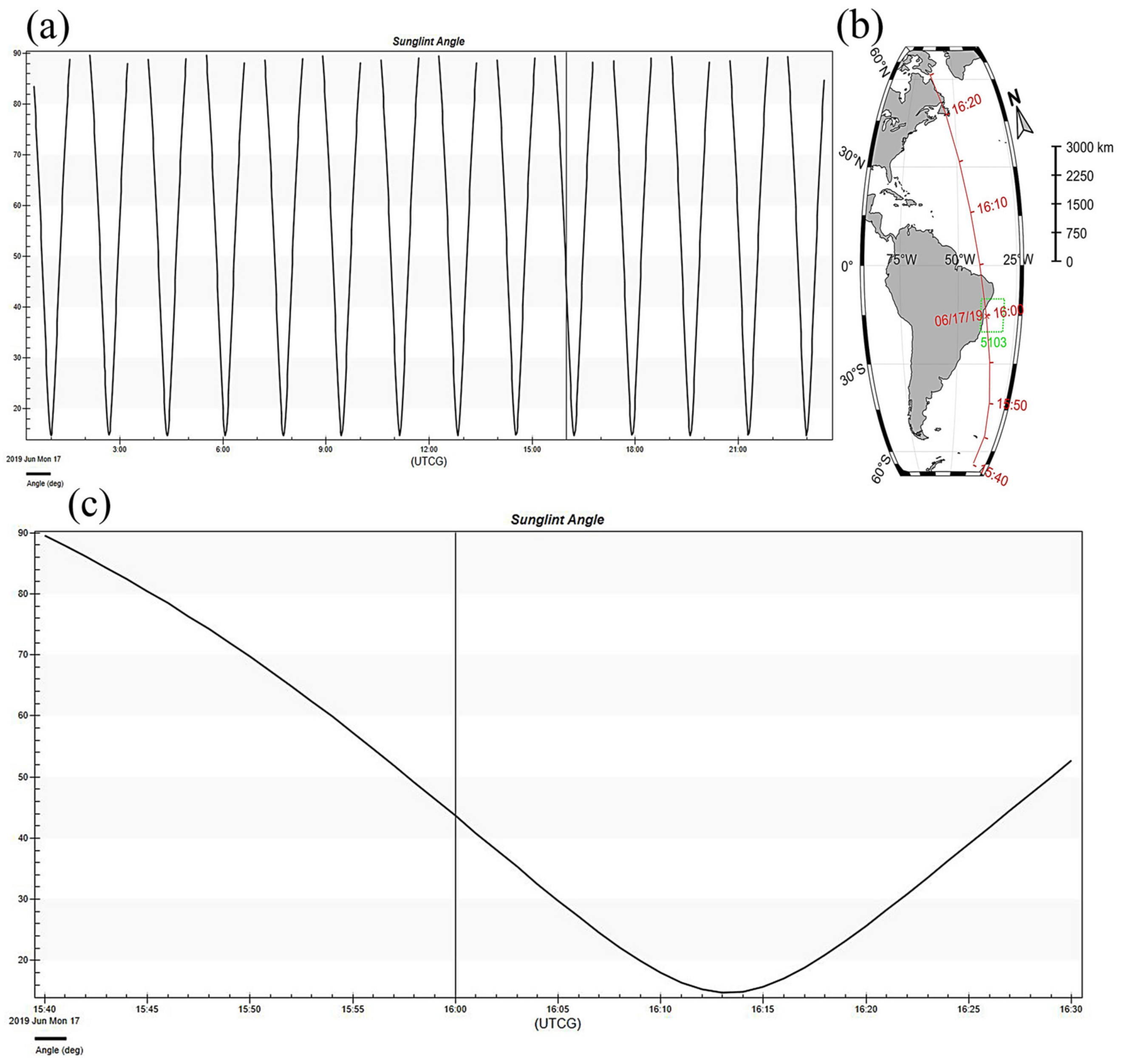
5.1. Simulation of Sun-Glint Locations and Zenith Angles

The GAS payload was carried for the first time on the FengYun-3D satellite, which has operated normally in orbit. Both FY-3D and FY-3H are in sun-synchronous orbit. Therefore, the sun-glint position of the first-generation GAS was used in the following article, and the instrument parameters were updated to the next-generation in the simulation.

Here, the FY-3D satellite orbital parameters are imported into Systems Tool Kit (STK) software to generate the real-time position of the sun glint and the solar zenith angle at different times. The selected time period spanned from 15:42 to 16:20 on 17 June 2019, when the GAS sun-glint position shifted from north of Antarctica in the Southwest Atlantic to the sea west of Canada in the Northwest Atlantic. The position and angle information of the sun glint at each moment are shown in

Table 1. GAS sun-glint locations and zenith angles on 17 June 2019.

Time (UTCG)	Detic Latitude (deg)	Detic Longitude (deg)	Solar Zenith Angle of the Sun Glint (°)	Solar Zenith Angle of the Observer (°)
2019/6/17 15:42	−60.492	−32.266	86.097	118.385
2019/6/17 15:45	−54.053	−31.452	80.454	119.605
2019/6/17 15:50	−42.249	−32.475	69.69	124.232
2019/6/17 15:51	−39.708	−32.873	67.327	125.564
2019/6/17 15:52	−37.108	−33.313	64.898	127.027
2019/6/17 15:54	−31.734	−34.29	59.856	130.316
2019/6/17 15:56	−26.15	−35.363	54.6	134.038
2019/6/17 15:58	−20.382	−36.508	49.177	138.117
2019/6/17 15:59	−17.438	−37.102	46.42	140.265
2019/6/17 16:00	−14.459	−37.71	43.642	142.47
2019/6/17 16:01	−11.45	−38.329	40.852	144.721
2019/6/17 16:05	0.834	−40.935	29.798	153.918
2019/6/17 16:08	10.217	−43.054	22.146	160.478
2019/6/17 16:10	16.512	−44.576	17.932	164.148
2019/6/17 16:15	32.237	−48.988	15.674	166.247
2019/6/17 16:20	47.672	−55.087	25.669	157.627

. The variation pattern of sun-glint zenith angle during the day and the distribution of sun-glint positions on the map are shown in Figure A4.

We selected the sun-glint location in the sea west of Salvador city, Brazil, in the South Atlantic Ocean at 16:00 on 17 June 2019; this site is located in the World Meteorological Organization (WMO) SQUARES 5103 zone. The satellite observation zenith angle at this moment was 142.358°. The integrated meteorological dataset of the sea-surface database shows that within ±1 h and 1° × 1°, the temperature in the sea area at that time was 29 °C, the sea level pressure was 1014 mbar, the average sea-surface visibility was 20 km, the wind speed was 8.7 m/s, and the 24 h average wind speed was 7.29 m/s [51]. Although the location of this sun glint was relatively close to the South American continent, the influence of land-based air masses on the sea was limited by atmospheric circulation, and the city of Salvador has a low industrial level, so we set the ICSTL to 6.

5.2. Simulation of Wind-Driven Rough-Sea-Surface Reflectivity

We showed in Section 3.4 that the sea-surface reflectance is mainly determined by a combination of the solar zenith angle at the sun-glint point and the sea-surface wind speed. Therefore, the improved Cox–Munk-based model detailed in Section 3.4 was used to calculate the reflectance of solar shortwave infrared radiation propagating over a rough sea surface. Compared to other reflectivity models, this model takes into account the depolarization of the sea surface as well as the sea-surface roughness in the absence of wind. Since the incident solar light is nonpolarized, only the zenith angle of the incident direction is considered in the calculation.

From the simulation results (Figure 2), the overall reflectivity was found to increase with an increasing incident zenith angle. In the low-incidence-angle region (θ < 40°), the effect of the wind speed is not obvious, and the variation in the overall reflectivity is relatively small. In the high-incidence-angle region (θ > 60°), the reflectivity increases rapidly with an increasing incident zenith angle, and the higher the wind speed is, the higher the roughness of the sea surface is and the lower the reflectivity is.

The wind speed of 8.7 m/s and the sun-glint zenith angle of 43.642° at 16:00 on 17 June 2019 were input to the model to obtain the sea-surface reflectivity of 0.0291 at that time [51]. In addition, the parameters of different sea areas in Section 5.4.2 were input to the model, and the corresponding sea-surface reflectance was obtained; the reflectance is marked with dots of different colors in Figure 2.

5.3. Simulations under Different Instrumental Parameters

5.3.1. Spectral Resolution

The U.S. Standard Atmosphere 1976 [52] model was used in the simulation calculations, and multiple resolutions were established for comparison. In the 1.61 μm band, the CO₂ absorption line width of 0.07 cm⁻¹ in the 1.61 μm spectrum was used as the reference standard for the spectral resolution, and 0.482 cm⁻¹ (the ACGS spectral resolution), 0.308 cm⁻¹ (the OCO-3 spectral resolution), and 0.27 cm⁻¹ (the GAS spectral resolution) were compared with the results to analyze the variation characteristics of the CO₂ absorption spectrum. In the 2.06 μm spectral band, 0.07 cm⁻¹ was also used as a reference standard, and 0.388 cm⁻¹ (the ACGS spectral resolution), 0.236 cm⁻¹ (the OCO-3 spectral resolution), and 0.212 cm⁻¹ (the GAS spectral resolution) were applied for comparison. To eliminate the effect of the spectral sampling rate, the sampling rate was set to 8. The detailed input model parameters are shown in

Table A2. Detailed input parameters for model Settings.

Simulation of Indicator	Parameter
Atmospheric model	U.S. Standard Atmosphere 1976
Wavenumber range/cm−1	6150–6290; 4806–4902
Aerosol type	Maritime
Real-time sea-surface wind speed	8.7 m/s
24 h average sea-surface wind speed	7.29 m/s
ICSTL	6
Sea-surface temperature	300.2 K
Sea-surface visibility	20 km
Solar zenith angle of the observer	142.358°
Solar zenith angle of the sun glint	43.642°
Sea-surface reflectivity	0.0291

.

The LBLRTM has a spectral resolution of 0.0014 cm⁻¹. In the simulation, a Gaussian-type function is used to simulate the slit function of the grating spectrometer as a line function of the LBLRTM instrument to convolve with the original spectrum to obtain the required transmittance spectrum and bright temperature spectrum at the spectral resolution designated above.

From the simulation results, the CO₂ transmittance spectrum exhibits a clear double-peak structure in the 1.61 μm band and from left to right for the P-branch and R-branch, respectively. At a spectral resolution of 0.07 cm⁻¹, the wavenumbers of the two branches are approximately 6228 cm⁻¹, and the local nadir transmittance values are 6216 cm⁻¹ and 6239 cm⁻¹, respectively. The 2.06 μm spectrum also exhibits a certain bimodal structure, with local minima of transmittance at 4842 cm⁻¹ and 4865 cm⁻¹ and two branching wavenumbers at 4854 cm⁻¹. Since this spectrum is a strong CO₂ absorption band, the overall transmittance is significantly reduced compared to the 1.61 μm spectrum.

From the comparison in Figure 3, it can be seen that the overall transmittance decreases as the spectral resolution increases in both spectral bands, and the double-peak structure is more obvious. In the 2.06 μm spectrum, the AGAS instrument differs from other instruments due to its relatively large spectral resolution, and the wavenumber where the lowest transmittance point is located is also shifted. The brightness temperature simulation results are similar to the transmittance results. The specific data corresponding to each spectral nadir are shown in

Table A3. Transmittance and brightness temperature at spectral nadir of the 1.6 μm spectral band.

Payload		CO2 Absorption	GAS	OCO-3	AGAS
Spectral resolution		0.07 cm−1	0.27 cm−1	0.308 cm−1	0.482 cm−1
Transmittance spectrum	P-branch Tmin (6216 cm−1)	0.3279	0.5848	0.6025	0.6709
	R-branch Tmin (6239 cm−1)	0.3028	0.5738	0.5897	0.6578 (6241 cm−1)
Brightness temperature spectrum	P-branch BTmin (6216 cm−1)	288.8 K	295.1 K	295.4 K	296.5 K
	R-branch BTmin (6239 cm−1)	288.1 K	295.0 K	295.3 K	296.3 K (6241 cm−1)

and

Table A4. Transmittance and brightness temperature at spectral nadir of the 2.06 μm spectral band.

Payload		CO2 Absorption	GAS	OCO-3	AGAS
Spectral resolution		0.07 cm−1	0.212 cm−1	0.236 cm−1	0.388 cm−1
Transmittance spectrum	P-branch Tmin (4842 cm−1)	0.00036	0.05783	0.07688	0.19353
	R-branch Tmin (4865 cm−1)	0.00017	0.064857	0.040283	0.14792 (4862 cm−1)
Brightness temperature spectrum	P-branch BTmin (4842 cm−1)	242.7 K	270.3 K	272.9 K	281.9 K
	R-branch BTmin (4865 cm−1)	242.3 K	268.7 K	271.4 K	279.7 K

.

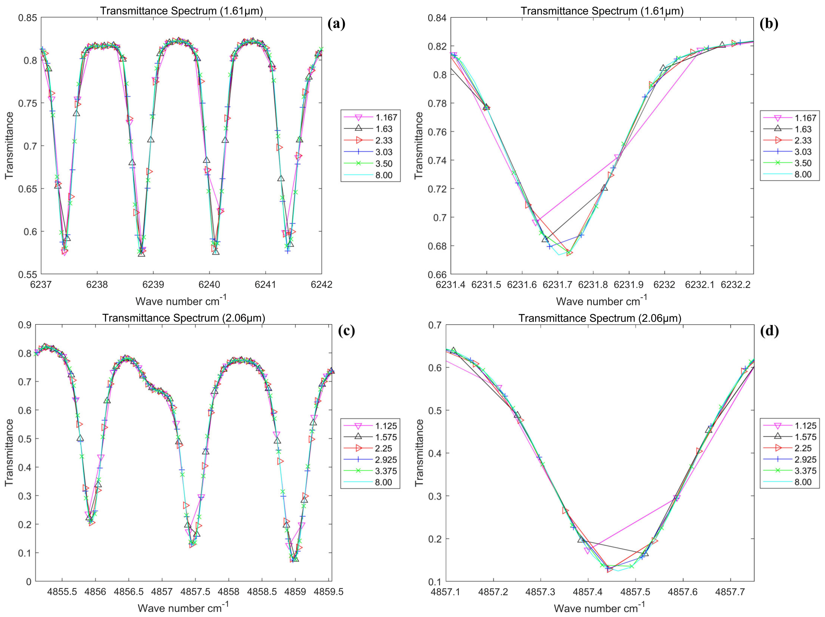
5.3.2. Spectrum Sampling Rate

In the simulation calculations performed in this subsection, considering that the actual spectral width of the instrument is limited by the optical spectroscopic system, the actual design index of GAS is substituted into the model as follows: the 1.61 μm spectral band with a spectral width of 30 nm and a spectral resolution of 0.27 cm⁻¹ and the 2.06 μm spectral band with a spectral width of 40 nm and a spectral resolution of 0.212 cm⁻¹. Moreover, in this paper, the detector is abstracted as an array of image elements in the simulations, and the difference in the actual performance of the detector is not considered. The actual performance difference and the effect of the spatial dimension are thus not considered. Only the comparative transmittance spectra are simulated in this subsection.

Five detectors with 500, 700, 1000, 1300, and 1500 spectral-dimensional elements are used as examples. In the 1.61 μm spectral band, five spectral sampling rates of 1.167, 1.63, 2.33, 3.03, and 3.5 are represented; in the 2.06 μm spectral band, five spectral sampling rates of 1.125, 1.575, 2.25, 2.925, and 3.375 are represented. The sampling rate of 8 was used as the reference standard for comparisons of both spectral bands. The rest of the parameters were set to be the same as those listed in Table A2.

The comparison in Figure 4 shows that the larger the spectral sampling rate is, the finer the peak structure of the CO₂ absorption line obtained by the instrument is. As Figure 4b shows, the spectral sampling rates of 1.167 and 1.63 do not meet the theoretical requirement of being no less than 2, there is an obvious problem of undersampling, and the bottom of the peak structure is not sampled properly, causing some spectral information to be missing. In Figure 4c, the two spectral sampling rates of 1.125 and 1.575 also show similar problems. When the spectral sampling rate is greater than 2, no significant difference occurs in the fineness of the CO₂ absorption lines shown in the figure.

5.4. Simulations under Different Environmental Parameters

In this section, the GAS design parameters were applied as the instrumental parameters to simulate the CO₂ observation spectra in the sea-surface environment to study the GAS capability of detecting CO₂ in different sea areas. The spectral resolution was 0.27 cm⁻¹ in the 1.61 μm band at a spectral sampling rate of 3.3; in the 2.06 μm band with a spectral sampling rate of 3.4, the spectral resolution was 0.212 cm⁻¹.

5.4.1. Different Wind Speeds and Visibilities

As described previously in Section 3.2, visibility and wind speed are the main parameters required when assessing the extinction and absorption effects of ocean-type aerosols; the wind speed in particular additionally affects the sea-surface conditions. In this paper, the effects of these two parameters on the CO₂ detection spectrum were investigated first. Since it is difficult to model a realistic situation in which only the wind speed or visibility differs at the sun-glint location while all other parameters remain consistent, simulations in this subsection are performed only for comparisons of abstract sun-glint conditions.

Six different wind speeds of 0.1, 2, 3, 5, 7, and 15 m/s were selected for simulation and comparison, assuming that the 24 h average wind speed was the same as the real-time wind speed. The visibility was fixed at 20 km, the sun-glint zenith angle was fixed at 40°, and the corresponding sea-surface reflectance values were 0.0247, 0.0251, 0.0253, 0.0257, 0.0261, and 0.0268. The simulated visibility was selected from five different VIS values of 5, 7, 15, 25, and 50 km for the simulations, and the wind speed was fixed at 7 m/s. The remaining parameters were the same as those listed in Table A2.

From Figure 5a,c, it can be seen that the transmittance spectra of both spectral bands decreased with increasing wind speeds. From Equations (3) and (4), it can be seen that the wind speed is proportional to the attenuation and absorption coefficients; a decrease in radiant energy occurs with an increase in wind speed, which is consistent with the simulation results. In the 1.61 μm spectrum, the wind speed increases from 0.1 m/s to 5 m/s, and the transmittance spectrum decreases greatly; the transmittance spectrum decreases relatively less when the wind speed is above 5 m/s. In the 2.06 μm spectral band, the effect of the wind speed is similar to that obtained in the 1.61 μm spectral band.

Figure 5b,d illustrates that the transmittance spectra of both spectral bands decrease with decreasing visibility. According to the aerosol absorption principle, the visibility is inversely proportional to the aerosol attenuation coefficient [53], corresponding to a decrease in radiant energy with a decrease in visibility; this finding is consistent with the simulation results. Similar to the wind speed simulation results, when the visibility decreases, the decrease in the 1.61 μm spectrum is more obvious than that in the 2.06 μm spectrum.

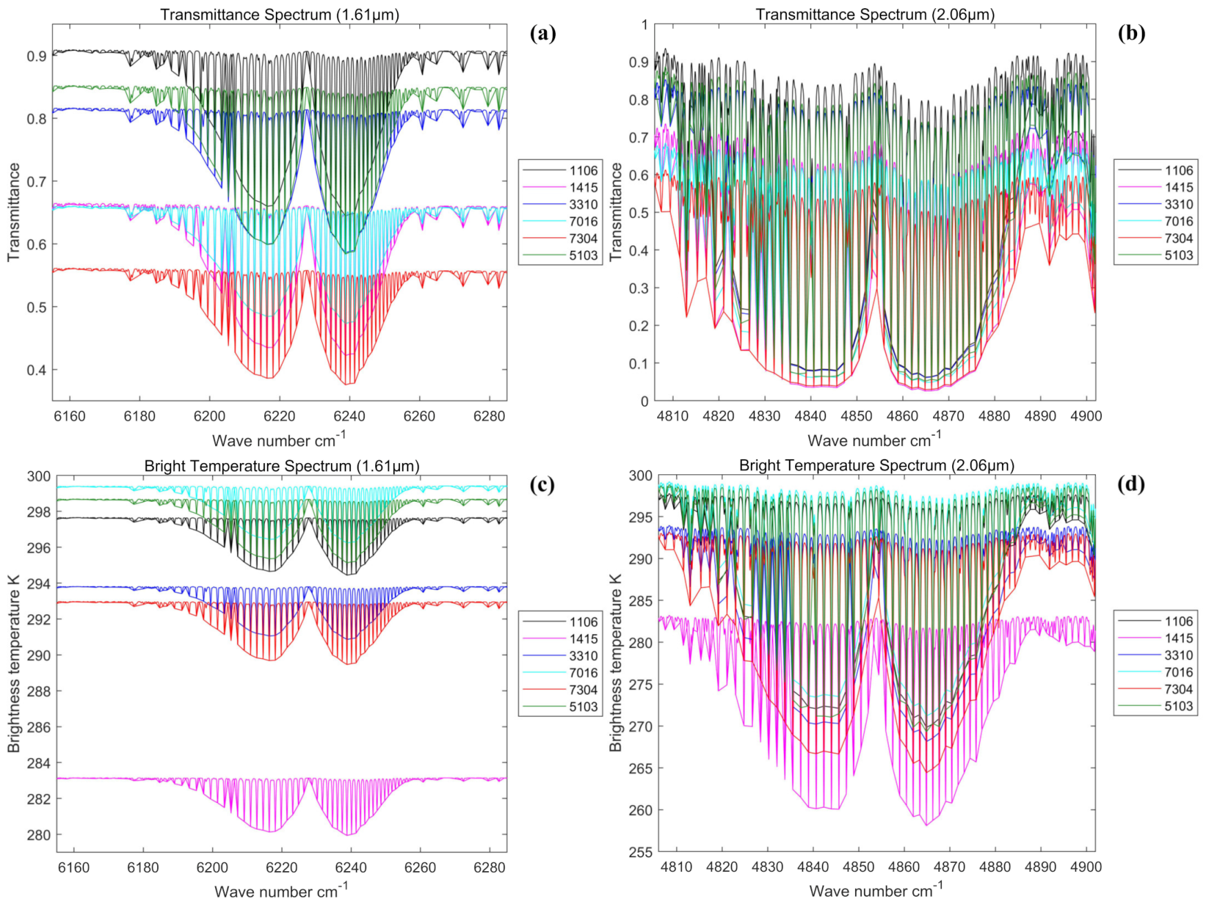
5.4.2. Different Sea Areas

Six GAS sun-glint scenarios distributed in different global oceans were selected and compared, as shown in Figure 6. From

Table 2. Model parameters in different sea areas at various times [51].

WMO SQUARE	7016	1106	1415	3310	7304	5103
Longitude (°)	(160,170) W	(60,70) E	(150,160) E	(100,110) E	(40,50) W	(30,40) W
Latitude (°)	(0,10) N	(10,20) N	(40,50) N	(30,40) S	(30,40) N	(10,20) S
Time (UTCG)	2019/6/30 0:06:00	2019/2/23 8:42:00	2019/11/4 1:58:00	2019/2/2 6:42:00	2019/10/18 15:50:00	2019/6/17 16:00:00
Sun-glint position	(4.08°N, 161.59°W)	(18.534°N, 66.611°E)	(44.87°N, 156.438°E)	(31.567°S, 104.739°E)	(37.746°N, 47.067°W)	(14.459°S, 37.71°W)
AT (K)	303.3	298.6	283.3	295.4	297.2	300.2
WSS (m/s)	2.6	6.7	3.1	10.3	10.8	8.7
WHH (m/s)	2.35	6.308	9.58	9.91	8.98	7.29
VIS (km)	10	20	10	20	10	20
SZA of the sun glint (°)	26.501	31.598	61.02	24.744	49.402	43.642
Sea-surface reflectivity	0.0212	0.0225	0.0665	0.0215	0.0355	0.0291
SZA of the observer (°)	156.730	152.471	129.452	158.370	137.947	142.470
ICSTL	1	9	7	3	2	6

and Figure 7, it can be seen that the environmental parameters in the sea areas where the sun glints were located at different times varied greatly and significantly affected the transmittance and bright temperature spectra received by the instruments. Similar to the results described in Section 5.4.1, the transmittance spectra are mainly affected by the wind speed and visibility. The wind speed is the highest and visibility is the lowest in sea area 7304, and in this area, the transmittance in the two spectral bands is also significantly lower than in other sea areas; the situation is the opposite in sea area 1106. Among the sea areas, the benchmark of the bright temperature spectra depends mainly on the air temperature over the sea surface and visibility level. For example, sea area 1415 is located in a mid-winter spatial and temporal zone, and the air temperature over the sea surface in this area is relatively low compared to other sun-glint sites, so the bright temperature spectrum also decreases accordingly. Therefore, to obtain accurate sea-surface CO₂ concentrations, it is necessary to improve the accuracy of the sea-surface environmental parameters. The overall spectral contrasts between the two spectral bands are similar with regards to different environmental parameters in the sea areas.

In the table above, AT indicates the air temperature, SZA indicates the solar zenith angle, and “WMO SQUARES” is a geographical code system that divides the global map and latitude longitude grid lines into grid cells each of 10° latitude by 10° longitude. Each grid cell has a unique four-digit numeric identifier [54,55].

5.4.3. Rough Sea Surface

As described in Section 3.2, the magnitude of the rough-sea-surface reflectivity is affected by both the wind speed and sun-glint solar zenith angle. In this section, the differences in the spectra of the radiance received by the instruments are studied in two cases: one considering the wind-driven rough-sea-surface model and one not considering this model. In

Table 3. Reflectance of the rough sea surface under six different wind speeds and sun-glint conditions.

WSS (m/s)	7	7	10	10	12	12
SZA of the sun glint (°)	60	65	65	70	75	80
Reflectivity	0.060	0.080	0.0745	0.0984	0.1246	0.1693

, six different wind speed and sun-glint cases were selected to illustrate the effect of the rough-sea-surface reflectivity compared to a general sea-surface reflectivity of 0.025.

From Figure 8, it can be seen that in the case of a large sun-glint zenith angle (>60°), if the change in the reflectivity of the rough sea surface is not considered, this omission will cause a large simulation error in the radiance spectrum received by the instrument and thus affect the accuracy of the subsequent CO₂ inversion results.

6. Discussion

6.1. Evaluation of the Detection Accuracies at Different Spectral Resolutions

The absolute deviation of the GAS instrument between the 1.61 μm and 2.06 μm bands is shown in Figure 9, and the detection accuracy evaluation indices are shown in

Table 4. Detection accuracy index corresponding to each spectral resolution in the 1.61 μm band.

	Payload	SR (cm−1)	Nmp	RMSE	MAXAD	MAXAPD (%)	MAD	MAPD (%)
Tr	GAS	0.27	4119	0.0304	0.2644	85.45	0.0104	1.74
	OCO-3	0.308	3707	0.0329	0.2873	94.89	0.0114	1.90
	ACGS	0.482	2308	0.0422	0.3571	116.91	0.0160	2.62
BT	GAS	0.27	4119	0.5251 K	5.7100 K	1.97	0.1507 K	5.103 × 10−2
	OCO-3	0.308	3707	0.5620 K	6.1735 K	2.14	0.1638 K	5.548 × 10−2
	ACGS	0.482	2308	0.6921 K	7.1785 K	2.48	0.2209 K	7.475 × 10−2

and

Table 5. Detection accuracy index for each spectral resolution in the 2.06 μm band.

	Payload	SR (cm−1)	Nmp	RMSE	MAXAD	MAXAPD (%)	MAD	MAPD (%)
Tr	GAS	0.212	3623	0.0469	0.2390	2.807 × 104	0.0320	111.37
	OCO-3	0.236	3254	0.0538	0.2740	2.531 × 104	0.0372	134.31
	ACGS	0.388	1979	0.0906	0.3800	5.332 × 104	0.0654	292.68
BT	GAS	0.212	3623	4.3469 K	28.501 K	11.71	1.5292 K	0.57
	OCO-3	0.236	3254	4.7765 K	30.526 K	12.54	1.7132 K	0.64
	ACGS	0.388	1979	6.4635 K	39.107 K	16.07	2.5352 K	0.94

. From the results listed in Table 4 and Table 5, it can be seen that the higher the spectral resolution and thus the more data points the instrument receives that the transmittance spectrum and bright temperature spectrum can then match with the reference spectrum, the lower the absolute deviation index of both results is and the lower the RMSE is. This finding also indicates that the overall simulation spectral curve is relatively close to the reference spectrum. Among the grating spectrometers, the spectral resolution of the new-generation GAS is at the international level, and the spectral deviation indices corresponding to the 1.61 μm and 2.06 μm spectral bands are also the smallest among similar instruments.

In the table above, Tr represents transmittance, BT represents the brightness temperature, SR represents the spectral resolution, and N_mp represents the number of matching points, which is equal to the number of data points for which the wavenumber difference between the current transmittance spectrum and the reference spectrum is less than 0.035 cm⁻¹.

6.2. Evaluation of Detection Accuracies under Different Spectral Sampling Rates

The absolute deviation of the 1300-image scale detector in the 1.61 μm spectral band from the 2.06 μm spectral band is shown in Figure 10, and the detection accuracy evaluation indices are shown in

Table 6. Results obtained for the 1.61 μm spectral band at different spectral sampling rates of the transmittance spectral accuracy index.

SSR	RMSE	MAXAD	MAXAPD (%)	MAD	MAPD (%)
1.167	0.0086	0.0667	11.50	0.0035	0.49
1.63	0.0047	0.0409	6.98	0.0018	0.25
2.33	0.0024	0.0202	3.49	8.791 × 10−4	0.12
3.03	0.0014	0.0138	2.40	4.980 × 10−4	0.069
3.50	0.0010	0.0110	1.92	3.536 × 10−4	0.049

In the table above, SSR indicates the spectral sampling rate.

and

Table 7. Results obtained for the 2.06 μm spectral band at different spectral sampling rates of the transmittance spectral accuracy index.

SSR	RMSE	MAXAD	MAXAPD (%)	MAD	MAPD (%)
1.125	0.0226	0.1157	150.24	0.0148	5.14
1.575	0.0121	0.0621	71.33	0.0078	2.71
2.25	0.0059	0.0295	36.09	0.0038	1.31
2.925	0.0034	0.0173	19.92	0.0022	0.74
3.375	0.0025	0.0133	14.84	0.0016	0.54

. From Table 6 and Table 7, it can be seen that as the spectral sampling rate increases, the absolute deviation of the instrument transmittance spectrum decreases accordingly, the RMSE decreases, and the fit of the detection spectrum increases. Compared to the spectral resolution results, the influence of the spectral sampling rate on the accuracy of the detection spectrum is approximately an order of magnitude smaller. Considering the detector-production process, the detector image element should prioritize ensuring that the spectral resolution of the instrument can reach the design level before considering increasing the spectral sampling rate. Generally, when the spectral sampling rate reaches 3, the spectral MAPD is less than 1%, which can meet the high sampling accuracy required; thus, the GAS instrument meets this condition.

6.3. Evaluation of the Detection Accuracies Obtained under Different Wind Speeds and Visibility Levels within the Simulated Spectra

In this section, the reference standard of wind speed is 0.1 m/s, and the difference indices obtained under different wind speeds are shown in

Table 8. Differences index in transmittance spectra at different wind speeds.

	WSS (m/s)	RMSE	MAXAD	MAXAPD (%)	MAD	MAPD (%)
1.61 μm spectral band	0.1	0	-	-	-	-
	2	0.0055	0.0057	0.6148	0.0055	0.6147
	3	0.0513	0.0528	5.7529	0.0512	5.7176
	5	0.0963	0.0993	10.8067	0.0961	10.7359
	7	0.1126	0.1161	12.6346	0.1124	12.5523
	15	0.1336	0.1377	14.9897	0.1334	14.8986
2.06 μm spectrum band	0.1	0	-	-	-	-
	2	0.0050	0.0066	0.6997	0.0048	0.6978
	3	0.0358	0.0466	5.0370	0.0341	4.9873
	5	0.0663	0.0862	9.3265	0.0630	9.2277
	7	0.0775	0.1008	10.9082	0.0737	10.7931
	15	0.0932	0.1212	13.1070	0.0887	12.9781

. Figure 11 shows the RMSE and MAPD curves and their change rates in the wind speed range of 0.1–25 m/s under the two analyzed spectral bands. From Table 8 and Figure 11, it can be seen that the transmittance spectrum decreases as the wind speed increases. When the wind speed is less than 2.2 m/s, the influence of the wind speed on the transmittance spectrum is less than 0.7%, and the variation trend with the wind speed is not obvious. In the wind speed range from 2.2 m/s to 5 m/s, the transmittance spectrum changes abruptly with the wind speed, and the decline rate increases significantly. When the wind speed increases to more than 5 m/s, the difference in transmittance spectra becomes more obvious, and the spectral effect introduced by the wind speed needs to be considered in the simulation. When the wind speed exceeds 20 m/s, the effect of a further wind speed change on the transmittance spectra tends towards 0.

The reference standard of visibility was set to 50 km, and the different index values obtained under different visibility conditions are shown in

Table 9. Differences index in transmittance spectra at different visibilities.

	VIS (km)	RMSE	MAXAD	MAXAPD (%)	MAD	MAPD (%)
1.61 μm spectral band	50	0	-	-	-	-
	25	0.0747	0.0772	8.3902	0.0746	8.3173
	15	0.1754	0.1811	19.6810	0.1752	19.5339
	7	0.3746	0.3862	41.9733	0.3741	41.7112
	5	0.4773	0.4917	53.4362	0.4766	53.1544
2.06 μm spectrum band	50	0	-	-	-	-
	25	0.0483	0.0628	6.8248	0.0460	6.7547
	15	0.1171	0.1522	16.5253	0.1114	16.3681
	7	0.2588	0.3358	36.4654	0.2461	36.1677
	5	0.3351	0.4350	47.1845	0.3187	46.8365

. Figure 12 shows the RMSE and MAPD curves and their change rates in the visibility range of 5–50 km under the analyzed two spectral bands. As seen from Table 9 and Figure 12, the instrument transmittance spectrum decreases overall as the visibility decreases. The variation in transmittance is larger in the visibility range of 5–10 km and smaller in the >20 km range. The influence of visibility in the 2.06 μm band is slightly smaller than that in the 1.61 μm band, and the overall variations in transmittance in the two bands are very similar.

6.4. Evaluation of the Detection Accuracies Obtained under Different Rough-Sea-Surface Conditions

Table 10. Differences index in radiance spectra at different reflectivities.

WSS (m/s)	SZA of the sun glint (°)	Reflectivity	Spectral Band	RMSE (W·m−2sr−1 cm−1)	MAD (W·m−2sr−1 cm−1)	MAPD (%)
7	60	0.0600	1.61 μm	6.785 × 10−13	6.624 × 10−13	1.2762
			2.06 μm	4.150 ×10−10	3.757 × 10−10	1.7266
7	65	0.0800	1.61 μm	2.320 × 10−12	2.268 × 10−12	4.5303
			2.06 μm	8.454 × 10−10	7.674 × 10−10	3.6585
10	65	0.0745	1.61 μm	2.361 × 10−12	2.308 × 10−12	4.6148
			2.06 μm	8.637 × 10−10	7.864 × 10−10	3.7633
10	70	0.0984	1.61 μm	5.233 × 10−12	5.116 × 10−12	10.8831
			2.06 μm	1.916 × 10−9	1.747 × 10−9	8.9576
12	75	0.1246	1.61 μm	7.940 × 10−12	7.761 × 10−12	17.5713
			2.06 μm	2.890 × 10−9	2.628 × 10−9	14.3476
12	80	0.1693	1.61 μm	1.519 × 10−11	1.485 × 10−12	40.2094
			2.06 μm	6.282 × 10−9	5.711 × 10−9	38.7185

shows the deviation index between the reflectivity of various rough sea surfaces and the reflectivity of 0.025. As seen from Table 10, in the case of a high sun-glint zenith angle (>60°), the rough-sea-surface reflectivity is much larger than the general sea-surface reflectivity (0.025), and this difference has a strong effect on the radiance spectrum received by the instrument. Among the analyzed conditions, the instrument radiance spectrum MAPD is greater than 3% for zenith angles >65° and greater than 10% for zenith angles >75°. The effect of the rough-sea-surface conditions in the 2.06 μm spectral band is relatively small compared to that in the 1.61 μm spectral band, and the MAPD difference between these two bands reaches a maximum value of 3.2237% at a reflectivity of 0.1246. According to STK statistics, 43.13% of the GAS sun-glint zenith angles were greater than 60° in 2019. In this case, we must consider the effect of rough-sea-surface conditions; otherwise, the CO₂ detection accuracy would be seriously affected.

7. Conclusions

In this study, we simulated the high-spectral absorption spectra in two bands (strong and weak) of atmospheric CO₂ molecules, taking into account both the effects of different instrumental parameters (the spectral resolution and spectral sampling rate) and environmental parameters (the wind speed, visibility, and rough sea surface) above the sea. The model was improved by considering the effects of marine aerosols, the wind-driven rough-sea-surface reflectivity, and the sea-surface sun-glint model. The preliminary results show that, using CO₂ molecular absorption spectroscopy as a benchmark for verification, the RMSE of GAS’s atmospheric CO₂ detection transmittance spectra is within 0.031, and the MAD is within 0.011 in the 1.61 μm band; in addition, the RMSE is within 0.05, and the MAD is within 0.033 in the 2.06 μm band. These results reveal that GAS is competitive among similar CO₂ instruments. The main conclusions of this work are described as follows:

(1)

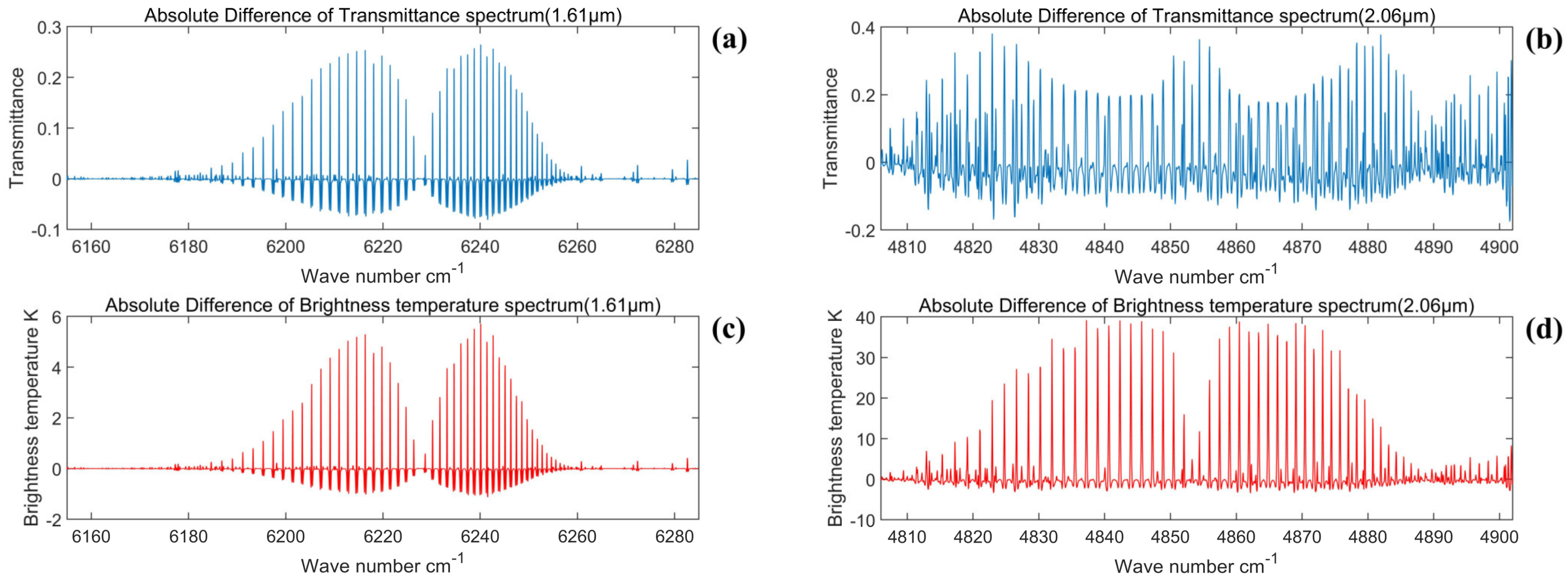
The higher the spectral resolution of an instrument is, the richer the received detection spectral information is, the lower the absolute deviation index is, the lower the RMSE is, and the closer the overall simulated spectral curve is to the real spectrum. The spectral resolution of the new-generation GAS instrument is at a leading level internationally, and the spectral deviation index values obtained for the 1.61 μm and 2.06 μm spectral bands are smallest among similar existing instruments;

(2)

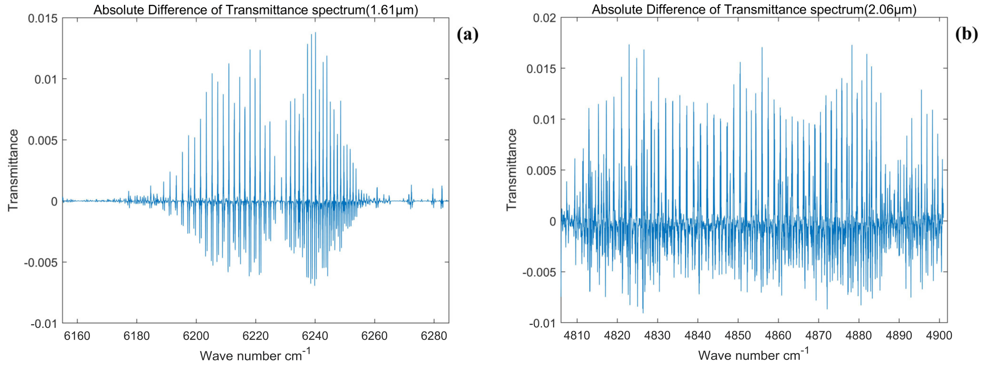
The higher the spectral sampling rate of the instrument is, the smaller the absolute deviation of the detection spectrum and the lower the RMSE are. Compared to the effect of the spectral resolution, the impact of the spectral sampling rate on the accuracy of the detection spectrum is approximately an order of magnitude smaller. In the actual instrument design, the detector image element should prioritize ensuring that the instrumental spectral resolution can reach the design level before considering increasing the spectral sampling rate. Generally, a spectral sampling rate of 3 is appropriate;

(3)

The higher the wind speed of the sea-surface atmosphere is, the lower the overall instrument detection spectrum is. When the wind speed is less than 2 m/s, the effect of the transmittance spectrum introduced by the wind speed is less than 0.02% and can thus be ignored. When the wind speed is above 5 m/s, the difference in transmittance spectra is more obvious, and the spectral effects introduced by the wind speed must be considered in the simulations;

(4)

The greater the atmospheric visibility of the sea surface is, the lower the overall instrument detection spectrum is. The variation in transmittance is larger in the 5–10 km visibility range; at visibilities above 20 km, the variation in transmittance is relatively low. The overall transmittance trends in the 2.06 μm and 1.61 μm spectral bands were similar, and the former was relatively less affected by visibility;

(5)

Approximately 43% of the sun-glint zenith angles were > 60° during the study period. Under these conditions, it is important to consider the change in the reflectivity of the rough sea surface; otherwise, the CO₂ detection accuracy will be seriously affected.

In general, in this work, we simulated and analyzed the effects of instrumental parameters and atmospheric-environmental parameters as well as the bottom-boundary effect of the rough sea surface on the spectral information received by the GAS instrument. These results are expected to provide a reference for the design of greenhouse gas hyperspectral detection instruments and contribute to the spectral data processing of CO₂ in the above-sea atmosphere. In the future, our model will be investigated in more times and sea areas. Meanwhile, more and newer atmospheric modes will be used in our model to test the effects of location and season.

References

1. Kuttippurath, J.; Peter, R.; Singh, A.; Raj, S. The increasing atmospheric CO2 over India: Comparison to global trends. Iscience 2022, 25, 104863. [Google Scholar] [CrossRef] [PubMed]
2. Liu, Y.; Wang, J.; Yao, L.; Chen, X.; Cai, Z.; Yang, D.; Yin, Z.; Gu, S.; Tian, L.; Lu, N.; et al. The TanSat mission: Preliminary global observations. Sci. Bull. 2018, 63, 1200–1207. [Google Scholar] [CrossRef] [Green Version]
3. Schwandner, F.M.; Gunson, M.R.; Miller, C.E.; Carn, S.A.; Eldering, A.; Krings, T.; Verhulst, K.R.; Schimel, D.S.; Nguyen, H.M.C.; David, O.; et al. Spaceborne detection of localized carbon dioxide sources. Science 2017, 358, eaam5782. [Google Scholar] [CrossRef] [PubMed] [Green Version]
4. Kiehl, J.T. Satellite detection of effects due to increased atmospheric carbon dioxide. Science 1983, 222, 504–506. [Google Scholar] [CrossRef] [PubMed]
5. Baker, D.F.; Boesch, H.; Doney, S.C.; O'Brien, D.; Schimel, D.S. Carbon source/sink information provided by column CO2 measurements from the Orbiting Carbon Observatory. Atmos. Chem. Phys. 2010, 10, 4145–4165. [Google Scholar] [CrossRef] [Green Version]
6. Chatterjee, A.; Gierach, M.M.; Sutton, A.J.; Feely, R.A.; Crisp, D.; Eldering, A.; Gunson, M.R.; O’Dell, C.; Stephens, B.B.; Schimel, D.S. Influence of El Ni?o on atmospheric CO2 over the tropical Pacific Ocean: Findings from NASA’s OCO-2 mission. Science 2017, 358, eaam5776. [Google Scholar] [CrossRef] [Green Version]
7. Miller, J.B.; Tans, P.P.; Gloor, M. Steps for success of OCO-2. Nat. Geosci. 2014, 7, 691. [Google Scholar] [CrossRef]
8. Sun, Y.; Frankenberg, C.; Wood, J.D.; Schimel, D.S.; Jung, M.; Guanter, L.; Drewry, D.T.; Verma, M.; Porcar-Castell, A.; Griffis, T.J.; et al. OCO-2 advances photosynthesis observation from space via solar-induced chlorophyll fluorescence. Science 2017, 358, eaam5747. [Google Scholar] [CrossRef] [Green Version]
9. Heffernan, O. NASA’s next challenge. Nat. Clim. Change 2009, 1, 28. [Google Scholar] [CrossRef] [Green Version]
10. Butz, A.; Guerlet, S.; Hasekamp, O.; Schepers, D.; Galli, A.; Aben, I.; Frankenberg, C.; Hartmann, J.M.; Tran, H.; Kuze, A. Toward accurate CO2 and CH4 observations from GOSAT. Geophys. Res. Lett. 2011, 38, L14812. [Google Scholar] [CrossRef]
11. Guanter, L.; Frankenberg, C.; Dudhia, A.; Lewis, P.E.; Gómez-Dans, J.; Kuze, A.; Suto, H.; Grainger, R.G. Retrieval and global assessment of terrestrial chlorophyll fluorescence from GOSAT space measurements. Remote Sens. Environ. 2012, 121, 236–251. [Google Scholar] [CrossRef]
12. Frankenberg, C.; Fisher, J.B.; Worden, J.; Badgley, G.; Saatchi, S.S.; Lee, J.E.; Toon, G.C.; Butz, A.; Jung, M.; Kuze, A. New global observations of the terrestrial carbon cycle from GOSAT: Patterns of plant fluorescence with gross primary productivity. Geophys. Res. Lett. 2011, 38, L17706. [Google Scholar] [CrossRef] [Green Version]
13. Yang, D.; Boesch, H.; Liu, Y.; Somkuti, P.; Cai, Z.; Chen, X.; Di Noia, A.; Lin, C.; Lu, N.; Lyu, D. Toward high precision XCO2 retrievals from TanSat observations: Retrieval improvement and validation against TCCON measurements. J. Geophys. Res. Atmos. 2020, 125, e2020JD032794. [Google Scholar] [CrossRef] [PubMed]
14. Hong, X.; Zhang, P.; Bi, Y.; Liu, C.; Sun, Y.; Wang, W.; Chen, Z.; Yin, H.; Zhang, C.; Tian, Y. Retrieval of global carbon dioxide from TanSat satellite and comprehensive validation with TCCON measurements and satellite observations. IEEE Trans. Geosci. Remote Sens. 2021, 60, 1–16. [Google Scholar] [CrossRef]
15. Ran, Y.; Li, X. TanSat: A new star in global carbon monitoring from China. Sci. Bull. 2019, 64, 284–285. [Google Scholar] [CrossRef] [Green Version]
16. Chen, X.; Wang, J.; Liu, Y.; Xu, X.; Cai, Z.; Yang, D.; Yan, C.-X.; Feng, L. Angular dependence of aerosol information content in CAPI/TanSat observation over land: Effect of polarization and synergy with A-train satellites. Remote Sens. Environ. 2017, 196, 163–177. [Google Scholar] [CrossRef]
17. Krishnapriya, M.; Chandra, A.B.; Nayak, R.K.; Patel, N.R.; Rao, P.V.N.; Dadhwal, V.K. Seasonal and inter-annual variability of atmosphere CO2 based on NOAA Carbon Tracker analysis and satellite observations. J. Indian Soc. Remote Sens. 2018, 46, 309–320. [Google Scholar] [CrossRef]
18. Zhang, X.; Zhang, Y.; Bai, L.; Tao, J.; Chen, L.; Zou, M.; Han, Z.; Wang, Z. Retrieval of Carbon Dioxide Using Cross-Track Infrared Sounder (CrIS) on S-NPP. Remote Sens. 2021, 13, 1163. [Google Scholar] [CrossRef]
19. Kuze, A.; Suto, H.; Nakajima, M.; Hamazaki, T. Thermal and near infrared sensor for carbon observation Fourier-transform spectrometer on the Greenhouse Gases Observing Satellite for greenhouse gases monitoring. Appl. Opt. 2009, 48, 6716–6733. [Google Scholar] [CrossRef]
20. Wu, L.; Aan de Brugh, J.; Meijer, Y.; Sierk, B.; Hasekamp, O.; Butz, A.; Landgraf, J. XCO2 observations using satellite measurements with moderate spectral resolution: Investigation using GOSAT and OCO-2 measurements. Atmos. Meas. Tech. 2020, 13, 713–729. [Google Scholar] [CrossRef]
21. Wang, Q.; Yang, Z.-D.; Bi, Y.-M. Spectral parameters and signal-to-noise ratio requirement for TANSAT hyper spectral sensor to measure atmospheric CO2. In Proceedings of the Conference on Remote Sensing of the Atmosphere, Clouds, and Precipitation V, Beijing, China, 13–15 October 2014. [Google Scholar]
22. Nong, C.; Yin, Q.; Song, C.; Shu, J. Sensitivity analysis of the satellite infrared hyper-spectral atmospheric sounder GIIRS on FY-4A. J. Infrared Millim. Waves 2021, 40, 353–362. [Google Scholar] [CrossRef]
23. O’Dell, C.W.; Connor, B.; Boesch, H.; O’Brien, D.; Frankenberg, C.; Castano, R.; Christi, M.; Crisp, D.; Eldering, A.; Fisher, B.; et al. The ACOS CO2 retrieval algorithm-Part 1: Description and validation against synthetic observations. Atmos. Meas. Tech. 2012, 5, 99–121. [Google Scholar] [CrossRef] [Green Version]
24. Crisp, D.; Fisher, B.M.; O’Dell, C.; Frankenberg, C.; Basilio, R.; Bösch, H.; Brown, L.R.; Castano, R.; Connor, B.; Deutscher, N.M.; et al. The ACOS CO2 retrieval algorithm-Part II: Global X CO2 data characterization. Atmos. Meas. Tech. 2012, 5, 687–707. [Google Scholar] [CrossRef] [Green Version]
25. Bi, Y.; Yang, Z.; Lu, N.; Zhang, P.; Wang, Q. Channel Selection for Hyper Spectral CO_2 Measurement at the Near-infrared Band. J. Appl. Meteorolgical Sci. 2014, 25, 143–149. [Google Scholar]
26. Liou, K.N. An Introduction to Atmospheric Radiation, 2nd ed.; Elsevier Science (USA): Alpharetta, GA, USA, 1980. [Google Scholar]
27. Kuhlmann, G.; Broquet, G.; Marshall, J.; Clément, V.; Löscher, A.; Meijer, Y.; Brunner, D. Detectability of CO 2 emission plumes of cities and power plants with the Copernicus Anthropogenic CO 2 Monitoring (CO2M) mission. Atmos. Meas. Tech. 2019, 12, 6695–6719. [Google Scholar] [CrossRef] [Green Version]
28. Sierk, B.; Fernandez, V.; Bézy, J.-L.; Meijer, Y.; Durand, Y.; Courrèges-Lacoste, G.B.; Pachot, C.; Löscher, A.; Nett, H.; Minoglou, K. The Copernicus CO2M mission for monitoring anthropogenic carbon dioxide emissions from space. In Proceedings of the International Conference on Space Optics—ICSO 2020, Oberpfaffenhofen, Germany, 30 March–2 April 2021; pp. 1563–1580. [Google Scholar]
29. Eldering, A.; Taylor, T.E.; O’Dell, C.W.; Pavlick, R. The OCO-3 mission: Measurement objectives and expected performance based on 1 year of simulated data. Atmos. Meas. Tech. 2019, 12, 2341–2370. [Google Scholar] [CrossRef] [Green Version]
30. Taylor, T.E.; Eldering, A.; Merrelli, A.; Kiel, M.; Somkuti, P.; Cheng, C.; Rosenberg, R.; Fisher, B.; Crisp, D.; Basilio, R. OCO-3 early mission operations and initial (vEarly) XCO2 and SIF retrievals. Remote Sens. Environ. 2020, 251, 112032. [Google Scholar] [CrossRef]
31. Stanford, G. Information Theory; Prentice-Hall: New York, NY, USA, 1953. [Google Scholar]
32. Liu, Y.; Cai, Z.; Yang, D.; Zheng, Y.; Duan, M.; Lu, D. Effects of spectral sampling rate and range of CO2 absorption bands on XCO2 retrieval from TanSat hyperspectral spectrometer. Chin. Sci. Bull. 2014, 59, 1485–1491. [Google Scholar] [CrossRef]
33. Bingyan, Z. Preliminary Research on Optimization of Atmospheric Radiation Transfer Model LBLRTM and Near Space Atmospheric Temperature Inversion. Master’s Thesis, University of Chinese Academy of Sciences, Beijing, China, 2020. [Google Scholar]
34. Zhang, H.; Shi, G. A fast and efficient line-by-line calculation method for atmospheric absorption. Chin. J. Atmos. Sci. 2000, 24, 111–121. [Google Scholar]
35. Clough, S.A.; Iacono, M.J. Line-by-line calculation of atmospheric fluxes and cooling rates: 2. Application to carbon dioxide, ozone, methane, nitrous oxide and the halocarbons. J. Geophys. Res. -Atmos. 1995, 100, 16519–16535. [Google Scholar] [CrossRef]
36. Clough, S.A.; Iacono, M.J.; Moncet, J.-L. LBLRTM: Line-By-Line Radiative Transfer Model; Astrophysics Source Code Library, The SAO/NASA Astrophysics Data System (ADS): Cambridge, MA, USA, 2014; p. ascl:1405.1001. [Google Scholar]
37. Kneizys, F.X.; Anderson, G.P.; Shettle, E.P.; Abreu, L.W.; Chetwynd, J.H., Jr.; Selby, J.E.A.; Gallery, W.O.; Clough, S.A. LOWTRAN 7: Status, review, and impact for short-to-long-wavelength infrared applications. In Proceedings of the Advisory Group for Aerospace Research and Development (AGARD), Paris, France, 1 March 1990. [Google Scholar]
38. Kneizys, F.X.; Shettle, E.P.; Abreu, L.W.; Chetwynd, J.H. Users guide to LOWTRAN 7; United States Air Force: Hanscom AFB, MA, USA, 1988. [Google Scholar]
39. Li, F.; Wu, B. A Review of Atmospheric Aerosol Model in the LOWTRAN Code. Remote Sens. Technol. Appl. 1995, 10, 48–55. [Google Scholar]
40. Jiang, T.; Cao, Q.; Wen, Y. Study on Satellite Observation Mode and Simulation for Atmospheric CO_2 Remote Sensing Over Ocean. Aerosp. Shanghai 2015, 32, 47–50. [Google Scholar] [CrossRef]
41. Wen, Y.; Yang, Y.; Dai, H.-S.; Li, Y.-D.; Sun, Y.-Z.; Jiang, G.-W. High Accuracy Solar Glint 2-dimension Pointing Algorithm. Infrared 2018, 39, 28–33. [Google Scholar]
42. Yin, J.; Xu, P.; Hou, L.; Chen, L.; Cao, Q. Research on Sunglint Point Positioning Accuracy Based on Greenhouse Gas Detector. In Proceedings of the International Conference on Mechanical, Material and Aerospace Engineering (2MAE), Beijing, China, 12–14 May 2017. [Google Scholar]
43. Harmel, T.; Chami, M. Estimation of the sunglint radiance field from optical satellite imagery over open ocean: Multidirectional approach and polarization aspects. J. Geophys. Res. Ocean. 2013, 118, 76–90. [Google Scholar] [CrossRef]
44. Ren, H.; Liu, Y.; Chen, H. Calculation of routh sea surface reflection. Int. J. Infrared Millim. Waves 2006, 27, 1019–1026. [Google Scholar] [CrossRef]
45. Orji, O.C.; Sollner, W.; Gelius, L.J. Sea Surface Reflection Coefficient Estimation. In Proceedings of the SEG Technical Program Expanded Abstracts, Society of Exploration Geophysicists, Houston, TX, USA, 19 August 2013; pp. 51–55. [Google Scholar]
46. Zhang, Z.; Chen, P.; Mao, Z.; Pan, D. Polarization Properties of Reflection and Transmission for Oceanographic Lidar Propagating through Rough Sea Surfaces. Appl. Sci. Basel 2020, 10, 1030. [Google Scholar] [CrossRef] [Green Version]
47. Cox, C.; Munk, W. Measurement of the roughness of the sea surface from photographs of the sun’s glitter. J. Opt. Soc. Am. 1954, 44, 838–850. [Google Scholar] [CrossRef]
48. Cox, C.; Munk, W. Statistics of the sea surface derived from sun glitter. J. Mar. Res. 1954, 13, 198–227. [Google Scholar]
49. Sancer, M.I. Shadow-corrected electromagnetic scattering from a randomly rough surface. Ieee Trans. Antennas Propag. 1969, 17, 577–585. [Google Scholar] [CrossRef]
50. Smith, B.G. Geometrical shadowing of a random rough surface. Ieee Trans. Antennas Propag. 1967, 15, 668–671. [Google Scholar] [CrossRef]
51. Integrated Meteorological Dataset of Sea Surface. Service, N.M.D.a.I., Ed.; 2019. National Marine Data Center, National Science & Technology Resource Sharing Service Platform of China. Available online: http://mds.nmdis.org.cn/ (accessed on 19 September 2022).
52. Atmosphere, U.S. US Standard Atmosphere; National Oceanic and Atmospheric Administration: Washington, DC, USA, 1976. [Google Scholar]
53. Chen, X.; Wei, H.; Li, X.; Xu, C.; Xu, Q. Calculating model for aerosol extinction from visible to far infrared wavelength. High Power Laser Part. Beams 2009, 21, 183–189. [Google Scholar]
54. World Meteorological Organization. Access to World Ocean Database 2005 Geographically Sorted Data. Available online: https://www.nodc.noaa.gov/OC5/WOD05/data05geo.html (accessed on 12 October 2022).
55. World Meteorological Organization Squares. Available online: http://wiki.gis.com/wiki/index.php/World_Meteorological_Organization_squares (accessed on 12 October 2022).
56. Chen, X.; Liu, Y.; Cai, Z. Review of Radiative Transfer Model in Retrieval of Atmospheric CO2 from Satellite Shortwave Infrared Measurements. Remote Sens. Technol. Appl. 2015, 30, 825–834. [Google Scholar]
57. Junge, C.E. Atmospheric Chemistry; Academic Press: New York, NY, USA, 1958. [Google Scholar]
58. Nakajima, M.; Suto, H.; Yotsumoto, K.; Shiomi, K.; Hirabayashi, T. Fourier transform spectrometer on GOSAT and GOSAT-2. In Proceedings of the International Conference on Space Optics (ICSO), Tenerife, Spain, 7–10 October 2014. [Google Scholar]
Figure 1. Diagram of the first-generation GAS instrument layout. It is mainly composed of optical system, signal processing system, refrigeration system, and telemetry and remote control system.
Remotesensing 14 06032 g001
Figure 2. Wind-driven rough-sea-surface reflectivity simulation results and reflectance for six different ocean areas.
Remotesensing 14 06032 g002
Figure 3. Comparison of the spectral results obtained at different spectral resolutions. (a) Comparison of transmittance spectra in the 1.61 μm band; (b) comparison of brightness temperature spectra in the 1.61 μm band; (c) comparison of transmittance spectra in the 2.06 μm band; and (d) comparison of brightness temperature spectra in the 2.06 μm band.
Remotesensing 14 06032 g003
Figure 4. Comparison of spectral results obtained at different spectral sampling rates. (a) Comparison of transmittance spectra in the 1.61 μm band. (b) Local magnification of panel (a) in the wavenumber range of 6231.40–6232.25 cm−1. (c) Comparison of transmittance spectra in the 2.06 μm band. (d) Local magnification of panel (c) in the wavenumber range of 4857.10–4857.75 cm−1.
Remotesensing 14 06032 g004
Figure 5. Comparison of simulated spectra at different wind speeds and visibility levels. (a) Comparison of transmittance spectra with different wind speeds in the 1.61 μm spectral band; (b) comparison of transmittance spectra at different visibilities in the 1.61 μm spectral band; (c) comparison of transmittance spectra with different wind speeds in the 2.06 μm spectral band; and (d) comparison of transmittance spectra at different visibilities in the 2.06 μm spectral band.
Remotesensing 14 06032 g005
Figure 6. Global distribution and dates of sea areas where sun glint occurred.
Remotesensing 14 06032 g006
Figure 7. (a) Comparison of transmittance spectra in the 1.61 μm band for six sea areas; (b) comparison of transmittance spectra in the 2.06 μm band for six sea areas; (c) comparison of brightness temperature spectra in the 1.61 μm band for six sea areas; and (d) comparison of brightness temperature spectra in the 2.06 μm band for six sea areas.
Remotesensing 14 06032 g007
Figure 8. The effect of reflectivity on two bands. (a) Emissivity spectra comparison of 0.080 vs. 0.025 reflectivity in the 1.61 μm band; (b) emissivity spectra comparison of 0.1246 vs. 0.025 reflectivity in the 1.61 μm band; (c) emissivity spectra comparison of 0.080 vs. 0.025 reflectivity in the 2.06 μm band; and (d) emissivity spectra comparison of 0.1246 vs. 0.025 reflectivity in the 2.06 μm band. The comparison of 0.1246 vs. 0.025 was applied for the emissivity spectrum.
Remotesensing 14 06032 g008
Figure 9. (a) Absolute deviations of the transmittance spectra at the 1.61 μm spectral band and a 0.27 cm−1 spectral resolution; (b) absolute deviations of the transmittance spectra at the 2.06 μm spectral band and a 0.212 cm−1 spectral resolution; (c) absolute deviations of the brightness temperature spectra at the 1.61 μm spectral band and a 0.27 cm−1 spectral resolution; and (d) absolute deviations of the brightness temperature spectra at the 2.06 μm spectral band and a 0.212 cm−1 spectral resolution.
Remotesensing 14 06032 g009
Figure 10. (a) Absolute deviation of the 1.61 μm spectral band at a spectral sampling rate of 3.03; (b) absolute deviation of the 2.06 μm spectral band at a spectral sampling rate of 2.925.
Remotesensing 14 06032 g010
Figure 11. (a) RMSE in the wind speed range of 0.1–25 m/s; (b) rate of change in RMSE in the wind speed range of 0.1–25 m/s; (c) MAPD in the wind speed range of 0.1–25 m/s; and (d) rate of change in MAPD in the wind speed range of 0.1–25 m/s.
Remotesensing 14 06032 g011
Figure 12. (a) RMSE in the visibility range of 5–50 km; (b) change rate of RMSE in the visibility range of 5–50 km; (c) MAPD in the visibility range of 5–50 km; and (d) change rate of MAPD in the visibility range of 5–50 km.
Remotesensing 14 06032 g012