Assessment of Effective Roughness Parameters for Simulating Sentinel-1A Observation and Retrieving Soil Moisture over Sparsely Vegetated Field

Abstract

The variability of surface roughness may lead to relatively large dynamic of backscatter coefficient observed by the synthetic aperture radar (SAR), which complicates the soil moisture (SM) retrieval process based on active remote sensing. The effective roughness parameters are commonly used for parameterizing the soil scattering models, the values of which are often assumed to be constant during different study periods for the same site. This paper investigates the reasonableness of this hypothesis from the perspective of backscatter coefficient simulation and SM retrieval using high resolution SAR data. Three years of Sentinel-1A data from 2016 to 2018 were collected over a sparsely vegetated field within the REMEDHUS SM monitoring network. The advanced integral equation model (AIEM) and Dobson dielectric mixing model were combined for optimizing the effective roughness parameters, as well as simulating the backscatter coefficient and retrieving the SM. The effective roughness parameters were optimized at different temporal periods, such as 2016, 2017, 2018, 2016 + 2017, 2017 + 2018, and 2016 + 2017 + 2018, to analyze their temporal dynamics. It was found that: (1) the effective roughness parameters optimized at different temporal periods are very close to each other; (2) the simulated backscatter from AIEM is consistent with Sentinel-1A observation with root mean square errors (RMSEs) between 1.133 and 1.163 dB and correlation coefficient ® value equals to 0.616; (3) the seasonal dynamics ofin situ SM is well-captured by the retrieved SM with R values floating at 0.685 and RMSEs ranging from 0.049 to 0.052 m³/m³; and (4) inverse of the AIEM with the implementation of effective roughness parameters achieves better performance for SM retrieval than the change detection method. These findings demonstrate that the assumption on the constant effective roughness parameters during the study period of at least three years is reasonable.

1. Introduction

Soil moisture (SM) plays a key role in various hydrological applications, such as the partitioning of precipitation between infiltration and runoff [1,2,3]. The former determines the water available for vegetation growth, while the latter has a strong influence on the rate of soil erosion and river process [4,5,6]. In agricultural applications, SM is a key variable for indicating crop condition monitoring, yield estimation, and water resources utilization and management [7]. Due to strong spatial and temporal heterogeneity of SM, it is difficult to provide spatial distribution information of SM at large scale by using the traditional sampling methods [8,9,10]. Recent rapid development of earth observation technologies has led to significant progresses in quantifying SM content using different sensors [11,12]. Among of them, passive and active microwave remote sensing have been widely used due to their high sensitivities to SM, all-weather and all-time observation capacity, and strong penetration ability [13,14]. Specifically, the high spatial resolution synthetic aperture radar (SAR) has been widely adopted for providing high-resolution SM at field scale in the application of precision agriculture [1,15].

A number of satellites equipped with SAR have been launched, such as the X-band TandDEM-X, TerraSAR-X, and COSMO-SkyMed satellites, the C-band Radarsat-2, Sentinel-1A/B and Gaofen-3, and the L-band ALOS-2. Among these satellites, the Sentinel-1 mission comprised of twin Sentinel-1A and Sentinel-1B satellites launched on 3 April 2014 and 25 April 2016 by the European Space Agency (ESA) provides the chance for mapping SM with high temporal and spatial resolution [16,17]. Bai et al. [18] used Sentinel-1A data to estimate SM with 1 km over the Tibetan Plateau prairie areas. Ma et al. [19] combined Sentinel-1 and Sentinel-2 data to estimate SM at 100 m spatial resolution. Ezzahar et al. [20] retrieved SM with 30 m from Sentinel-1 data over bare agricultural soil. Bauer-Marschallinger et al. [17] developed the first globally deployable SM product at spatial resolution of 1 km based on the Sentinel-1 satellites using a well-established change detection algorithm. Balenzano et al. [21] further provided an assessment of the pre-operational SM product at spatial resolution of 1 km obtained from the Sentinel-1 satellites, leading to an intrinsic RMSE of ~0.07 m³/m³ globally. These results are helpful for developing high spatial resolution SM product in precision agriculture using Sentinel-1 data.

Concurrent to the development of sensor technology, many surface backscatter models are developed and refined to model the observed microwave signal of land surface. Over the bare soil, the semi-empirical Oh model [22,23,24] and Dubois model [25] are established from a ground-based scatterometer datasets with multi-polarization, multi-frequency, and multi-incidence. The integral equation model (IEM) [26] and improved advanced IEM (AIEM) [27,28] are physically based models, which can be used for simultaneously simulating the co-polarization backscatter within the wide range of soil conditions. In vegetated areas, the total backscatter can be simulated by the theoretical Michigan microwave canopy scattering (MIMICS) model [29] or Tor Vergata (TVG) model [30,31,32,33], and the semi-empirical Ratio method [34,35] or water cloud model (WCM) [36]. Nevertheless, in these models, the surface roughness is strongly coupled with SM, which hampers the SM retrieval. Therefore, the surface roughness has been carefully parameterized for the SM retrieval.

To date, there have been four types of methods proposed to solve the problem of SM retrieval caused by the absence of surface roughness parameters. One conceivable method is to use the ground measured roughness parameters directly. For instance, in situ roughness parameters were used by Bai et al. [37] as input of the soil scattering model in an arid prairie. Nevertheless, conventional measurement of roughness parameters is time-consuming and labor intensive, and it is impractical to obtain surface roughness measurements at large scales [38,39]. Another possible method is to eliminate the roughness parameters by increasing the number of satellite observations. Bai et al. [40] used the HH- and VV-polarized backscatter to remove the impact of root mean square (RMS) height. This method relies on the co-polarization data, which is difficult to satisfy for Sentinel-1. As known, the surface roughness is quantitatively expressed by the correlation length (l) and RMS height (s). To address above deficiencies, Zhu et al. [41,42] and Zhu et al. [43] developed the multi-frequency and the multi-angular framework to retrieve the SM from multi-SAR-mission, respectively. The third possible method is to combine these two roughness parameter into one roughness parameter, which can reduce the number of unknowns. Zribi and Dechambre [44] used the s²/l to characterize the surface roughness. Taking less concern on the absolute values of roughness parameters, the method of effective roughness parameters was proposed by Su et al. [45] to parameterize the soil scattering models, which is based on the hypothesis that the surface roughness remains unchanged during the study period. This method has been widely used for backscatter simulation and soil moisture retrieval [18,38,39,46], which all use the concept of effective roughness to approximate the time-invariant roughness.

Concerning the assumption of invariant effective roughness parameters during the study period, it may be argued that this assumption will be invalid due to tillage practices or heavy rainfall event in agricultural fields. For example, Baghdadi et al. [47,48,49] reported that usage of different SAR acquisitions to estimate the effective roughness parameters may diverge significantly even at the same site. In applications, it is often assumed that the effective roughness parameters are unchanged during the study period. The assumption of invariant effective roughness parameters may fail due to (i) potential changes of soil surface being either smooth changes or abrupt changes, or/and (ii) variation of effective roughness for the same soil surface caused by the uncertainty of SAR observations [50], the variation of incidence angle [43], and/or frequency [41,42]. Accordingly, a few studies have investigated whether this assumption is reasonable and whether this method can still be used for backscatter simulation and soil moisture retrieval using SAR data in relatively long time series. For instance, Notarnicola [51] proposed a Bayesian method for SM change detection under different roughness conditions. Zhu et al. [50] developed an unsupervised change detection method for multi-temporal SM retrieval considering time-variant roughness parameters. To further contribute to this emerging research topic, three-year Sentinel-1A data are used to test this assumption from the perspective of backscatter simulation and SM retrieval over a sparsely vegetated field. To evaluate the time effect of the optimized parameters, we compute the effective roughness parameters for the same site at different temporal scales. It should be noted that this study only focuses on investigating the changes of effective roughness parameters caused by potential changes of soil surface.

The structure of this paper is as follows. The details of the study area, in situ data, and Sentinel-1A data are presented in Section 2. Section 3 introduces the formulation of the methodology for backscatter simulation and SM retrieval using the AIEM in combination with effective roughness parameters. In addition, the change detection method is also presented as reference for the SM retrieval results. The results of selected effective roughness parameters, backscatter simulation, and SM retrieval are provided in Section 4. The optimized and effective roughness parameters for SM retrieval are compared in Section 5. In addition, the vegetation influence is also considered. Section 6 summarizes the conclusions.

2. Study Area and Data

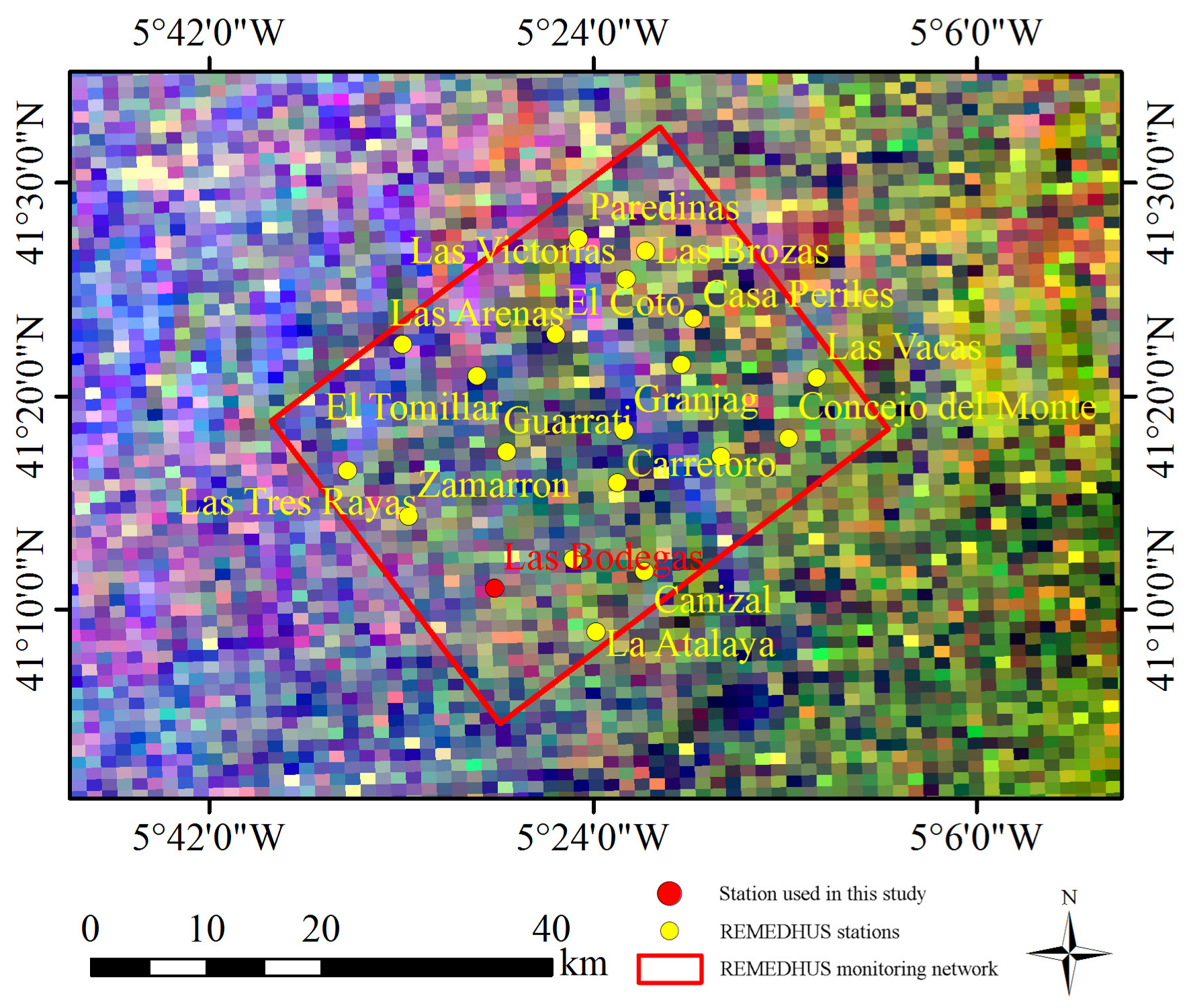
2.1. Study Area

A relatively sparsely vegetated field within the REMEDHUS (REd de MEDiciòn de la HUmedad del Suelo) SM monitoring network (41°8′56″–41°27′21″ N, 5°13′29″–5°35′31″ W) [52] located in the central Douro Basin of Spain was chosen as the study area in this paper. The area of the REMEDHUS is about 1300 km² with altitude ranging from 700 to 900 m. It belongs to the continental semi-arid Mediterranean climate with annual precipitation of 385 mm, potential evaporation of 908 mm, and average temperature of 12 °C. 78% of the vegetation types is the rain-fed cereals, which are generally sowed in autumn, and become mature in early summer.

About 24 ground monitoring stations (Figure 1) were set up from 1999 to 2009, which measure SM and soil temperature at 0–5 cm (Stevens Hydra probe) automatically with a time interval of one hour. As shown in Figure 1, the spatial distribution of in situ sites is uneven. The REMEDHUS network is an important part of the International Soil Moisture Network, and the in situ SM has been widely used to calibrate/validate various satellite SM products. The SM data used in this study are downloaded from the ISMN (https://ismn.geo.tuwien.ac.at, accessed on 8 November 2022). In this study, only the SM data from the station Las Bodegas are selected for the analysis, since this station can represent the typical vegetation and soil surface conditions in the REMEDHUS network [53,54]. Figure 2a displays the in situ SM (blue line) of station Las Bodegas from 1 January 2016 to 31 December 2018 recorded around the imaging time of Sentinel-1A (Section 2.2). The SM generally shows seasonal variations (e.g., deceased in May and increased in August). The topsoil composition includes about 21% clay, 36% sand, and a bulk density of 1.41 g/cm³.

2.2. Sentinel-1A Data and Preprocessing

Three-year Sentinel-1A data ranging from 1 January 2016 to 31 December 2018 with descending orbit are used in this study, which were downloaded from the website of NASA EARTHDATA (https://search.asf.alaska.edu/#/, accessed on 8 November 2022). The reason for only choosing the Sentinel-1A data in the descending orbit is due to the fact that this study only focuses on investigating the changes of effective roughness parameters caused by potential changes of soil surface. In other words, usages of Sentinel-1A data in both descending and ascending orbits or/and from multiple relative orbits may also lead to change of roughness for the same soil surface caused by the variation of incidence angle of Sentinel-1A observations.

Table 1. Information of the Sentinel-1A data.

Parameters	Description
Product type	Ground range detected
Acquisition mode	Interferometric wide swath
Processing level	Level-1
Frequency	5.405 GHz
Polarization mode	VV, VH
Looks for the azimuth and range directions	1 and 5
Grid spacing for the azimuth and range	10 m
Orbit	Descending
Incidence angles	30.56° to 46.42°
Temporal range	1 January 2016–31 December 2018
Temporal resolution	12 days
UTC times	06:25–06:26

lists the specific parameters of the Sentinel-1A data. The preprocessing of the Sentinel-1A data included thermal noise removal, radiometric calibration, speckle filtering, geometric corrections, radiometric normalization, resample (1 km width) and reprojection (datum: UTM WGS84). The Lee sigma method was used to remove the speckle noise of Sentinel-1A data with sigma value of 0.9 and windows size of 7. The Range-Doppler terrain correction was applied to correct the geometric distortion during Sentinel-1A imaging. The bilinear sampling technique was used to resample the Sentinel-1A data into 1 km. Once the preprocessing was complete, the backscatter (in dB) corresponding to the selected station was extracted. According to Bauer-Marschallinger et al. [17], backscatter measurements with very high and very low values are highly unlikely to carry any SM information and thus can be removed. The threshold for the Sentinel-1A VV polarization was restrained within [–20,–5] dB in this study. Figure 2 shows that the Sentinel-1A backscatter (black line) almost follows the dynamic trend of SM (blue line).

2.3. Other Data

In the discussion section, the leaf area index (LAI) was used to parameterize the WCM for quantitatively evaluate the vegetation influence to the results. In this study, the LAI 8-day products obtained from the Terra MODIS were used, which were downloaded from the NASA Goddard Space Flight Center (http://ladsweb.nascom.nasa.gov/data/search.html, accessed on 8 November 2022). The product was projected to WGS 1984 UTM coordinates from the original 1 km SIN Grid data, and the spatial resolution was 1 km. The HANTS filter [55] was employed to smooth the original LAI data in order to suppress the effect of cloud cover. The cubic spline interpolation technique was used on the smoothed LAI data to estimate the LAI values of the dates of Sentinel-1A acquisitions. Figure 2b shows the LAI of station Las Bodegas from 1 January 2016 to 31 December 2018 recorded around the imaging time of Sentinel-1A. It was found that the LAI is generally lower than 1, indicating sparse vegetation condition.

3. Methodology

3.1. Bare Soil Backscattering Modeling

The AIEM was used to simulate the soil backscatter, which is an analytical backscatter model [27,28]. This model can simulate co-polarized backscatter at a given frequency and incidence angle. The autocorrelation function (ACF), correlation length, RMS height, soil dielectric constant (ε), and sensor parameters (wavelength λ and incidence angle θ) are needed to drive the AIEM. The Dobson dielectric mixing model [56] was used to compute the soil dielectric constant from the SM with input of soil texture parameters. The AIEM has been proven to be capable of simulating soil backscatter accurately in relatively wider range of radar configurations and ground conditions [57] than semi-empirical soil models. In general, it is deemed that the validation range is constrained within ks < 3.0 [39], which is suitable for most grassland and agricultural areas without periodical features. The AIEM is conceptually expressed as,

$$\left({\sigma }_{HH}^o,{\sigma }_{VV}^o\right)=AIEM\left(\lambda ,\theta ,\epsilon ,s,l,ACF,sand,cllay,density\right)$$

(1)

where ${\sigma }_{HH}^o$ and ${\sigma }_{VV}^o$ represent the HH- and VV-polarized backscatter and the ACF is characterized by the exponential correlation function. Since the Sentinel-1A provides the VV and VH backscatter and the AIEM can only simulate co-polarized backscatter accurately due to no inclusion of the multiple scattering effects in the model [27,28], the results were limited only to the VV polarization. By comprehensive consideration of the effective range of the AIEM and the sensor configuration of Sentinel-1A, the RMS height was set from 0.1 to 2.6 cm with 0.1 cm interval, and the correlation length varied from 1 to 30 cm with 1.0 cm interval (see

Table 2. Parameters needed for the AIEM.

Satellite configuration	Frequency (f)	5.405 GHz
	Incidence angle (θ)	40°
Surface	SM	In situ measurements
	RMS height (s)	Optimized parameter
	Correlation length (l)	Optimized parameter
	Autocorrelation function	exponentiial
Soil texture	Clay	21%
	Sand	36%
	Bulk density	1.41 g/cm3

). The reason to set these ranges was to fulfil the valid range of applying the AIEM. The exponential autocorrelation function was adopted in this study due to the fact that this function has mostly been applied to sparse vegetation condition [14,58,59].

3.2. Backscatter Simulation and SM Retrieval Based on AIEM

The AIEM was used to test the assumption on the constant effective roughness parameters from the perspective of backscatter simulation and SM retrieval from Sentinel-1A data over a sparsely vegetated field. In this study, the effect of vegetation was ignored due to the fact that the vegetation coverage is sparse (see Section 2.3). The validity of this assumption is further discussed in Section 5.2. The procedures for selecting the effective roughness parameters, simulating backscatter, and retrieving SM are listed in the following steps.

Step 1: Sentinel-1A data grouping. Three-year Sentinel-1A data were separated as six different temporal periods, that is “2016”, “2017”, ”2018”, ”2016 + 2017”, ”2017 + 2018”, and ”2016 + 2017 + 2018”, to compute the effective roughness parameters at different temporal scales. For example, the “2016” stands for the parameters of effective roughness optimized based on the Sentinel-1A observations acquired in 2016 and “2017 + 2018” represents the optimized roughness parameters computed from the Sentinel-1A data acquired in 2017 and 2018.

Step 2: Estimation of soil scattering. The VV-polarized backscatter of bare soil was simulated by the AIEM. The frequency (5.405 GHz) and incidence angle (40°) were referred to the sensor configuration of Sentinel-1A (Table 1). The RMS height varies from 0.1 to 2.6 cm with an interval of 0.1 cm and the correlation length varied from 1 to 30 cm with an interval of 1 cm. The Dobson dielectric mixing model [56] was used to compute the soil dielectric constant from the in situ SM measured in 2016 with input of soil texture.

Step 3: Computation of root mean square error (RMSE) matrix. The RMSE between Sentinel-1A observation and AIEM simulation (RMSES1-AIEM) was computed for each pair of RMS height and correlation length. The size of the RMSES1-AIEM matrix is 26 × 30.

$$RMS{E}_{S1\_AIEM}=\sqrt{\frac{1}{n}}{{\displaystyle \sum }}_{i=1}^n{\left({\sigma }_{S1A,i}^o-{\sigma }_{AIEM,i}^o\right)}^2$$

(2)

Step 4: Selection of effective roughness parameters. There were two restrictions on the selection of effective roughness parameters. On one hand, the ratio between RMS height and correlation length should be less than 0.086, which ensured the effective roughness parameters below the diagonal line. Under this premise satisfied, the pair of RMS height and correlation length making the values of RMSES1-AIEM to its minimum were considered as the final effective roughness parameters in “2016”.

$${\left\{s,l\right\}}_{effective}=\{\begin{array}{c}s/l<0.086\\ min\left\{RMS{E}_{S1\_AIEM}\right\}\end{array}$$

(3)

Step 5: Steps 2–4 were repeated with the other temporal periods of Sentinel-1A data, “2017”, “2018”, “2016 + 2017”, “2017 + 2018”, and “2016 + 2017 + 2018”. This means the effective roughness parameters were selected for each temporal period.

Step 6: Backscatter simulation. With the effective roughness parameters selected at different temporal periods, the AIEM was implemented to simulate the backscatter from 2016 to 2018. The input parameters of the AIEM were the same under different simulation cases, and only the roughness parameters were different.

Step 7: SM retrieval. Based on the AIEM implemented with optimized effective roughness parameters, we used a look-up-table (LUT) method to retrieve SM from Sentinel-1A data. The LUT was built using calibrated AIEM with SM ranging from 0.01 m³/m³ to 0.35 m³/m³ with 0.01 m³/m³ interval. The maximum value of SM referred to the dynamic range of in situ SM. The cost function C is written in Equation (4). The SM corresponding to the minimum S was considered as the retrieved SM.

$$\mathrm{C}=\min \left\{{\left({\sigma }_{S1A,i}^o-{\sigma }_{AIEM,i}^o\right)}^2\right\}$$

(4)

3.3. Change Detection Method for SM Retrieval

The TU Wien Change Detection Model [60] was adopted for Sentinel-1 SM retrieval, which interprets the changes of backscatter as changes in SM, and the vegetation structure and surface roughness are treated as static parameters. This method was established based on relatively long time series backscatter data. For the SM estimation, the Sentinel-1A observation at time t and observation angle (θ) were normalized to a reference angle (Θ) and linearly scaled between wet and dry reference values,

$$\mathrm{SSM}\left(\mathrm{t}\right)=\frac{\Delta {\sigma }^o\left(\mathsf{\Theta },t\right)}{{\sigma }_{wet}^o\left(\mathsf{\Theta }\right)-{\sigma }_{dry}^o\left(\mathsf{\Theta }\right)}$$

(5)

where $\Delta {\sigma }^o\left(\mathsf{\Theta },t\right)$ is the change in normalized backscatter (relative to dry conditions). It is worth pointing out that the SM estimation from (5) is not the volumetric SM but the relative surface soil water saturation, and it is written as SSM. The reference angle was chosen as 40° as it is close to the center location in the range of local incidence angle in Sentinel-1A observations [17]. The above Equation (5) can be re-written as,

$$\mathrm{SSM}\left(\mathrm{t}\right)=\frac{{\sigma }^o\left(40,t\right)-{\sigma }_{dry}^o\left(40\right)}{{\sigma }_{wet}^o\left(40\right)-{\sigma }_{dry}^o\left(40\right)} [\%]$$

(6)

In (6), the backscatter values were normalized to the reference 40° as follows,

$${\sigma }^o\left(40,t\right)={\sigma }^o\left(40,t\right)-{\beta }_r\left(\theta -40°\right)\left[dB\right]$$

(7)

$${\beta }_r=aS+b\overline{{\sigma }^o}+c \left[dB/°\right]$$

(8)

where S stands for the sensitivity ($\mathrm{S}={\sigma }_{wet}^o\left(40\right)-{\sigma }_{dry}^o\left(40\right)$), $\overline{{\sigma }^o}$ is the mean backscatter for the selected study period. The coefficients were constant as [17],

$$\left[\begin{array}{c}a\\ b\\ c\end{array}\right]=\left[\begin{array}{c}-0.01725\\ 0.00553\\ 0.02546\end{array}\right]$$

(9)

For each grid point, the dry and wet reference backscattering coefficients were estimated through the 10% and 90% of the normalized backscatter time series as,

$${\sigma }_{dry}^o\left(40\right)=\frac{0\%-d}{k} \left[dB\right]$$

(10)

$${\sigma }_{wet}^o\left(40\right)=\frac{100\%-d}{k} \left[dB\right]$$

(11)

$$k=\frac{90\%-10\%}{{\sigma }_{P_{90}}^o\left(40\right)-{\sigma }_{P_{10}}^o\left(40\right)}$$

(12)

$$d=90\%-k{\sigma }_{P_{90}}^o\left(40\right)$$

(13)

Finally, the relative soil moisture SSM was transferred to the volumetric soil moisture based on the minimum and maximum values of the in situ measurements.

$$SM=SSM\times \left[max\left(S{M}_{in-situ}\right)-min\left(S{M}_{in-situ}\right)\right]+min\left(S{M}_{in-situ}\right)$$

(14)

3.4. Accuracy Evaluation

The following errors metrics, i.e., Bias, RMSE, ubRMSE, and R, were adopted to assess the accuracy of backscatter simulation and SM retrieval.

$$\mathrm{Bias}=\frac{1}{n}\left({{\displaystyle \sum }}_{i=1}^n{V}_{est}-{{\displaystyle \sum }}_{i=1}^n{V}_{obs}\right)$$

(15)

$$\mathrm{RMSE}=\sqrt{\frac{1}{n}{{\displaystyle \sum }}_{i=1}^n{\left(V_{est}-V_{obs}\right)}^2}$$

(16)

$$\mathrm{ubRMSE}=\sqrt{RMS{E}^2-Bia{s}^2}$$

(17)

$$\mathrm{R}=\frac{{{\displaystyle \sum }}_{i=1}^n\left(V_{est}-\overline{V_{est}}\right)\left(V_{obs}-\overline{V_{obs}}\right)}{\sqrt{{{\displaystyle \sum }}_{i=1}^n{\left(V_{est}-\overline{V_{est}}\right)}^2}\sqrt{{{\displaystyle \sum }}_{i=1}^n{\left(V_{obs}-\overline{V_{obs}}\right)}^2}}$$

(18)

where $V_{obs}$ indicates the Sentinel-1A backscatter or the in situ SM, $V_{est}$ indicates the AIEM simulation or the retrieved SM, $\overline{V_{obs}}$ and $\overline{V_{est}}$ are their average values, and n is the number of sample data.

4. Results

4.1. Effective Roughness Parameters

The effective roughness parameters are selected during different temporal periods complying with the two restrictions in Equation (3). Figure 3 displays the distribution of the RMSE_{S1_AIEM} between the Sentinel-1A observation and AIEM simulation along the directions of RMS height and correlation length at different temporal periods. Figure 4 displays all the optimized parameters at different temporal periods.

Table 3. Effective roughness parameters optimized at different temporal periods.

Period of Calibration Datasets	Effective Roughness
	RMS Height (cm)	Correlation Length (cm)
2016	1.3	30
2017	1.3	28
2018	1.2	27
2016 + 2017	1.3	29
2017 + 2018	1.3	30
2016 + 2017 + 2018	1.3	30

lists the final selected effective roughness parameters.

Figure 3 shows that the distributions and changing trends of the RMSE_{S1_AIEM} computed at different temporal periods are similar. As RMS height and correlation length increase, the RMSE_{S1_AIEM} decreases first and increases later on. This indicates that the optimized values for the RMS height and correlation length are located at the inflection points. In addition, it is noticed that there are some contours distributed in the RMSE_{S1_AIEM}. On one hand, the combination of RMS height and correlation length on the contours can achieve the same RMSE_{S1_AIEM}, which means there are multiple solutions. On the other hand, the combination of RMS height and correlation length on the contours verifies that the impact of increased RMS height caused to the RMSE_{S1_AIEM} can be balanced by increased correlation length. Taking into account the interaction between the RMS height and correlation length, only the combinations of RMS height and correlation length below the diagonal line (Figure 4) are considered as the possible optimization results. The changes of the RMSE_{S1_AIEM} located outside the defined range are not discussed here.

From Figure 4, it can be seen that the possible effective roughness parameters (corresponding to the five smallest RMSE_{S1_AIEM} are distributed into two different sub-spaces, which is divided by diagonal, which can also be found in Figure 3. Only the sub-space below the diagonal is considered as the possible optimization results. It is interesting that the optimized possible roughness parameters gather together. The minimum and maximum of optimized RMS height are 0.9 to 1.3 cm, and the optimized correlation length varies from 14 to 30 cm. Table 3 lists the final effective roughness parameters optimized at different temporal periods, which are very close to each other (circles with red edge). The optimized value of RMS height equals 1.3 cm except in 2018 (1.2 cm) and the correlation length ranges from 27 to 30 cm. It can be said that the effective roughness parameters optimized at different temporal periods tends to be consistent. Though the roughness parameters may be changed at adjacent acquisitions due to tillage practices or heavy rainfall event in agricultural fields [47,48,49], the effective roughness parameters tend to be consistent on an annual scale.

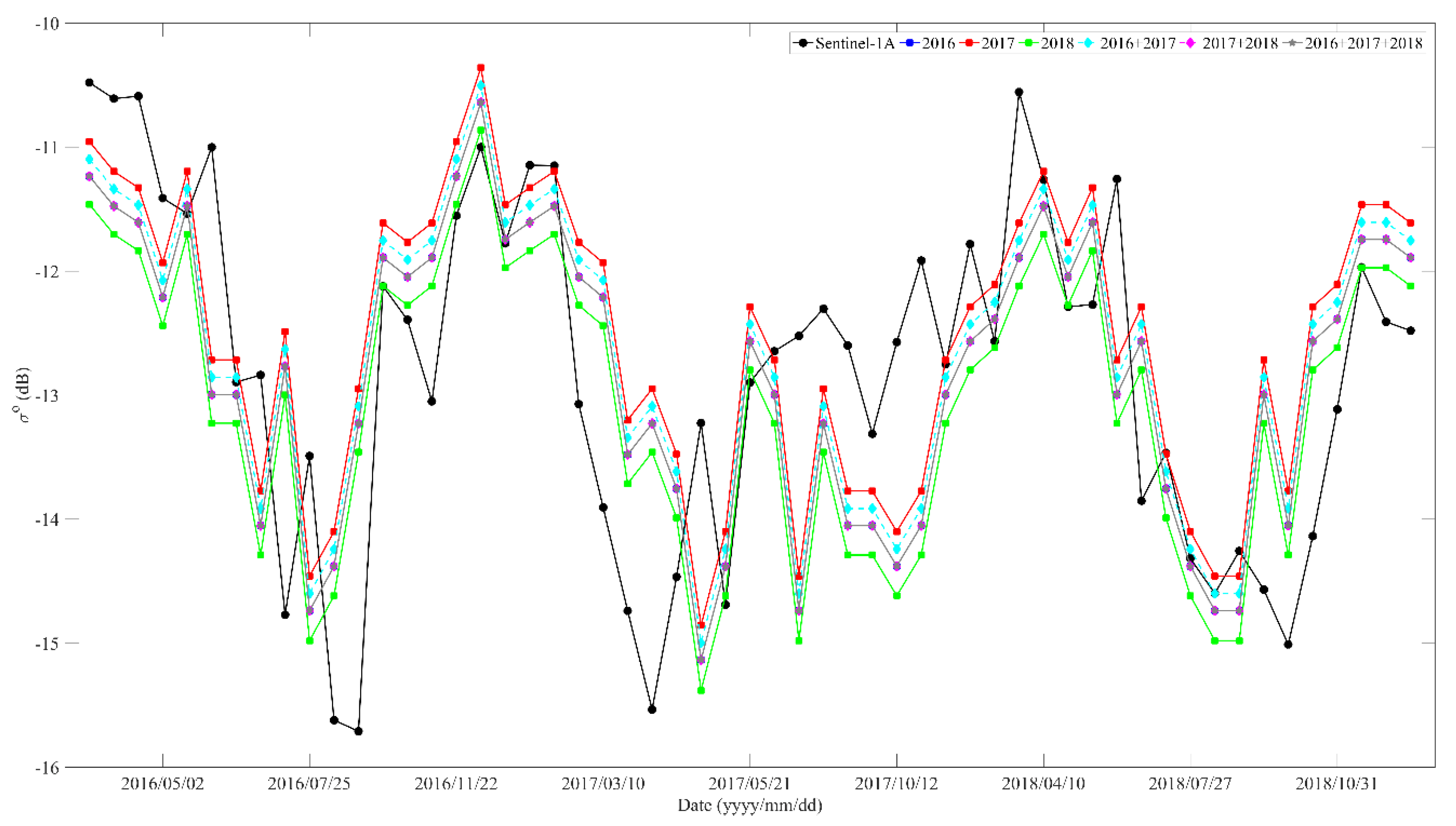
4.2. Backscatter Simulation Results

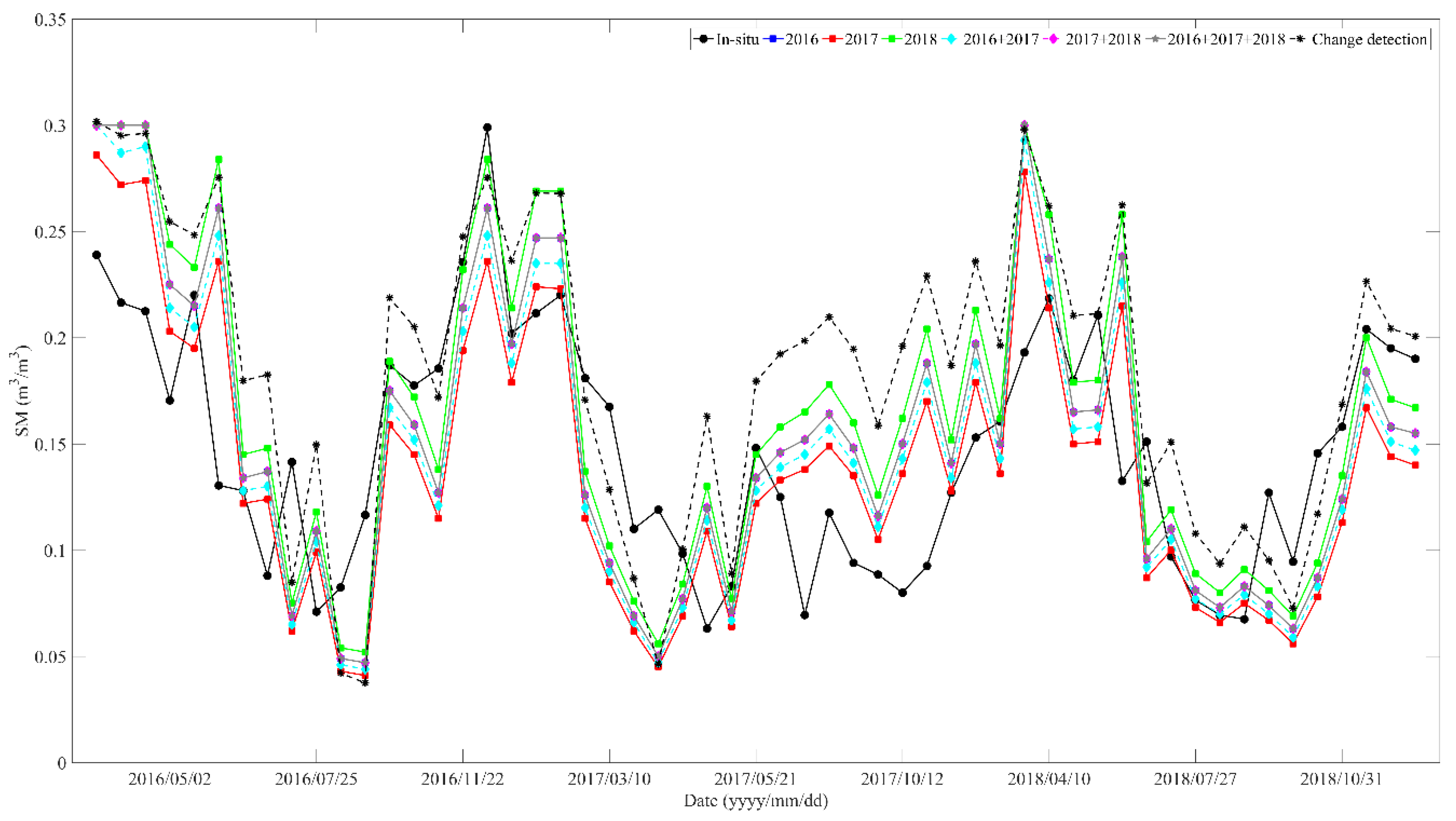
The AIEM in combination with the selected effective roughness parameters was implemented to simulate the VV-polarized backscatter with in situ SM from 1 January 2016 to 31 December 2018.

Table 4. Evaluation metrics between the Sentinel-1A backscatter and AIEM simulation.

Period of Calibration Datasets	Bias (dB)	RMSE (dB)	RMSE (dB)	R (-)
2016	−0.019	1.133	1.133	0.616
2017	0.260	1.163	1.133	0.616
2018	−0.252	1.162	1.135	0.616
2016 + 2017	−0.118	1.139	1.133	0.616
2017 + 2018	−0.019	1.133	1.133	0.616
2016 + 2017 + 2018	−0.019	1.133	1.133	0.616

presents the evaluation metrics between the Sentinel-1A observation and AIEM simulation. The statistical indicators illustrate that the simulated backscatter with different combinations of effective roughness parameters was almost the same with R values all equal to 0.616 and RMSE ranging from 1.133 to 1.163 dB. The Bias values indicate the simulated backscatter was overestimated with effective roughness parameters computed in 2017 and 2016 + 2017 and underestimated in 2016, 2018, 2017 + 2018, and 2016 + 2017 + 2018. Analyzed by the evaluation metrics, the effective roughness parameters computed at different temporal periods achieved similar simulation results.

Figure 5 displays the Sentinel-1A observation and AIEM simulation with different effective roughness parameters acquired at different temporal periods. The plots show that the backscatter simulated by the calibrated AIEM generally captures well the dynamics of Sentinel-1A observation. The influences of RMS height and correlation length on the backscatter simulation have also been distinguished. The RMS height equals 1.2 cm when the Sentinel-1A data in 2018 are used, which is slightly lower than others (1.3 cm). This leads to the lower simulated backscatter (green line in Figure 5). With the increase of optimized correlation length, the simulated backscatter decreases. Nevertheless, there is little difference between the simulated backscatter with different optimized RMS height and correlation length, which is also reflected in the evaluation metric (Table 4). The computed Bias, RMSE, and R are very close to each other for the six cases. These results validate that assumption of the constant of effective roughness parameters is reasonable, which can be adopted for parameterizing the roughness in the AIEM for backscatter simulation at least in three years. It should be noted that the simulated backscatter for 2017 seems to have much larger error than the other 2 years using various effectiveness roughness, which is mainly due to the fact that the in situ SM does not well represent the actual condition of satellite scale.

4.3. SM Retrieval

The SM was directly retrieved from Sentinel-1A data from 1 January 2016 to 31 December 2018 using the established LUT with the calibrated AIEM.

Table 5. Statistical errors computed between the in situ measurement and SM retrievals.

Retrieval Method	Period of Calibration Datasets	Bias (m3/m3)	RMSE (m3/m3)	RMSE (m3/m3)	R (-)
AIEM	2016	0.006	0.052	0.052	0.685
	2017	−0.008	0.049	0.049	0.684
	2018	0.017	0.056	0.053	0.689
	2016 + 2017	−0.001	0.050	0.050	0.684
	2017 + 2018	0.006	0.052	0.052	0.685
	2016 + 2017 + 2018	0.006	0.052	0.052	0.685
Change detection	2016 + 2017 + 2018	0.036	0.065	0.054	0.658

presents the statistical errors computed between the in situ data and SM retrievals. It can be found that there are few differences noted between different effective roughness parameters with R values floating at 0.685 and RMSEs ranging from 0.049 to 0.052 m³/m³. Overall, the error metrics obtained with the calibrated AIEM are comparable with the results recently reported for SAR-based SM retrievals. For example, Ma et al. [19] combined Sentinel-1 and Sentinel-2 for retrieving SM with RMSE ranging between 0.039 m³/m³ and 0.078 m³/m³. Bai et al. [18] obtained the SM retrievals from Sentinel-1A data with RMSE varying from 0.076 m³/m³ to 0.103 m³/m³. In addition, the evaluation metrics show this method achieved better performance for SM retrieval than the change detection method. It is concluded that the accuracy of retrieved SM is in line with the state-of-the-art retrieval results from Sentinel-1 data.

Figure 6 presents the in situ and retrieved SM based on calibrated AIEM with different effective roughness parameters and the retrieval results of the change detection method. The plots illustrate that the retrieved SM captures well the seasonal dynamics of in situ SM. The SM decreases from spring to the later summer and then increases toward to the winter. The retrieved SM measurements using different effective roughness parameters are very close to each other, and their amplitude and dynamic change are very similar. However, it is worth pointing out that the retrieved SM is overestimated on some dates. This also confirmed the possible change of roughness parameters at adjacent acquisition of Sentinel-1A, which is not against with the assumption on the effective roughness parameters. The dynamics of SM retrieved from change detection method almost follow the change of the ones from the AIEM, while some values are overestimated. From the dynamics analysis and statistical indicators, it is concluded that the effective roughness parameters can be used for parameterizing the AIEM and then used for SM retrieval from Sentinel-1A data at least three years over sparsely vegetated fields.

5. Discussion

5.1. Comparison between Optimized and Effective Values

During the process of searching for optimization roughness parameters, the RMS height and correlation length located above the diagonal are ignored. For example, the best results optimized for 2017 are 1.7 and 2.0 cm for RMS height and correlation length, respectively, and the selected effective parameters are 1.3 cm and 28 cm for RMS height and correlation length, which is the second-best result. For another example, the best results optimized for 2016 + 2017 are 2.6 cm and 5.0 cm for RMS height and correlation length and the selected effective parameters are 1.3 cm and 29 cm for RMS height and correlation length, which is the second-best result, respectively. The statistical metric between the Sentinel-1A backscatter and AIEM simulation with the best optimization parameters are listed in

Table 6. Statistical metric between Sentinel-1A observation (in situ SM) and AIEM simulation (retrieved SM) with the best optimization parameters.

Period of Calibration Datasets	Backscatter Simulation				SM Retrieval
	Bias (dB)	RMSE (dB)	RMSE (dB)	R (-)	Bias (m3/m3)	RMSE (m3/m3)	RMSE (m3/m3)	R (-)
2017	−0.200	1.149	1.132	0.616	0.005	0.050	0.050	0.683
2016 + 2017	−0.152	1.142	1.132	0.616	0.002	0.050	0.050	0.683

. It is found that the results of backscatter simulation and SM achieved from the effective roughness parameters are almost the same as the results achieved with the best optimization parameters. This proves the rationality of the constraint condition on the selection of effective roughness parameters.

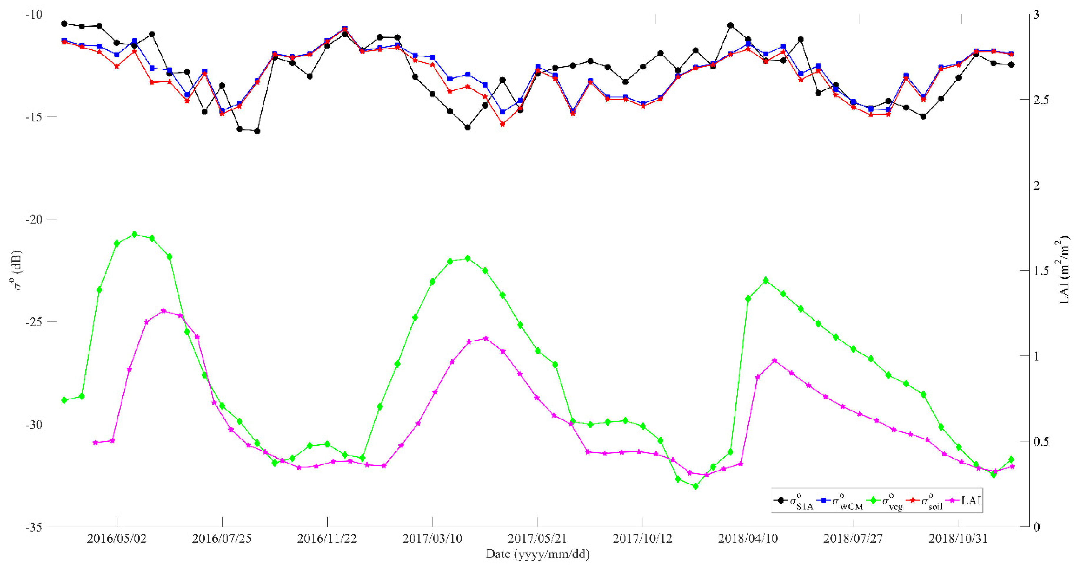
5.2. Vegetation Effect

The assumption on the effective roughness parameters was tested over a sparsely vegetated field in this study, and the impact of vegetation was ignored. To further test whether the assumption is valid, the AIEM was coupled with the WCM to investigate the contributions of soil and vegetation scattering following previous works [18,46]. The effective roughness parameters computed at “2016 + 2017 + 2018” were used as the parameter values of AIEM, and the coefficients A and B of WCM are optimized using the least square method. The vegetation parameter needed for parameterizing the vegetation scattering and attenuation in WCM was characterized by the LAI (Section 2.3). A detailed description of the LAI can be seen in Han et al. [46]. Using the Sentinel-1A data acquired from 2016 to 2018, the computed coefficients A and B were 0.1109 and 0.0248, respectively.

Figure 7 displays the Sentinel-1A backscatter and WCM simulation from 2016 to 2018. It was found that the vegetation contribution complies with the trend of LAI. The maximum vegetation contribution occurs in May and June, and the minimum occurs in November and December. The soil contribution is much larger and higher than the vegetation contribution, which is very close to the total simulate backscatter of WCM. This confirms that the vegetation contribution can be ignored during the study period, even in the peak growth of vegetation.

6. Conclusions

In this study, the AIEM is used to test the assumption on the constant effective roughness parameters for parameterizing the surface roughness. Three years of Sentinel-1A data acquired in the REMEDHUS SM network is used. To evaluate the temporal dynamic of the effective roughness parameters, the effective roughness parameters are computed at different temporal periods, including 2016, 2017, 2018, 2016 + 2017, 2017 + 2018, and 2016 + 2017 + 2018. During each temporal period, the roughness parameters are assumed to be unchanged. The RMSE between Sentinel-1A observation and AIEM simulation are minimized to find the effective roughness parameters. Once the effective roughness parameters are determined, they will be used as input of the AIEM for simulating Sentinel-1A backscatter and retrieving SM from 1 January 2016 to 31 December 2018. The Sentinel-1A observation is reproduced well by using the calibrated AIEM. In addition, the retrieved SM is in line with the in situ measurement, and the seasonal trend of SM is well captured. The effective roughness parameters method achieved better performance for SM retrieval than the change detection method. The differences between backscatter simulation and SM retrieval caused by the optimized and effective values have been carefully discussed, which further validate the feasibility of the effective roughness parameters for describing the surface conditions. In conclusion, the investigations show that the assumption regarding the constant effective roughness parameters is reasonable, and this method can be used for helping backscatter simulation and SM retrieval. It should be noted that only one station of REMEDHUS network was used for the analysis given the fact that this station can represent the typical vegetation and soil surface conditions in this area, while other stations can also be implemented to confirm the finding drawn upon in this study in the future work. In addition, further studies should be undertaken to validate this method on different land covers in longer time series by combining Sentinel-1A and Sentinel-1B data.

References

1. Kornelsen, K.C.; Coulibaly, P. Advances in soil moisture retrieval from synthetic aperture radar and hydrological applications. J. Hydrol. 2013, 476, 460–489. [Google Scholar] [CrossRef]
2. Seneviratne, S.I.; Corti, T.; Davin, E.L.; Hirschi, M.; Jaeger, E.B.; Lehner, I.; Orlowsky, B.; Teuling, A.J. Investigating soil moisture–climate interactions in a changing climate: A review. Earth-Sci. Rev. 2010, 99, 125–161. [Google Scholar] [CrossRef]
3. Zheng, D.; Van der Velde, R.; Su, Z.; Wang, X.; Wen, J.; Booij, M.J.; Hoekstra, A.Y.; Chen, Y. Augmentations to the Noah Model Physics for Application to the Yellow River Source Area. Part I: Soil Water Flow. J. Hydrometeorol. 2015, 16, 2659–2676. [Google Scholar] [CrossRef]
4. Sutanudjaja, E.H.; van Beek, L.P.H.; de Jong, S.M.; van Geer, F.C.; Bierkens, M.F.P. Calibrating a large-extent high-resolution coupled groundwater-land surface model using soil moisture and discharge data. Water Resour. Res. 2014, 50, 687–705. [Google Scholar] [CrossRef]
5. He, B.; Xing, M.; Bai, X. A Synergistic Methodology for Soil Moisture Estimation in an Alpine Prairie Using Radar and Optical Satellite Data. Remote Sens. 2014, 6, 10966–10985. [Google Scholar] [CrossRef] [Green Version]
6. Zheng, D.; van der Velde, R.; Su, Z.; Wen, J.; Wang, X.; Yang, K. Impact of soil freeze-thaw mechanism on the runoff dynamics of two Tibetan rivers. J. Hydrol. 2018, 563, 382–394. [Google Scholar] [CrossRef]
7. Moran, M.S.; Inoue, Y.; Barnes, E. Opportunities and limitations for image-based remote sensing in precision crop management. Remote Sens. Environ. 1997, 61, 319–346. [Google Scholar] [CrossRef]
8. Dorigo, W.A.; Xaver, A.; Vreugdenhil, M.; Gruber, A.; Hegyiová, A.; Sanchis-Dufau, A.D.; Zamojski, D.; Cordes, C.; Wagner, W.; Drusch, M. Global Automated Quality Control of In Situ Soil Moisture Data from the International Soil Moisture Network. Vadose Zone J. 2013, 12, 1–21. [Google Scholar] [CrossRef]
9. Walker, J.P.; Willgoose, G.R.; Kalma, J.D. In situ measurement of soil moisture: A comparison of techniques. J. Hydrol. 2004, 293, 85–99. [Google Scholar] [CrossRef]
10. Zhang, P.; Zheng, D.; van der Velde, R.; Wen, J.; Zeng, Y.; Wang, X.; Wang, Z.; Chen, J.; Su, Z. Status of the Tibetan Plateau observatory (Tibet-Obs) and a 10-year (2009–2019) surface soil moisture dataset. Earth Syst. Sci. Data 2021, 13, 3075–3102. [Google Scholar] [CrossRef]
11. Petropoulos, G.P.; Ireland, G.; Barrett, B. Surface soil moisture retrievals from remote sensing: Current status, products & future trends. Phys. Chem. Earth Parts A/B/C 2015, 83–84, 36–56. [Google Scholar] [CrossRef]
12. Zheng, D.; Wang, X.; van der Velde, R.; Ferrazzoli, P.; Wen, J.; Wang, Z.; Schwank, M.; Colliander, A.; Bindlish, R.; Su, Z. Impact of surface roughness, vegetation opacity and soil permittivity on L-band microwave emission and soil moisture retrieval in the third pole environment. Remote Sens. Environ. 2018, 209, 633–647. [Google Scholar] [CrossRef]
13. Karthikeyan, L.; Pan, M.; Wanders, N.; Kumar, D.N.; Wood, E.F. Four decades of microwave satellite soil moisture observations: Part 1. A review of retrieval algorithms. Adv. Water Resour. 2017, 109, 106–120. [Google Scholar] [CrossRef]
14. Zheng, D.; Li, X.; Wen, J.; Hofste, J.G.; van der Velde, R.; Wang, X.; Wang, Z.; Bai, X.; Schwank, M.; Su, Z. Active and Passive Microwave Signatures of Diurnal Soil Freeze-Thaw Transitions on the Tibetan Plateau. IEEE Trans. Geosci. Remote Sens. 2021, 60, 4301814. [Google Scholar] [CrossRef]
15. Barrett, B.; Dwyer, E.; Whelan, P. Soil Moisture Retrieval from Active Spaceborne Microwave Observations: An Evaluation of Current Techniques. Remote Sens. 2009, 1, 210–242. [Google Scholar] [CrossRef] [Green Version]
16. Paloscia, S.; Pettinato, S.; Santi, E.; Notarnicola, C.; Pasolli, L.; Reppucci, A. Soil moisture mapping using Sentinel-1 images: Algorithm and preliminary validation. Remote Sens. Environ. 2013, 134, 234–248. [Google Scholar] [CrossRef]
17. Bauer-Marschallinger, B.; Freeman, V.; Cao, S.; Paulik, C.; Schaufler, S.; Stachl, T.; Modanesi, S.; Massari, C.; Ciabatta, L.; Brocca, L.; et al. Toward Global Soil Moisture Monitoring with Sentinel-1: Harnessing Assets and Overcoming Obstacles. IEEE Trans. Geosci. Remote Sens. 2019, 57, 520–539. [Google Scholar] [CrossRef]
18. Bai, X.; He, B.; Li, X.; Zeng, J.; Wang, X.; Wang, Z.; Zeng, Y.; Su, Z. First Assessment of Sentinel-1A Data for Surface Soil Moisture Estimations Using a Coupled Water Cloud Model and Advanced Integral Equation Model over the Tibetan Plateau. Remote Sens. 2017, 9, 714. [Google Scholar] [CrossRef] [Green Version]
19. Ma, C.; Li, X.; McCabe, M.F. Retrieval of High-Resolution Soil Moisture through Combination of Sentinel-1 and Sentinel-2 Data. Remote Sens. 2020, 12, 2303. [Google Scholar] [CrossRef]
20. Ezzahar, J.; Ouaadi, N.; Zribi, M.; Elfarkh, J.; Aouade, G.; Khabba, S.; Er-Raki, S.; Chehbouni, A.; Jarlan, L. Evaluation of Backscattering Models and Support Vector Machine for the Retrieval of Bare Soil Moisture from Sentinel-1 Data. Remote Sens. 2019, 12, 72. [Google Scholar] [CrossRef]
21. Balenzano, A.; Mattia, F.; Satalino, G.; Lovergine, F.P.; Palmisano, D.; Peng, J.; Marzahn, P.; Wegmüller, U.; Cartus, O.; Dąbrowska-Zielińska, K.; et al. Sentinel-1 soil moisture at 1 km resolution: A validation study. Remote Sens. Environ. 2021, 263, 112554. [Google Scholar] [CrossRef]
22. Oh, Y.; Sarabandi, K.; Ulaby, F.T. An empirical model and an inversion technique for radar scattering from bare soil surfaces. IEEE Trans. Geosci. Remote Sens. 1992, 30, 370–381. [Google Scholar] [CrossRef]
23. Oh, Y.; Sarabandi, K.; Ulaby, F.T. Semi-Empirical Model of the Ensemble-Averaged Differential Mueller Matrix for Microwave Backscattering from Bare Soil Surfaces. IEEE Trans. Geosci. Remote Sens. 2002, 40, 1348–1355. [Google Scholar] [CrossRef] [Green Version]
24. Oh, Y. Quantitative Retrieval of Soil Moisture Content and Surface Roughness from Multipolarized Radar Observations of Bare Soil Surfaces. IEEE Trans. Geosci. Remote Sens. 2004, 42, 596–601. [Google Scholar] [CrossRef]
25. Dubois, P.C.; van Zyl, J.; Engman, T. Measuring soil moisture with imaging radars. IEEE Trans. Geosci. Remote Sens. 1995, 33, 915–926. [Google Scholar] [CrossRef] [Green Version]
26. Fung, A.K. Microwave Scattering and Emission Models and Their Applications; Artech House Publishers: Norwell, MA, USA, 1994. [Google Scholar]
27. Wu, T.D.; Chen, K.S.; Shi, J.C.; Fung, A.K. A transition model for the reflection coefficients in surface scattering. IEEE Trans. Geosci. Remote Sens. 2001, 39, 2040–2050. [Google Scholar]
28. Chen, K.S.; Tzong-Dar, W.; Leung, T.; Qin, L.; Jiancheng, S.; Fung, A.K. Emission of rough surfaces calculated by the integral equation method with comparison to three-dimensional moment method simulations. IEEE Trans. Geosci. Remote Sens. 2003, 41, 90–101. [Google Scholar] [CrossRef]
29. Ulaby, F.T.; Sarabandi, K.; McDonald, K.; Whitt, M.; Dobson, M.C. Michigan microwave canopy scattering model. Int. J. Remote Sens. 1990, 11, 1223–1253. [Google Scholar] [CrossRef]
30. Bracaglia, M.; Ferrazzoli, P.; Guerriero, L. A fully polarimetric multiple scattering model for crops. Remote Sens. Environ. 1995, 54, 170–179. [Google Scholar] [CrossRef]
31. Ferrazzoli, P.; Guerriero, L. Passive microwave remote sensing of forests: A model investigation. IEEE Trans. Geosci. Remote Sens. 1996, 34, 433–443. [Google Scholar] [CrossRef]
32. Zheng, D.; Wang, X.; van der Velde, R.; Zeng, Y.; Wen, J.; Wang, Z.; Schwank, M.; Ferrazzoli, P.; Su, Z. L-Band Microwave Emission of Soil Freezesc-Thaw Process in the Third Pole Environment. IEEE Trans. Geosci. Remote Sens. 2017, 55, 5324–5338. [Google Scholar] [CrossRef]
33. Zheng, D.; Li, X.; Zhao, T.; Wen, J.; Velde, R.V.D.; Schwank, M.; Wang, X.; Wang, Z.; Su, Z. Impact of Soil Permittivity and Temperature Profile on L-Band Microwave Emission of Frozen Soil. IEEE Trans. Geosci. Remote Sens. 2020, 59, 4080–4093. [Google Scholar] [CrossRef]
34. Joseph, A.T.; van der Velde, R.; O‘Neill, P.E.; Lang, R.H.; Gish, T. Soil Moisture Retrieval during a Corn Growth Cycle Using L-Band (1.6 GHz) Radar Observations. IEEE Trans. Geosci. Remote Sens. 2008, 46, 2365–2374. [Google Scholar] [CrossRef] [Green Version]
35. Joseph, A.T.; van der Velde, R.; O‘Neill, P.E.; Lang, R.; Gish, T. Effects of corn on C- and L-band radar backscatter: A correction method for soil moisture retrieval. Remote Sens. Environ. 2010, 114, 2417–2430. [Google Scholar] [CrossRef]
36. Attema, E.P.W.; Ulaby, F.T. Vegetation modeled as a water cloud. Radio Sci. 1978, 13, 357–364. [Google Scholar] [CrossRef]
37. Bai, X.; He, B.; Xing, M.; Li, X. Method for soil moisture retrieval in arid prairie using TerraSAR-X data. J. Appl. Remote Sens. 2015, 9, 096062. [Google Scholar] [CrossRef]
38. Lievens, H.; Verhoest, N.E.C.; De Keyser, E.; Vernieuwe, H.; Matgen, P.; Álvarez-Mozos, J.; De Baets, B. Effective roughness modelling as a tool for soil moisture retrieval from C- and L-band SAR. Hydrol. Earth Syst. Sci. 2011, 15, 151–162. [Google Scholar] [CrossRef] [Green Version]
39. Lievens, H.; Verhoest, N.E.C. On the Retrieval of Soil Moisture in Wheat Fields from L-Band SAR Based on Water Cloud Modeling, the IEM, and Effective Roughness Parameters. IEEE Geosci. Remote Sens. Lett. 2011, 8, 740–744. [Google Scholar] [CrossRef]
40. Bai, X.; He, B. Potential of Dubois model for soil moisture retrieval in prairie areas using SAR and optical data. Int. J. Remote Sens. 2015, 36, 5737–5753. [Google Scholar] [CrossRef]
41. Zhu, L.; Walker, J.P.; Tsang, L.; Huang, H.; Ye, N.; Rüdiger, C. A multi-frequency framework for soil moisture retrieval from time series radar data. Remote Sens. Environ. 2019, 235, 111433. [Google Scholar] [CrossRef]
42. Zhu, L.; Walker, J.P.; Shen, X. Stochastic ensemble methods for multi-SAR-mission soil moisture retrieval. Remote Sens. Environ. 2020, 251, 112099. [Google Scholar] [CrossRef]
43. Zhu, L.; Walker, J.P.; Tsang, L.; Huang, H.; Ye, N.; Rüdiger, C. Soil moisture retrieval from time series multi-angular radar data using a dry down constraint. Remote Sens. Environ. 2019, 231, 111237. [Google Scholar] [CrossRef]
44. Zribi, M.; Dechambre, M. A new empirical model to retrieve soil moisture and roughness from C-band radar data. Remote Sens. Environ. 2002, 84, 42–52. [Google Scholar] [CrossRef]
45. Su, Z.; Troch, P.A.; De Troch, F.P. Remote sensing of bare surface soil moisture using EMAC/ESAR data. Int. J. Remote Sens. 1997, 18, 2105–2124. [Google Scholar] [CrossRef]
46. Han, Y.; Bai, X.; Shao, W.; Wang, J. Retrieval of Soil Moisture by Integrating Sentinel-1A and MODIS Data over Agricultural Fields. Water 2020, 12, 1726. [Google Scholar] [CrossRef]
47. Baghdadi, N.; King, C.; Chanzy, A.; Wigneron, J.P. An empirical calibration of the integral equation model based on SAR data, soil moisture and surface roughness measurement over bare soils. Int. J. Remote Sens. 2002, 23, 4325–4340. [Google Scholar] [CrossRef]
48. Baghdadi, N.; Gherboudj, I.; Zribi, M.; Sahebi, M.; King, C.; Bonn, F. Semi-empirical calibration of the IEM backscattering model using radar images and moisture and roughness field measurements. Int. J. Remote Sens. 2004, 25, 3593–3623. [Google Scholar] [CrossRef]
49. Baghdadi, N.; Holah, N.; Zribi, M. Calibration of the Integral Equation Model for SAR data in C-band and HH and VV polarizations. Int. J. Remote Sens. 2006, 27, 805–816. [Google Scholar] [CrossRef]
50. Zhu, L.; Walker, J.P.; Ye, N.; Rüdiger, C. Roughness and vegetation change detection: A pre-processing for soil moisture retrieval from multi-temporal SAR imagery. Remote Sens. Environ. 2019, 225, 93–106. [Google Scholar] [CrossRef]
51. Notarnicola, C. A Bayesian Change Detection Approach for Retrieval of Soil Moisture Variations Under Different Roughness Conditions. IEEE Geosci. Remote Sens. Lett. 2014, 11, 414–418. [Google Scholar] [CrossRef]
52. Sanchez, N.; Martinez-Fernandez, J.; Scaini, A.; Perez-Gutierrez, C. Validation of the SMOS L2 Soil Moisture Data in the REMEDHUS Network (Spain). IEEE Trans. Geosci. Remote Sens. 2012, 50, 1602–1611. [Google Scholar] [CrossRef]
53. Zeng, J.; Chen, K.-S.; Cui, C.; Bai, X. A Physically Based Soil Moisture Index From Passive Microwave Brightness Temperatures for Soil Moisture Variation Monitoring. IEEE Trans. Geosci. Remote Sens. 2020, 58, 2782–2795. [Google Scholar] [CrossRef]
54. Cui, C.; Xu, J.; Zeng, J.; Chen, K.-S.; Bai, X.; Lu, H.; Chen, Q.; Zhao, T. Soil Moisture Mapping from Satellites: An Intercomparison of SMAP, SMOS, FY3B, AMSR2, and ESA CCI over Two Dense Network Regions at Different Spatial Scales. Remote Sens. 2017, 10, 33. [Google Scholar] [CrossRef] [Green Version]
55. Verhoef, W.; Menenti, M.; Azzali, S. Cover A colour composite of NOAA-AVHRR-NDVI based on time series analysis (1981–1992). Int. J. Remote Sens. 1996, 17, 231–235. [Google Scholar] [CrossRef]
56. Dobson, M.C.; Ubaly, F.T.; Hallikainen, M.T.; El-Rayes, M.A. Microwave dielectric behavior of wet soil—Part II: Dielectric mixing models. IEEE Trans. Geosci. Remote Sens. 1985, 23, 35–46. [Google Scholar] [CrossRef]
57. Zeng, J.; Chen, K.-S.; Bi, H.; Zhao, T.; Yang, X. A Comprehensive Analysis of Rough Soil Surface Scattering and Emission Predicted by AIEM With Comparison to Numerical Simulations and Experimental Measurements. IEEE Trans. Geosci. Remote Sens. 2017, 55, 1696–1708. [Google Scholar] [CrossRef]
58. Dente, L.; Ferrazzoli, P.; Su, Z.; van der Velde, R.; Guerriero, L. Combined use of active and passive microwave satellite data to constrain a discrete scattering model. Remote Sens. Environ. 2014, 155, 222–238. [Google Scholar] [CrossRef]
59. Bai, X.; Zheng, D.; Liu, X.; Fan, L.; Zeng, J.; Li, X. Simulation of Sentinel-1A observations and constraint of water cloud model at the regional scale using a discrete scattering model. Remote Sens. Environ. 2022, 283, 113308. [Google Scholar] [CrossRef]
60. Wagner, W.; Lemoine, G.; Rott, H. A Method for Estimating Soil Moisture from ERS Scatterometer and Soil Data. Remote Sens. Environ. 1999, 70, 191–207. [Google Scholar] [CrossRef]
Figure 1. Location of the REMEDHUS network.
Remotesensing 14 06020 g001
Figure 2. Time series of (a) in situ SM (blue line) and Sentinel-1A backscatter (black line) and (b) LAI in the Las Bodegas station.
Remotesensing 14 06020 g002
Figure 3. Distribution of RMSES1_AIEM between the Sentinel-1A backscatter and AIEM simulation computed at different temporal scales: (a) 2016, (b) 2017, (c) 2018, (d) 2016 + 2017, (e) 2017 + 2018, and (f) 2016 + 2017 + 2018. The black lines represent the contours. The yellow circles indicate the five smallest RMSES1A_AIEM, and the circle with red edge is the final selected effective roughness parameters.
Remotesensing 14 06020 g003
Figure 4. The effective roughness parameters computed at different temporal stages. The black lines represent the diagonal, which is the slope of 0.086. The circles with red, green, blue, magenta, cyan, and black color stand for the smallest five RMSES1A_AIEM computed in 2016, 2017, 2018, 2016 + 2017, 2017 + 2018, and 2016 + 2017 + 2018, respectively. The digit number represents the order.
Remotesensing 14 06020 g004
Figure 5. Time series of Sentinel-1A backscatter and simulated backscatter from AIEM with different effective roughness parameters computed from (a) 2016, (b) 2017, (c) 2018, (d) 2016 + 2017, (e) 2017 + 2018, and (f) 2016 + 2017 + 2018.
Remotesensing 14 06020 g005
Figure 6. Time series of in situ and retrieved SM from AIEM with different effective roughness parameters computed from 2016, 2017, 2018, 2016 + 2017, 2017 + 2018, and 2016 + 2017 + 2018 and the SM retrieval results from the change detection method.
Remotesensing 14 06020 g006
Figure 7. Time series of Sentinel-1A backscatter and WCM simulation. The σ S 1 A o , σ W C M o , σ v e g o , σ s o i l o , and LAI stand for the Sentinel-1A backscatter, WCM simulated total backscatter, vegetation scattering, soil scattering, and LAI, respectively.
Remotesensing 14 06020 g007