Article

Recent Response of Vegetation Water Use Efficiency to Climate Change in Central Asia

1
School of Geographical Sciences, East China Normal University, Shanghai 200241, China
2
Key Laboratory of Geographic Information Science, Ministry of Education, East China Normal University, Shanghai 200241, China
3
State Key Laboratory of Desert and Oasis Ecology, Xinjiang Institute of Ecology and Geography, Chinese Academy of Sciences, Urumqi 830011, China
4
Xinjiang Aksu Oasis Farmland Ecosystem National Field Scientific Observation and Research Station, Aksu 843017, China
5
University of Chinese Academy of Sciences, Beijing 100049, China
*
Author to whom correspondence should be addressed.
Remote Sens. 2022, 14(23), 5999; https://doi.org/10.3390/rs14235999
Submission received: 27 October 2022 / Revised: 22 November 2022 / Accepted: 23 November 2022 / Published: 26 November 2022

Abstract

:
Quantifying the coupled cycles of carbon and water is essential for exploring the response mechanisms of arid zone terrestrial ecosystems and for formulating a sustainable and practical solution to issues caused by climate change. Water use efficiency (WUE), one of the comprehensive indicators for assessing plant growth suitability, can accurately reflect vegetation’s dynamic response to changing climate patterns. This study assesses the spatio-temporal changes in WUE (ecosystem water use efficiency, soil water use efficiency, and precipitation water use efficiency) from 2000 to 2018 and quantifies their relationship with meteorological elements (precipitation, temperature, drought) and the vegetation index (NDVI). The study finds that the sensitivity of NDVI to WUE is highly consistent with the spatial law of precipitation. The εPre threshold range of different types of WUE is about 200 mm or 1600 mm (low-value valley point) and 300 mm or 1500 mm (high-value peak point), and the εTem threshold value is 3~6 °C (high-value peak point) and 9~12 °C (low-value valley point). The degree to which vegetation WUE is influenced by precipitation is positively correlated with its time lag, whereas the degree to which temperature influences vegetation is negatively correlated. The WUE time lag is very long in hilly regions and is less impacted by drought; it is quite short in plains and deserts, where it is substantially affected by drought. These findings may be of great significance in responding to the severe situation of increasingly scarce water resources and the deterioration of the ecological environment across Central Asia.

1. Introduction

Green vegetation comprises the main body of the terrestrial ecosystem and plays a key role in the soil circle, hydrosphere and atmosphere, especially in regulating the carbon-water balance of the terrestrial ecosystem [1]. Plants absorb carbon dioxide in the atmosphere through photosynthesis, dissipate water through leaf transpiration, and regulate the material energy cycle between the leaves and the atmosphere [2]. Water-carbon coupling is a crucial factor in the flow of matter and energy between terrestrial ecosystems and the atmosphere, but the interaction between the water cycle and the carbon cycle is still unclear. Global climate change and the intensification of human activities may complicate the process.
The concept of water use efficiency (WUE) [3] has been proposed to better understand the coupled water-carbon cycle and its spatial and temporal evolution. WUE also provides a basis for management and decision making in carbon sequestration, food production, water resources, and climate change. Further, it expresses the relationship between productivity and water consumption, which is equal to the number of grams of carbon produced per unit area of plant evapotranspiration of 1 mm of water [4]. Due to the complex interaction between water and carbon cycles and uncertainties regarding how various environmental factors affect WUE in large ecosystems, its long-term dynamics are rarely quantified [5]. Researchers have elevated WUE from blade to canopy to the global level [6], expanding the concept from a forest or field scale to an ecosystem one. Their aim is to better understand the impact of single and multiple environmental factors on WUE [7], such as meteorological elements and the drought index [8].
There are three measurement methods for ecosystem WUE: eddy covariance (EC), process-oriented ecosystem models [9,10], and remote-sensing measurement. Of these three methods, EC measurement has the highest accuracy, but its small scale limits its application [11]. This method can estimate long-term and large-scale WUE, but is generally uncertain and easily results in errors. Nevertheless, the combination of remote sensing and numerical simulation is an attractive method to overcome this challenge.
The three commonly used indicators implemented by remote sensing are ecosystem water use efficiency (EWUE), soil water use efficiency (SWUE), and precipitation water use efficiency (PWUE). EWUE is known as the ratio of gross primary productivity (GPP) to evapotranspiration (ET) (i.e., the carbon absorbed per unit of water loss in the ecosystem) and is a crucial measure in climate change. SWUE can be expressed as the ratio of GPP to surface soil water, and plays a critical role in plant growth and production. Both SWUE and PWUE (ratio of gross primary productivity to precipitation) are effective indicators reflecting the coupling of the carbon-water cycle and function of terrestrial ecosystems, which will help to promote a better understanding of soil water and precipitation usage in different ecosystems. These measures also aid research on the relationship between meteorological, agricultural, hydrological, and socioeconomic drought [12].
In recent studies, scholars have used the partial correlation analysis of EWUE and climate-related factors to show that data-driven and process-oriented models of different ecosystems have similar responses to climate variables. Using remote-sensing data from 1982 to 2008, they predicted the increase in global carbon dioxide concentration and nitrogen under the three scenarios of rising subsidence, severe climate change, and WUE, showing an increasing trend [13,14]. The increase in WUE in the northern hemisphere is due to the increase in GPP caused by rising temperatures in spring [15]. Studies have concluded that the diversity of Asian ecosystems, precipitation, and temperature are the main determinants of GPP [16]. The decrease in summer precipitation and increase in winter precipitation in Central Asia have altered the redistribution of water resources and affected the growth and spatial pattern of the distribution of plants [17,18].
However, in the few existing joint comparative and integrated studies of the three types of WUE, some scholars have compared the response mechanism of WUE to drought in different terrestrial ecosystems. They suggest that the relationship between WUE and drought can be described as a two-stage model. When drought intensity is moderate, water use efficiency increases, whereas under severe drought conditions, water use efficiency shows a downward trend. In mildly and moderately arid regions, the increase in WUE reflects the physiological adaptation of plants to water stress, but under severe and abnormal drought conditions, water use efficiency will decrease. Hence, when certain drought conditions are reached, disability and damage to the photosynthetic organs of plants may occur [19].
Other studies have shown that WUE has a significant hysteresis effect on drought and that arid ecosystems exhibit high resistance to drought stress [2]. There is a large amount of empirical and theoretical evidence indicating that continuous drought will lead to the loss of herbaceous vegetation and an increase in bare land area, which may cause arid and semi-arid ecosystems to shift to an alternative stable state [20]. The results of these studies suggest that without human intervention, the plant community will not be able to rebuild to its previous state [21]. At present, even though many scientists are studying drought in Central Asia [22,23,24], few have been able to integrate their theories with the time lag effect of WUE on drought, which is explored in depth in this study. Understanding the water use efficiency of Central Asian plant ecosystems over the last 20 years is crucial for the region’s food security, sustainable agricultural development, and ecological environmental conservation.
In this work, three sets of vegetation ecosystem water use efficiency products (EWUE, SWUE and PWUE) were calculated based on data from the MODIS remote-sensing products GPP and ET, along with precipitation and soil water data from the ERA5 dataset (2000–2018). The spatial and temporal variations of WUE in Central Asia and its contribution to certain meteorological elements (temperature, precipitation and NDVI) were analyzed by sensitivity analysis, slope trend analysis, correlation analysis with different vegetation types, and elevation factors. Meanwhile, the contribution of meteorological elements to WUE and the dynamic response of WUE to drought under different vegetation types were also explored. This study offers a more comprehensive and in-depth understanding of the response of water use efficiency to climate change in Central Asia and will help to provide data to support the region’s response to the growing water scarcity problem. This has important implications for the achievement of the UN’s Sustainable Development Goals (SDGs).

2. Materials and Methods

2.1. Study Area

Central Asia is one of the most arid regions in the world. Situated deep inside the Eurasian continent (34.17°–55.73°N; 46.33°–96.47°E), it has an area of 5.36 × 10⁶ km2 and comprises five countries: Kazakhstan (KAZ), Kyrgyzstan (KGZ), Tajikistan (TJK), Turkmenistan (TKM), and Uzbekistan (UZB) (Figure 1). The entire region sits on the northwestern slope of the Pamirs and is an important part of the arid zone. In general, Central Asia has a fragile mountain-oasis-desert ecosystem, uneven water distribution, and low water use efficiency. Its continental climate, with high amplitude in the seasonal cycle, has seen temperatures increase at an average rate of 0.39 °C per decade from 1979 to 2011, which is higher than the mean rate of global land areas (0.27–0.31 °C per decade from 1979 to 2005) [25].

2.2. Data Source and Processing

All reported estimates were computed using post-processing of remote-sensing products [26], namely gross primary productivity (MOD17A2), evapotranspiration (MOD16A2), normalized difference vegetation index (MOD13A3), and landcover data (MCD12Q1). The research selected ERA5 precipitation, temperature, and soil water (sum of 0–289 cm) data produced by the European Centre for Medium-Range Weather Forecasts Copernicus Climate Change Service Center (ECMWF—C3S). ERA5 is the fifth-generation ECMWF atmospheric reanalysis data for the global climate, providing land and ocean climate variables estimated at a daily scale [27]. The standardized precipitation index (SPEI) was obtained through the calculation of precipitation and evapotranspiration by Climatic Research Unit (CRU) [28], and the Palmer Drought Index (PDSI) product was obtained at a temporal coverage (2000–2017), with a spatial resolution of 0.5° × 0.5°. The data only use mathematical methods to integrate and interpolate the data source to 500 m, which has strong applicability for large-scale research. The Google Earth Engine (GEE) big data platform was used to acquire remote-sensing and reanalysis products. Table 1 describes each dataset variable and its sources.

2.3. WUE Calculation (Including EWUE, SWUE, and PWUE)

WUE expresses the relationship between productivity and water consumption, which is the number of grams of carbon produced per unit area of plant evapotranspiration of 1 mm of water (g C·mm−1·m−2) [4]. It can be defined as the ratio of total terrestrial ecosystem GPP to ET (SW or Pre) per unit time:
E W U E = G P P / E T
S W U E = G P P / S W
P W U E = G P P / P r e
where WUE is the water use efficiency of the terrestrial ecosystem (g C·mm−1·m−2); GPP is the gross primary productivity of the terrestrial ecosystem (g C·m−2); ET is the land surface evapotranspiration per unit time (mm·m−2); SW is the land surface soil water content per unit time (mm·m−2); and Pre is the land surface precipitation per unit time (mm·m−2).
The Mann-Kendall (MK) test is usually used in conjunction with the Sen trend analysis. It is a nonparametric statistical test that is not affected by missing values and outliers, nor does it require the sample data to follow a certain distribution. Its formula is:
  Z = { S 1 V a r ( S ) ( S > 0 ) 0   ( S = 0 ) S 1 V a r ( S ) ( S < 0 )  
  S = j = 1 n = 1 i = j + 1 n s i g n ( A j A i )
  V a r ( S ) = n ( n 1 ) ( 2 n + 5 ) 18
  s i g n ( θ ) = { 1 ( θ > 0 ) 0 ( θ = 0 ) 1 ( θ < 0 )
In the formula, A j and A i are A time series data; sign is the sign function; S is the test statistic; Z is the standardized test statistic; and n is the amount of data.

2.4. Slope Linear Trend Test and Degree Classification

In this paper, the WUE data for the past 20 years in Central Asia are simulated and analyzed year-by-year and month-by-month, based on the unary linear regression method. The dynamic changes are then analyzed. To study the spatio-temporal variation trend of WUE grid-by-grid, the linear regression coefficient slope of WUE was calculated as follows:
S l o p e = n j = 1 n j · P j j = 1 n j · j = 1 n P j n · j = 1 n j 2 ( j = 1 n j ) 2
where n and j are the lengths of the time series and the j year of the time series, respectively; Pj is the mean value of WUE in the j year; Slope is the trend coefficient of linear regression; Slope > 0 indicates that the vegetation WUE is increasing over time; and Slope < 0 shows that the vegetation WUE is decreasing over time. This study also classifies the WUE trend to indicate the trend degree on WUE timescales.

2.5. Sensitivity Analysis

The sensitivity coefficient calculation method employed by Zheng et al. [29] was used to analyze the sensitivity of annual WUE to meteorological elements (precipitation and temperature) and NDVI. They are each expressed in simplified terms as εPre, εTem and εNDVI. The formula is as follows:
ε = X ¯ Q ¯ ( X i X ¯ ) ( Q i Q ¯ ) ( X i X ¯ ) 2
where ε is the sensitivity coefficient of WUE to meteorological elements and refers to the WUE change ε% caused by a 1% change in meteorological elements; X i is a meteorological element; Q i is water use efficiency (WUE); and X ¯ and Q ¯ are the multi-year averages of meteorological elements and WUE, respectively. Moreover, to quantitatively identify meteorological elements and the contribution rate of NDVI to WUE, the calculation formula is:
λ = Δ x X ¯ × ε × 100 %
where λ refers to the contribution rate of meteorological elements and NDVI to WUE, and Δ x is the multi-year variation of meteorological elements or NDVI.

2.6. Time-Delay Partial Correlation Coefficient Method

The delayed partial correlation analysis method based on grids was used to calculate the maximum delay partial correlation coefficient and lag time between monthly mean WUE (EWUE, SWUE, and PWUE), monthly precipitation, and monthly mean temperature in Central Asia during the study period. It was also used to analyze the delay effect of WUE on precipitation and temperature. The calculation formula [30,31] is as follows:
(1)
Calculate the correlation coefficient between WUE and monthly precipitation and monthly mean temperature under different time delays:
R W T = i = 1 n k ( T i T i ¯ ) ( W i + k W i + k ¯ ) i = 1 n k ( T i T i ¯ ) 2 i = 1 n k ( W i + k W i + k ¯ ) 2
R W P = i = 1 n k ( P i P i ¯ ) ( W i + k W i + k ¯ ) i = 1 n k ( P i P i ¯ ) 2 i = 1 n k ( W i + k W i + k ¯ ) 2
R T P = i = 1 n k ( T i T i ¯ ) ( P i + k P i + k ¯ ) i = 1 n k ( T i T i ¯ ) 2 i = 1 n k ( P i + k P i + k ¯ ) 2
here RWT and RWP are the correlation coefficients between WUE and the monthly mean temperature and monthly precipitation under different time delays, respectively. RTP is the correlation coefficient between monthly mean temperature and monthly precipitation with different time delays. Wi is the WUE monthly average sequence value; Ti and Pi are the monthly mean temperature series and monthly precipitation series, respectively; and i is the sequence length. In this research, i ∈ (1, 2… 15), and K is the lag time, whose value should be less than i/4, according to experience. Since this study analyzes monthly timescale data, n = 12, the maximum value of K is 3. Furthermore, since n = 12 < 30, it is difficult to meet the law of large numbers, so an unbiased correlation number is used for correction. The formula is:
R * = R [ 1 + 1 R 2 2 ( n 4 ) ]
(2)
Using the calculation formula of the partial correlation coefficient combined with the correlation coefficient under different delays, the partial correlation sequence under different delays is obtained. The calculation formula is as follows:
R W T P = R W T R W P R T P ( 1 R W P 2 ) ( 1 R T P 2 )  
R W P T = R W P R W T R T P ( 1 R W T 2 ) ( 1 R T P 2 )
In the formula, RWT−P is the partial correlation coefficient between WUE and temperature when the influence of precipitation is removed with different delays; and RWP−T is the partial correlation coefficient between WUE and precipitation when the influence of temperature is removed with different delays.

2.7. Pearson Correlation Coefficient

The Pearson correlation coefficient method was employed to further analyze the correlation between WUE and drought index (SPEI and PDSI) using MATLAB R2019b software. The formula [32] is:
R ( C o r ) = i = 1 n ( X i X ¯ ) ( Y i Y ¯ ) i = 1 n ( X i X ¯ ) 2 i = 1 n ( Y i Y ¯ ) 2
where n is the length of the time series; X i and Y i represent WUE value and drought index SPEI in the first year, respectively; and X ¯ and Y ¯ represent the multi-year mean of WUE and the multi-year mean of the drought index SPEI, respectively.

2.8. Calculation and Trend Analysis of the Drought Index in Central Asia

The standardized precipitation evapotranspiration index in Central Asia was calculated based on CRU 4.2.1 grid data for precipitation and potential evapotranspiration. The PDSI product data were downloaded, and SPEI and PDSI were interpolated to 0.1° by MATLAB R2019b. Combined with widely used drought index classification standards, the spatial trend of annual variations of SPEI and PDSI in Central Asia during 2000–2018 was studied. The drought characteristics and the dynamic response of WUE to drought under different vegetation types in Central Asia were also studied. These findings can serve as a reference for sustainable ecosystem construction in Central Asia.
SPEI in this paper is estimated based on the water balance equation using the difference between the precipitation and potential evapotranspiration of CRU [33]. The process is as follows. First, calculate the difference between monthly precipitation and potential evapotranspiration:
D m = P m E T 0 m
where m represents the number of months; P m represents monthly precipitation; and E T 0 m represents potential evapotranspiration.
Next, depending on the timescale, aggregate and normalize Dm:
{ D m , n i = j = 13 i + n 12 D m 1 + j = 1 n D m , j ,     n < i D m , n i = j = n i + 1 n D m , n ,                                                             n i
The log-logistics probability distribution function is then used to fit the Dm sequence [34] to obtain the cumulative probability density function F ( D ) , as follows:
F ( D ) = [ 1 + ( α D γ ) β ] 1
where, according to the method of linear moment, the representative scale, shape, and position of parameters α, β and γ are determined. Finally, the cumulative probability density needs to be normalized, as follows:
S P E l = W c 1 + c 2 W + c 3 W 2 1 + t 1 + t 2 W 2 + t 3 W 3
W = 2 ln ( P )
where P is the probability of greater than a certain Dm value. When P ≤ 0.5, P = 1-f (D); when P > 0.5, P = 1-p. Further, C1 = 2.515 517, C2 = 0.802 853, C3 = 0.010 328, T1 = 1.432 788, T2 = 0.189 269, and T3 = 0.001 308 [35]. When SPEI is positive, a wet state is indicated, whereas when SPEI is negative, a drought state is indicated.
The Palmer Drought Index (PDSI) is a CRU data product with a spatial accuracy of 0.5° and a time accuracy at a monthly scale. Since the most recent year for PDSI is 2017, we selected the monthly scale from 2000 to 2017 to extract and synthesize data. To unify the accuracy, both SPEI and PDSI were interpolated at 0.1° for drought analysis.

3. Results and Discussion

3.1. Temporal and Spatial Changes of WUE

From 2000 to 2018, SWUE and PWUE charted an overall rise. The average annual growth of SWUE was 0.01 g C·mm−1·m−2, and it had a significant upward trend (p < 0.05). PWUE increased by 0.17 g C·mm−1·m−2 per year on average, but showed only a slight upward trend. The changing trend of EWUE is the opposite of that of SWUE and PWUE, decreasing by 0.003 g C·mm−1·m−2 per year on average and exhibiting an insignificant downward slope (Figure S1a). The average EWUE season and growth period in Central Asia for the past ~20 years were in the order of summer > growing period > spring > autumn > winter. The average PWUE season and growth period in descending order are summer > spring > growing period > autumn > winter. In terms of seasonal patterns alone, EWUE and PWUE change in line, with the pattern from largest to smallest being summer > spring > autumn > winter. The variation in SWUE was slightly different, with a higher average in winter than in autumn. This may be related to higher soil moisture in autumn than in winter, and lower GPP differences in autumn and winter [36,37,38] (Figure S1b).
The spatial evolution of PWUE and SWUE increased with the degree of habitat humidity, with a semi-circular upward trend from the Aral Sea to the east. Conversely, EWUE showed a semi-circular downward trend for the same area (Figure S2a,c,e). The EWUE in the western region of Central Asia showed an upward trend, the central and southern regions and Balkhash Lake showed a downward one, and the western and southeastern regions passed the significance test (p < 0.05). The regions with an upward trend in SWUE were the northern region and the mountainous areas in the southeast; the regions with a downward trend were in the western and northeastern regions; and the region that passed the significance test (p < 0.05) was the eastern coast of the western Caspian Sea. PWUE and SWUE have similar laws, but areas that pass significance among those tested (p < 0.05) were the east (Balkhash Lake area) and the north (Kazakh agricultural area) (Figure S2b,d,f).
The spatial differentiation laws of EWUE, SWUE, and PWUE for different seasons and growth periods in Central Asia were the same as the above annual average spatial law. The GPP value’s spatial distribution law may affect this law [39,40]. At the same time, the temporal and spatial variability of precipitation in arid areas is significant [41] and subject to temporal averaging [42]. ET determines the spatial variation law of EWUE, because ET in arid areas depends on regional water volume, resulting in low ET values in desert areas and the opposite in mountainous areas [43].
Overall, the spatial difference of SWUE for each season is slight, due to only minor changes in the seasonal value of soil water [44]. The growth period of WUE has the highest consistency in summer, followed by spring and autumn, and the lowest consistency in winter. At the same time, we found that the spatial distribution of EWUE and PWUE in winter is highly consistent, mainly due to the consistency of the spatial distribution of precipitation and evapotranspiration in winter. The EWUE and PWUE values in southeastern Central Asia were relatively high, and the rest were low-value and no-value areas. This is mainly because both GPP and ET were in low-value and no-value areas in the high-latitude regions in winter. Analysis of the data shows that precipitation was also in low-value area (Figure 2 and Figure S3).
With increasing altitude, SWUE and PWUE followed an upward trend. EWUE showed an upward trend at 46.5°~65°E, 0~212 m↑, with elevation increasing by 0.05 g C·mm−1·m−2 per longitude, which is positively correlated with the altitude factor (R = 0.93). However, both SWUE and PWUE showed a downward trend at certain longitudes. PWUE decreased by 0.3 g C·mm−1·m−2 per longitude (R = −0.66) and SWUE decreased by 0.04 g C·mm−1·m−2 per longitude (R = −0.35). Moreover, EWUE (65°~73.5°E, 212~1397 m↑) showed a downward trend and had a negative correlation with the altitude factor; SWUE and PWUE followed an upward trend and had a positive correlation with it.
When DEM (1397~845↓~1143 m↑) first dropped and then rose, SWUE (73.5°~79°E) and PWUE coincided with this pattern, but EWUE showed a steady upward trend. SWUE (79°~83°E↓) and PWUE’s upward trends were negatively correlated with altitude, while EWUE was the opposite. EWUE (83~85.5°E↑) showed an upward trend, mainly due to the decrease in ET. SWUE and PWUE showed a downward trend, mainly due to the rising rate of precipitation and soil water being higher than that of the GPP ascent rate [45]. EWUE (85.5°~87.2°E,1225~2610 m↑), SWUE, and PWUE all followed a downward trend, mainly due to the sharp decline of GPP in high altitude areas [46].
In general, EWUE was negatively correlated with the altitude factor (from low to high) (R = −0.49), whereas SWUE (R = 0.37) and PWUE (R = 0.66) were positively correlated with the altitude factor. This is because precipitation (soil water) was positively correlated with altitude, but the correlation between PWUE and altitude was higher than SWUE, which is attributed to the difference between precipitation and soil water (Figure 3a). The annual mean EWUE changes in vegetation types charted a high-to-low sequence as shrub, grassland, wetland, crop, and forest. The high-to-low annual mean SWUE changes were ordered as forest, wetland, crop, grassland, and shrub, and the high-to-low annual mean PWUE change sequence was forest, crop, wetland, grassland, and shrub (Figure 3b).
In this study, the mean EWUE for the past 18 years (1.78 g C·mm−1·m−2) was lower than the mean WUE for the past 15 years (2.65 g C·mm−1·m−2) [22]. The global mean WUE of Central Asian ecosystems calculated by Tang et al., (2014) [47] based on flux data (1.89 g C·mm−1·m−2) was higher and closer to the global average WUE (1.71 g C·mm−1·m−2) calculated by Tang et al., (2014) [48] based on remote-sensing data. This was probably due to the Central Asian drought being more extreme than the global one. The annual series of SWUE and PWUE in this study charted an overall upward trend, especially in the northern and southeastern regions of Central Asia. This is related to the increase in atmospheric greenhouse gases, especially carbon dioxide (CO2), which is the main reason for the upward trend in water use efficiency in vegetated ecosystems [49]. On the other hand, persistent high temperatures can inhibit photosynthesis in these ecosystems, leading to a decrease in vegetation productivity GPP [47]. High temperatures can also contribute to an increase in actual evapotranspiration [50]. This results in a decreasing trend in WUE in vegetation ecosystems, which is a good explanation for the its decrease in the western and northeastern parts of the study area.

3.2. Sensitivity Analysis of WUE

By calculating the sensitivity coefficients of WUE to precipitation, temperature, and NDVI, we can find the spatial distribution of the law. The εPre space law of WUE was highly consistent but also slightly different. Spatially, εPre was positive in parts of the northern and northeastern regions. Among them, the multi-tree grassland area was the largest, followed by the crop area in northern Kazakhstan. SWUE-εPre was the most obvious, although the remaining areas were negative. The difference is that the EWUE-εPre of the Caspian Coastal Plain was negative, mainly because ET and ERA5 precipitation and soil water are different in terms of mechanistic relationships and data types [51]. The precipitation and soil water were reanalyzed data output by the model in [52], and the two have a strong correlation [53] (Figure S4a,d,j). εTem was negative in most areas in the north and positive in the south, which fully reflects the latitudinal zonal law. Furthermore, WUE was greatly affected by temperature.
However, the positive value of EWUE-εTem around the coastal plain of the Caspian Sea and Balkhash Lake was dominant and strongly affected by temperature, mainly due to the oceanic nature of the lake area [54] (Figure S4b,e,h). Meanwhile, the spatial laws of εNDVI and εPre remained consistent, as NDVI is typically greatly affected by precipitation and there was a strong correlation between them. The positive value of εNDVI was mostly located in the northern, northeastern, and southern regions of Central Asia, where vegetation types include crops and tree-like grasslands. The negative value of εNDVI was located in the desert transition zone and other grassland areas, such as sparse grassland and grassland, reflecting the intensification of grassland degradation and desertification. The sensitivity of this area (εNDVI < 0) to precipitation and temperature was both negatively dominant (εPre < 0 and εTem < 0) (Figure S4c,f,i).
Investigating variations εPre, εTem and εNDVI with regard to precipitation and temperature, we found that the low values of EWUE-εPre, SWUE-εPre, SWUE-εNDVI, and PWUE-εNDVI were “V-shaped” when precipitation was about 200 mm. The sensitivity coefficients of precipitation and NDVI to WUE were both high-value points with a “peak pattern” when precipitation was about 300 mm. In the range around 1500 mm, PWUE-εPre was the high value and SWUE-εPre the low value. The low values of EWUE-εPre, SWUE-εPre and PWUE-εPre were “V-shaped” and were in the range around 1600 mm. (Figure 4a). At 3~6 °C, both SWUE-εTem and PWUE-εTem were high, and at 9~12 °C, EWUE-εTem and PWUE-εTem were low, and SWUE-εTem was high. This confirms that the sensitivity of different WUE to precipitation and temperature has a threshold effect. The εPre threshold ranges from 200 to 300 mm (low-value point) and 300 to 400 mm (high-value point), and the εTem threshold ranges from 3 to 6 °C (high point) and 9 to 12 °C (low-value point). SWUE-εNDVI was positively correlated with precipitation (Cor = 0.73) and temperature (Cor = 0.70), PWUE-εNDVI had the highest positive correlation with precipitation (Cor = 0.80), and EWUE-εNDVI was the lowest (Cor = 0.02). However, EWUE-εNDVI (Cor = 0.47) and PWUE-εNDVI (Cor = 0.27) had a low correlation with air temperature (Figure 4b).
The sensitivity of EWUE to temperature, precipitation and NDVI varied significantly across different seasons. Specifically, εPre changed from large to small in spring, winter, summer, and autumn; εTem from large to small in autumn, spring, summer, and winter; and εNDVI from large to small in autumn, spring, winter, and summer. The contribution rates of temperature, precipitation, and NDVI to EWUE were consistent with the seasons. Sequentially, they changed from large to small in autumn, spring, summer, and winter, indicating that EWUE of vegetation was greatly affected by meteorological factors in spring and autumn. This may be because meteorological factors act on vegetation GPP, which is reflected in εNDVI, given that the contribution rates of NDVI to EWUE were larger in spring and autumn. In summer and winter, vegetation GPP and ET were relatively stable. Therefore, the sensitivity and contribution rate of EWUE to meteorological elements and NDVI was in the low-value area (Table 2).
The present study found that meteorological elements (precipitation and air temperature) were the main influencing factors for spatial and temporal variation in WUE. Precipitation was the dominant factor for changes in WUE, GPP and ET, which is consistent with the findings of Tingting Pei et al. (2019) on the pattern of WUE in vegetated ecosystems on the Loess Plateau [55]. Spatially, the rising order of SWUE and PWUE for different vegetation types was shrubs, grasslands, crops, forests and wetlands, which was mainly influenced by the spatial variations of precipitation. Temporally, the trends in forest WUE were highly consistent with temporal changes in precipitation, mainly due to changes in forest GPP being influenced by meteorological elements [56]. Central Asia is located in the arid and semi-arid zone of inland Asia, where water resources are the most important limiting factor. Hence, the spatial gradient in the longitudinal direction of GPP varies in line with the dryness and moisture zonation of the shrublands from coastal to inland regions, suggesting that the importance of precipitation on WUE and GPP in Central Asia is self-evident. Temperature conditions, however, may also play a role as a confounding factor to some extent [57].
Effective precipitation could be the main reason for the variation in precipitation sensitivity thresholds for WUE [15]. In arid areas, WUE was negatively correlated with precipitation, i.e., WUE decreased with increasing precipitation. The main reason for this is that the increase in ET was higher than the increase in vegetation GPP. Conversely, the pattern of increasing WUE with increasing precipitation was due to a greater decrease in ET than in GPP [58]. Changes in vegetation εTem may be related to changes in photosynthesis [59]. In general, at a certain temperature threshold, leaf stomatal conductance increases with temperature, the effect of photosynthesis is greater than that of evapotranspiration, and the WUE of vegetated ecosystems tends to increase [60]. Conversely, when the temperature exceeds the threshold, the effect of actual evapotranspiration is greater than that of photosynthesis and the pattern of decreasing WUE in vegetated ecosystems tends to increase [61].

3.3. Temporal Lag Analysis of WUE on Temperature, Precipitation, and Drought in Central Asia

According to administrative divisions and vegetation use types that analyze the time lag of WUE to temperature and precipitation in Central Asia, LPCC (EW-P/T and PW-P/T) is between −0.90~1.00 and LPCC (SW-P/T) is between −0.66~1.00. Among them, LPCC (EW-P/T and SW-P/T) is generally low in the northeast and high in the southwest, and LPCC (PW-P/T) is high in the west and in the east. Uzbekistan’s LPCC (EW-P/T, SW-P/T, and PW-P/T) were the highest, at 0.7532, 0.7671, and 0.6925 respectively. It is worth noting that Uzbekistan, which is located in the desert region of southern Central Asia, has an arid climate and vegetation dominated by dry shrubs. The annual variation in vegetation cover is strongly influenced by precipitation, especially in summer when the vegetation is relatively lush, leading to the highest LPCC. The mountainous country of Kyrgyzstan had the lowest LPCC (EW-P/T, SW-P/T, and PW-P/T), at 0.6073, 0.6770 and 0.5636, respectively. The precipitation in this area is relatively high, the climate is relatively humid, and the vegetation types are mainly cold forest vegetation. Moreover, vegetation coverage changes little during the year and WUE is less affected by precipitation, making Kyrgyzstan’s LPCC the lowest in Central Asia (Figure 5a,c,e).
Among the five countries targeted in this study, Turkmenistan had the longest time lag between water use efficiency and precipitation (WUE-P/T), showing a lag (EW-P/T and SW-P/T) of 2.5 months and 1.7 months, respectively. In Kazakhstan, the shortest lag (EW-P/T and PW-P/T) was 1.3 and 1.9 months, and in Uzbekistan the shortest lag (SW-P/T) was 1.3 months. The longest lag was for Tajikistan (PW-P/T) was 2.0 months. Therefore, the overall hysteresis effect of the study area is obvious. EWUE, SWUE, and PWUE occupy 21.75%, 22.00%, and 7.65% of the study area, respectively, and there was no hysteresis effect. A time lag of 1 month accounted for 32.32%, 22.27%, and 35.97% of the study area; a time lag of 2 months accounted for 19.61%, 43.59%, and 24.51%; and a time lag of 3 months accounted for 26.33%, 26.50%, and 17.53%. Interestingly, EWUE, SWUE, and PWUE time-lag space laws were all different, showing a space law from northeast to southwest. EWUE was a 2-0-1-3 month type, SWUE was a 1-3-0-2-0-3 month type, and PWUE was a 0-1-3-2 month type (Figure 5b,d,f).
Among the types of vegetation used, LPCC (EW-P/T and PW-P/T), from highest to lowest, was shrubs, wetlands, grasslands, crops and forests, and LPCC (SW-P/T) in the middle grasslands (0.71) was higher than in the wetlands (0.66) (Figure 5g,i,k). Shrub LPCC was the highest, because the shrub area is located in a desert transition zone with little precipitation and high variability. In this transition zone, vegetation coverage changes greatly during the year, so it is strongly affected by precipitation. Wetlands are influenced by the water environment of nearby lakes and rivers, with high variability in vegetation cover and relatively high LPCC. The forest is located in an ecological area with a humid climate, resulting in stable vegetation coverage throughout the year and the lowest LPCC. The low LPCC of crops is due to the influence of man-made irrigation, which is less affected by rainfall under natural conditions.
Furthermore, it can be concluded from the figures that the greater the impact of precipitation, the longer the time lag, and the smaller the impact of precipitation, the shorter the time lag. The degree of precipitation impact was positively correlated with time lag. The time lag between EWUE, SWUE and PWUE and precipitation, in months, was forests (2.0, 1.6, and 0.9), shrubs (1.97, 2.0, and 2.7), grasslands (1.9, 1.4, and 1.4), wetlands (1.2, 1.2, and 1.6), and crops (1.6, 1.1, and 2.0) (Figure 5h,j,l).
During the study period, the maximum time lag partial correlation coefficients between LPCC (EW-T/P, SW-T/P, and PW-T/P) and air temperature in Central Asia were all between −0.99 and 1.00, and the minimum were −0.74, −0.99, and −0.89. A spatial pattern of high in the middle and low in the north and south is evident. Of these measures, the highest LPCC (EW-T/P) in Kazakhstan was 0.7863. Kazakhstan is located in the north-central region of Central Asia, where the climate is relatively cold. The vegetation type in this region is mainly grassland, and vegetation coverage varies greatly throughout the year. LPCC (PW-T/P) in Kazakhstan was relatively high and consistent with precipitation. In Turkmenistan, which is mainly a desert area, LPCC (SW-T/P) had a minimum of 0.6805. WUE was greatly affected by precipitation and less affected by temperature. Therefore, the vegetation coverage rate was low, variability was large, and LPCC was the lowest (Figure 6a,c,e). Tajikistan’s LPCC (EW-T/P) had the lowest value of the five Central Asian countries, but its LPCC (SW-T/P) was the highest. LPCC (EW-T/P), in descending order, was Kazakhstan, Uzbekistan, Turkmenistan, Kyrgyzstan, and Tajikistan. LPCC (SW-T/P), in descending order, was Tajikistan, Kazakhstan Stan, Uzbekistan, Kyrgyzstan, and Turkmenistan. LPCC (PW-T/P), in descending order, was Kazakhstan, Kyrgyzstan, Tajikistan, Uzbekistan, and Turkmenistan.
For lag time between WUE and temperature in Central Asia, the longest lag (EW-T/P) in Kyrgyzstan was 2.7 months, and the shortest (SW-T/P) was 1.1 month. This confirms the analysis of the above correlation. The higher the temperature influence, the shorter the time lag, the lower the temperature influence, the longer the time lag. The degree of temperature influence was negatively correlated with the time lag. The overall hysteresis effect of EWUE and SWUE in Central Asia was obvious (Figure 6d,f), whereas the overall hysteresis effect of PWUE was not (Figure 6b). The area of EWUE, SWUE and PWUE, which accounted for 2.26%, 7.78% and 37.25%, showed no hysteresis effect. The area of time lag of 1 month accounted for 4.45%, 45.04%, and 30.93%. The area of time lag of 2 months accounted for 31.81%, 29.41%, and 12.54%. The area of time lag of 3 months accounted for 61.48%, 18.66%, and 19.28%. EWUE, SWUE, and PWUE all had different time lag spatial rules. From northeast to southwest, EWUE was a 3-2-1-3 month type, SWUE was a 3-2-1 month type, and PWUE was a 3-2-1-0-3 month type (Figure 6b,d,f).
LPCC (EW-T/P), from high to low, was forests, wetlands, grasslands, crops, and shrubs. LPCC (SW-T/P), from high to low, was grasslands, shrubs, wetlands, crops, and forests. LPCC (PW-T/P), from high to low, was grasslands, forests, wetlands, crops, and shrubs (Figure 6g,i,k). Shrub LPCC (EW-T/P and PW-T/P) was the lowest. This may be because shrubs are located in the desert transition zone in southern Central Asia, where changes in temperature are relatively stable, making it is less affected by temperature. Forest LPCC (EW-T/P and PW-T/P) was relatively high. Since most of the forest is located in the eastern mountainous area, evapotranspiration and precipitation are greatly affected by temperature (altitude gradient), and LPCC (SW-T/P) was the lowest because the soil water is mostly affected by vegetation coverage and precipitation and less affected by temperature. Grassland had higher LPCC under the three WUE types, mainly due to the high proportion of grassland in the study area (72.26%), large changes in horizontal and vertical gradients, and temperature distribution from low to high. Grasslands are mostly annual herbs, which are more sensitive to climate change. From the figure, the higher the temperature influence, the shorter the time lag, the lower the temperature influence, the longer the time lag, and the degree of temperature influence was negatively correlated with the time lag. The time lag between EWUE, SWUE and PWUE and temperature, in months, was forests (2.0, 1.2, and 2.3), shrubs (2.3, 2.0, and 2.6), grasslands (1.0, 1.6, and 2.5), wetlands (2.4, 1.1, and 2.3) and crops (2.1, 1.0, and 2.4) (Figure 6h,j,l).
LCC (EW-SPEI and PW-SPEI) in Central Asia had consistent spatial distribution, but there were slight differences in the central and southern regions. Specifically, the negative LCC area was consistent with SPEI time-series variable humidity (Figure 7a). Central Asian LCC (EW-SPEI and PW-SPEI) showed negative values in the northeast and northern regions, which were associated with climatic moisture conditions in those areas, and had time differences as low as zero (no time difference) or one month (Figure 7a–d).
LCC in Central Asia (EW-SPEI and PW-SPEI) showed positive values in the western and southern regions, indicating that the climate in those areas was arid. Precipitation was the main controlling factor (no lack of heat) in the lower EWUE and PWUE values, and most of this area had no time lag. LCC in Central Asia (EW-SPEI and PW-SPEI) was mostly three months (60°~90°E), a time lag of two months was concentrated in the western region, and a time lag of one month was concentrated in northeastern Kazakhstan and Uzbekistan. Regions with no time lag were concentrated around the desert areas (Uzbekistan and most of Turkmenistan) and the northeastern and northern regions of Kazakhstan (Figure 7b,d).
In Central Asia, LCC (SW-PDSI) differed from LCC (EW-SPEI and PW-SPEI). The former was mostly positive in the area north of 45°N, was relatively humid, had a high SWUE value, and showed a time lag of zero months (an overall time lag of 2-1-2-0-3 months from west to east). Most of the area south of 45°N was negative, relatively dry, and had a low SWUE value. The time lag from west to east was the 3-0-3 month type. Geographically, the WUE time lag in the mountainous areas was relatively long and less affected by drought, whereas the WUE time lag in the plains and deserts was quite short and more affected by drought (Figure 7c,f). In general, the better the combination of thermal conditions, the shorter the response time of vegetation type WUE to drought.
Through analysis, we found that for the EWUE time lag, Tajikistan had the longest, (2.70 months), and Uzbekistan had the shortest (0.53 months). Among the PWUE and SWUE time lags, Tajikistan had the longest (2.59 and 2.17 months, respectively), and Turkmenistan had the shortest (2.13 and 1.38 months, respectively). Among the largest time-lag correlation coefficients, Uzbekistan had the highest EW-SPEI (0.535) and Tajikistan had the lowest (0.123). Meanwhile, Kyrgyzstan had the highest PW-SPEI (0.677) and Kazakhstan had the lowest (0.425). For SW-PDSI, Turkmenistan had the highest (0.495) and Kazakhstan had the lowest (0.251).
Further analysis revealed that changes in moisture conditions were the main controlling factors affecting LCC (PW-SPEI). In regions with low vegetation coverage, changes in temperature conditions were the main controlling factors affecting LCC (EW-SPEI and SW-PDSI). Regarding the time lag of different vegetation types and altitude gradients, grassland EWUE had the longest time lag and shrubs the shortest; forest and crop SWUE had the longest time lag and wetlands the shortest; and shrub PWUE had the longest time lag and forests the shortest. Additionally, the chart shows that for SWUE and PWUE, AL4 (altitude 1000~7021 m) had a very long time lag, whereas AL1 (altitude −288~0 m) had a short one (Table 3).
Research has shown that temperature is the dominant factor driving vegetation change [32]. We believe that temperature responds to WUE much faster than precipitation, a belief that is consistent with the findings of this paper. The degree to which vegetation WUE is influenced by precipitation is positively correlated with its time lag, whereas the degree to which temperature influences vegetation is negatively correlated with its time lag. The better the matching of hydrothermal conditions, the shorter the vegetation WUE response time. Drought is a combined reflection of precipitation and temperature. The standardized precipitation index and Palmer drought index better reflect the drought status of vegetation habitats than do precipitation or air temperature. Desert regions with severe aridity and high temperatures have short vegetation WUE time lags. In contrast, mountainous areas with low aridity, high precipitation and low temperature have a long vegetation WUE time lag.

4. Conclusions

This study used precipitation and soil water data from ERA5 and MODIS remote-sensing products for GPP and ET. Based on data from 2000–2018 for Central Asia, we calculated and analyzed the spatial and temporal trends of EWUE, SWUE, and PWUE, and investigated the dynamic response of WUE to climate change. Our conclusions are as follows.
(1)
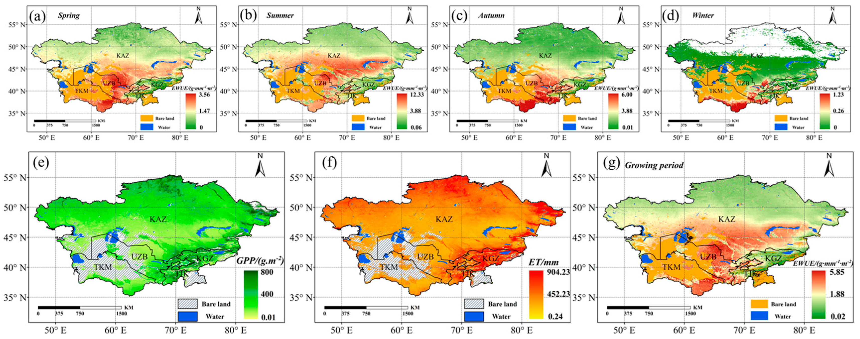
EWUE had a minor decreasing trend; both SWUE and PWUE exhibited a negligible upward trend. The seasonal change of EWUE and PWUE was summer > spring > autumn >winter. EWUE (R = −0.49) was negatively correlated with the altitude factor, whereas SWUE (R = 0.37) and PWUE (R = 0.66) had a positive connection.
(2)
The sensitivity of NDVI was consistent with the spatial patterns of precipitation. The sensitivity threshold range for different types of WUE to precipitation was about 200 mm or 1600 mm (low-value valley point) and about 300 mm or 1500 mm (high-value peak point). The optimal temperature thresholds for WUE turning-point adjustments were between 3 and 6 °C (high-value peak point) and 9 to 12 °C (low-value valley point).
(3)
The extent to which vegetation use efficiency was affected by precipitation was positively correlated with time lag, while temperature was inversely correlated. The hilly areas had a very long WUE time lag and were less affected by drought, while the plains and desert areas were the opposite. The key regulating elements impacting PWUE-SPEI were changes in water conditions. Temperature changes also formed the principal regulating factors for EWUE-SPEI and SWUE-PDSI in locations with little vegetation cover.

Supplementary Materials

The following supporting information can be downloaded at: https://www.mdpi.com/article/10.3390/rs14235999/s1, Figure S1. The inter-annual variation of WUE and climate factors in Central Asia and the seasonal variation of WUE from 2000 to 2018 ((a) Interannual variation of WUE (b) Intra-year seasonal variation of WUE); Figure S2. The spatial distribution patterns of EWUE, SWUE, and PWUE in Central Asia from 2000 to 2018 ((a) Average EWUE (b) EWUE trend (c) Average SWUE (d) SWUE trend (e) Average PWUE (f) PWUE trend); Figure S3. Spatial distribution of vegetation water use efficiency by season and growing period in Central Asia from 2000 to 2018((a,d,g,j,m) are the interannual mean of EWUE spring, summer, fall, winter and growing period; (b,e,h,k,n) are the interannual mean of SWUE spring, summer, fall, winter and growing season; (c,f,i,l,o) are the interannual mean of PWUE spring, summer, fall, winter and growing season); Figure S4. The sensitivity coefficients of EWUE, SWUE and PWUE to climatic factors (temperature, precipitation and NDVI) in Central Asia from 2000 to 2018((a–c) are the sensitivities of EWUE with respect to precipitation, temperature and NDVI, respectively; (d–f) are the sensitivities of SWUE with respect to precipitation, temperature and NDVI, respectively; (g–i) are the sensitivities of PWUE with respect to precipitation, temperature and NDVI, respectively).

Author Contributions

All authors made significant contributions to this study. Conceptualization, X.H. and J.X.; formal analysis, H.H. and P.M.K.; funding acquisition, X.H. and Z.L.; methodology, H.H. and Y.C.; project administration, J.X.; writing—original draft, H.H. and H.Z.; writing—review and editing, H.H. and Z.L. All authors have read and agreed to the published version of the manuscript.

Funding

This research was supported by the Cross Team Project of the “Light of West China” Program of CAS (No.: E0284101).

Data Availability Statement

Not applicable.

Conflicts of Interest

The authors declare that they have no known competing financial interests or personal relationships that could have appeared to influence the work reported in this paper.

Abbreviations

εPreSensitivity of WUE to Precipitation
εTemSensitivity of WUE to Temperature
εNDVISensitivity of WUE to NDVI
ASTER-GDEMAdvanced Spaceborne Thermal Emission and Reflection Radiometer Global Digital Elevation Model
CRUClimatic Research Unit
CO2(Chemical formula)Carbon Dioxide
DEMDigital Elevation Model
ECEddy Covariance
ECMWF—C3SThe European Centre for Medium-Range Weather Forecasts Copernicus Climate Change Service Center
ERA5The fifth generation of European Reanalysis of the Global Climate
ETEvapotranspiration
GEEGoogle Earth Engine
GPPGross Primary Productivity
IGBPInternational Geosphere and Biosphere Project
KAZKazakhstan
KGZKyrgyzstan
LCCMaximum Time-delay Correlation Coefficient
LPCCMaximum Time-delay Partial Correlation Coefficient
MKMann-Kendall
MODIS
NDVI
Moderate-resolution Imaging Spectroradiometer
Normalized Difference Vegetation Index
RWTCorrelation Coefficients between WUE and Monthly Mean Temperature
RWPCorrelation Coefficients between WUE and Monthly Mean Precipitation
RTPCorrelation Coefficients between Monthly Mean Temperature and Monthly Mean Precipitation
R(Cor)Pearson Correlation Coefficient
PDSIPalmer Drought Severity Index
PETPotential Evapotranspiration
PrePrecipitation
SDGsUnited Nations Sustainable Development Goals
SMSoil Moisture
SMUESoil Moisture Use Efficiency
SPEIStandardized Precipitation Evapotranspiration Index
SWSoil Water
SWUESoil Water Use Efficiency
TemTemperature
TJKTajikistan
TKMTurkmenistan
UZBUzbekistan
WUEWater Use Efficiency
EWUEEcosystem Water Use Efficiency
PWUEPrecipitation Water Use Efficiency

References

  1. Liu, R.; Dong, X.; Wang, X.; Zhang, P.; Liu, M.; Zhang, Y. Study on the relationship among the urbanization process, ecosystem services and human well-being in an arid region in the context of carbon flow: Taking the Manas river basin as an example. Ecol. Indic. 2021, 132, 108248. [Google Scholar] [CrossRef]
  2. Zou, J.; Ding, J.; Welp, M.; Huang, S.; Liu, B. Assessing the Response of Ecosystem Water Use Efficiency to Drought During and after Drought Events across Central Asia. Sensors 2020, 20, 581. [Google Scholar] [CrossRef] [Green Version]
  3. Viets, F.G., Jr. Increasing water use efficiency by soil management. In Plant Environment and Efficient Water Use; John Wiley & Sons, Inc.: Hoboken, NJ, USA, 1966; pp. 259–274. [Google Scholar]
  4. Adams, M.A.; Turnbull, T.L.; Sprent, J.I.; Buchmann, N. Legumes are different: Leaf nitrogen, photosynthesis, and water use efficiency. Proc. Natl. Acad. Sci. USA 2016, 113, 4098–4103. [Google Scholar] [CrossRef] [PubMed] [Green Version]
  5. Knauer, J.U.R.; Zaehle, S.O.N.; Reichstein, M.; Medlyn, B.E.; Forkel, M.; Hagemann, S.; Werner, C. The response of ecosystem water-use efficiency to rising atmospheric CO 2 concentrations: Sensitivity and large-scale biogeochemical implications. New Phytol. 2017, 213, 1654–1666. [Google Scholar] [CrossRef] [PubMed] [Green Version]
  6. Li, Y.; Fan, J.; Hu, Z.; Shao, Q.; Harris, W. Comparison of evapotranspiration components and water-use efficiency among different land use patterns of temperate steppe in the Northern China pastoral-farming ecotone. Int. J. Biometeorol. 2016, 60, 827–841. [Google Scholar] [CrossRef]
  7. Tian, H.; Chen, G.; Liu, M.; Zhang, C.; Sun, G.; Lu, C.; Xu, X.; Ren, W.; Pan, S.; Chappelka, A. Model estimates of net primary productivity, evapotranspiration, and water use efficiency in the terrestrial ecosystems of the southern United States during 1895–2007. For. Ecol. Manag. 2010, 259, 1327. [Google Scholar] [CrossRef]
  8. Farquhar, G.D.; Sharkey, T.D. Stomatal Conductance and Photosynthesis. Annu. Rev. Plant Physiol. 1982, 33, 317–345. [Google Scholar] [CrossRef]
  9. Xue, B.; Guo, Q.; Otto, A.; Xiao, J.; Tao, S.; Li, L. Global patterns, trends, and drivers of water use efficiency from 2000 to 2013. Ecosphere 2015, 6, 1–18. [Google Scholar] [CrossRef]
  10. Yang, Y.; Guan, H.; Batelaan, O.; McVicar, T.R.; Long, D.; Piao, S.; Liang, W.; Liu, B.; Jin, Z.; Simmons, C.T. Contrasting responses of water use efficiency to drought across global terrestrial ecosystems. Sci. Rep. 2016, 6, 23284. [Google Scholar] [CrossRef] [Green Version]
  11. Brümmer, C.; Black, T.A.; Jassal, R.S.; Grant, N.J.; Spittlehouse, D.L.; Chen, B.; Nesic, Z.; Amiro, B.D.; Arain, M.A.; Barr, A.G.; et al. How climate and vegetation type influence evapotranspiration and water use efficiency in Canadian forest, peatland and grassland ecosystems. Agric. For. Meteorol. 2012, 153, 14–30. [Google Scholar] [CrossRef]
  12. He, B.; Wang, H.; Huang, L.; Liu, J.; Chen, Z. A new indicator of ecosystem water use efficiency based on surface soil moisture retrieved from remote sensing. Ecol. Indic. 2017, 75, 10–16. [Google Scholar] [CrossRef] [Green Version]
  13. Huang, M.; Piao, S.; Zeng, Z.; Peng, S.; Ciais, P.; Cheng, L.; Mao, J.; Poulter, B.; Shi, X.; Yao, Y.; et al. Seasonal responses of terrestrial ecosystem water-use efficiency to climate change. Glob. Chang. Biol. 2016, 22, 2165–2177. [Google Scholar] [CrossRef]
  14. Huang, M.; Piao, S.; Sun, Y.; Ciais, P.; Cheng, L.; Mao, J.; Poulter, B.; Shi, X.; Zeng, Z.; Wang, Y. Change in terrestrial ecosystem water-use efficiency over the last three decades. Glob. Chang. Biol. 2015, 21, 2366–2378. [Google Scholar] [CrossRef]
  15. Zhang, T.; Peng, J.; Liang, W.; Yang, Y.; Liu, Y. Spatial–temporal patterns of water use efficiency and climate controls in China’s Loess Plateau during 2000–2010. Sci. Total Environ. 2016, 565, 105–122. [Google Scholar] [CrossRef] [PubMed]
  16. Kato, T.; Tang, Y. Spatial variability and major controlling factors of CO2 sink strength in Asian terrestrial ecosystems: Evidence from eddy covariance data. Glob. Chang. Biol. 2008, 14, 2333–2348. [Google Scholar] [CrossRef]
  17. White, M.A.; Brunsell, N.; Schwartz, M.D. Vegetation Phenology in Global Change Studies. In Phenology an Integrative Environmental Science; Springer: Berlin/Heidelberg, Germany, 2003; Volume 39, pp. 453–466. [Google Scholar]
  18. Zonn, L.S.; Andrey, G.K. The Turkmen Lake Altyn Asyr and Water Resources in Turkmenistan. In The Handbook of Environmental Chemistry; Springer: Berlin/Heidelberg, Germany, 2013. [Google Scholar]
  19. Li, X.; Farooqi, T.J.A.; Jiang, C.; Liu, S.; Sun, O.J. Spatiotemporal variations in productivity and water use efficiency across a temperate forest landscape of Northeast China. For. Ecosyst. 2019, 6, 22. [Google Scholar] [CrossRef] [Green Version]
  20. Wonkka, C.L.; Twidwell, D.; Franz, T.E.; Taylor, C.A., Jr.; Rogers, W.E. Persistence of a severe drought increases desertification but not woody dieback in semiarid savanna. Rangel Ecol. Manag. 2016, 69, 491–498. [Google Scholar] [CrossRef]
  21. Rietkerk, M.; Dekker, S.C.; De Ruiter, P.C.; van de Koppel, J. Self-organized patchiness and catastrophic shifts in ecosystems. Science 2004, 305, 1926–1929. [Google Scholar] [CrossRef] [Green Version]
  22. Zou, J.; Ding, J.; Welp, M.; Huang, S.; Liu, B. Using MODIS data to analyse the ecosystem water use efficiency spatial-temporal variations across Central Asia from 2000 to 2014. Environ. Res. 2020, 182, 108985. [Google Scholar] [CrossRef]
  23. Zhu, S.; Zhang, C.; Fang, X.; Cao, L. Interactive and individual effects of multi-factor controls on water use efficiency in Central Asian ecosystems. Environ. Res. Lett. 2020, 15, 84025. [Google Scholar] [CrossRef]
  24. Han, Q.; Li, C.; Zhao, C.; Zhang, Y.; Li, S. Grazing decreased water use efficiency in Central Asia from 1979 to 2011. Ecol. Model. 2018, 388, 72–79. [Google Scholar] [CrossRef]
  25. Hu, Z.; Zhang, C.; Hu, Q.; Tian, H. Temperature changes in Central Asia from 1979 to 2011 based on multiple datasets. J. Clim. 2014, 27, 1143–1167. [Google Scholar] [CrossRef]
  26. Justice, C.O.; Townshend, J.; Vermote, E.F.; Masuoka, E.; Wolfe, R.E.; Saleous, N.; Roy, D.P.; Morisette, J.T. An overview of MODIS Land data processing and product status. Remote Sens. Environ. 2002, 83, 3–15. [Google Scholar] [CrossRef]
  27. Hersbach, H.; Bell, B.; Berrisford, P.; Hirahara, S.; Hor, A.; Nyi, A.A.S.; Mu, N.; Oz-Sabater, J.I.N.; Nicolas, J.; Peubey, C.; et al. The ERA5 global reanalysis. Q. J. Roy. Meteor. Soc. 2020, 146, 1999–2049. [Google Scholar] [CrossRef]
  28. Harris, I.; Jones, P.D.; Osborn, T.J.; Lister, D.H. Updated high-resolution grids of monthly climatic observations—The CRU TS3. 10 Dataset. Int. J. Climatol. 2014, 34, 623–642. [Google Scholar] [CrossRef] [Green Version]
  29. Zheng, H.; Zhang, L.; Zhu, R.; Liu, C.; Sato, Y.; Fukushima, Y. Responses of streamflow to climate and land surface change in the headwaters of the Yellow River Basin. Water Resour. Res. 2009, 45, 641–648. [Google Scholar] [CrossRef]
  30. Juki, C.D.; Deni, C.; Juki, C.V. Investigating relationships between rainfall and karst-spring discharge by higher-order partial correlation functions. J. Hydrol. 2015, 530, 24–36. [Google Scholar] [CrossRef]
  31. Wu, D.; Zhao, X.; Liang, S.; Zhou, T.; Huang, K.; Tang, B.; Zhao, W. Time-lag effects of global vegetation responses to climate change. Glob. Chang. Biol. 2015, 21, 3520–3531. [Google Scholar] [CrossRef]
  32. Benesty, J.; Chen, J.; Huang, Y.; Cohen, I. Pearson correlation coefficient. In Noise Reduction in Speech Processing; Springer: Berlin/Heidelberg, Germany, 2009; pp. 1–4. [Google Scholar]
  33. Vicente-Serrano, S.M.; Beguería, S.; López-Moreno, J.I. A Multiscalar Drought Index Sensitive to Global Warming: The Standardized Precipitation Evapotranspiration Index. J. Clim. 2010, 23, 1696–1718. [Google Scholar] [CrossRef] [Green Version]
  34. Trenberth, K.E.; Dai, A.; Gerard, V.D.S.; Jones, P.D.; Barichivich, J.; Briffa, K.R.; Sheffield, J. Global warming and changes in drought. Nat. Clim. Chang. 2013, 4, 17–22. [Google Scholar] [CrossRef]
  35. Ayantobo, O.O.; Li, Y.; Song, S.; Yao, N. Spatial comparability of drought characteristics and related return periods in mainland China over 1961–2013. J. Hydrol. 2017, 550, 549–567. [Google Scholar] [CrossRef]
  36. Bastos, A.; Fu, Z.; Ciais, P.; Friedlingstein, P.; Sitch, S.; Pongratz, J.; Weber, U.; Reichstein, M.; Anthoni, P.; Arneth, A.; et al. Impacts of extreme summers on European ecosystems: A comparative analysis of 2003, 2010 and 2018. Philos. Trans. R. Soc. B 2020, 375, 20190507. [Google Scholar] [CrossRef]
  37. Schaefer, K.; Schwalm, C.R.; Williams, C.; Arain, M.A.; Barr, A.; Chen, J.M.; Davis, K.J.; Dimitrov, D.; Hilton, T.W.; Hollinger, D.Y.; et al. A model-data comparison of gross primary productivity: Results from the North American Carbon Program site synthesis. J. Geophys. Res. Biogeosci. 2012, 117, G03010. [Google Scholar] [CrossRef] [Green Version]
  38. Aires, L.M.I.; Pio, C.A.; Pereira, J.S. Carbon dioxide exchange above a Mediterranean C3/C4 grassland during two climatologically contrasting years. Glob. Chang. Biol. 2008, 14, 539–555. [Google Scholar] [CrossRef] [Green Version]
  39. Zheng, H.; Lin, H.; Zhu, X.; Jin, Z.; Bao, H. Divergent spatial responses of plant and ecosystem water-use efficiency to climate and vegetation gradients in the Chinese Loess Plateau. Glob. Planet. Chang. 2019, 181, 102995. [Google Scholar] [CrossRef]
  40. Zhu, X.; Yu, G.; Wang, Q.; Hu, Z.; Zheng, H.; Li, S.; Sun, X.; Zhang, Y.; Yan, J.; Wang, H.; et al. Spatial variability of water use efficiency in China’s terrestrial ecosystems. Glob. Planet. Chang. 2015, 129, 37–44. [Google Scholar] [CrossRef]
  41. Ma, Q.; Zhang, J.; Game, A.T.; Chang, Y.; Li, S. Spatiotemporal variability of summer precipitation and precipitation extremes and associated large-scale mechanisms in Central Asia during 1979–2018. J. Hydrol. X 2020, 8, 100061. [Google Scholar] [CrossRef]
  42. Jennings, K.S.; Winchell, T.S.; Livneh, B.; Molotch, N.P. Spatial variation of the rain-snow temperature threshold across the Northern Hemisphere. Nat. Commun. 2018, 9, 1148. [Google Scholar] [CrossRef] [Green Version]
  43. Hao, X.; Ma, H.; Hua, D.; Qin, J.; Zhang, Y. Response of ecosystem water use efficiency to climate change in the Tianshan Mountains, Central Asia. Environ. Monit. Assess. 2019, 191, 561. [Google Scholar] [CrossRef] [PubMed]
  44. Schwartz, R.C.; Baumhardt, R.L.; Evett, S.R. Tillage effects on soil water redistribution and bare soil evaporation throughout a season. Soil Tillage Res. 2010, 110, 221–229. [Google Scholar] [CrossRef]
  45. Liu, W.; Mo, X.; Liu, S.; Lin, Z.; Lv, C. Attributing the changes of grass growth, water consumed and water use efficiency over the Tibetan Plateau. J. Hydrol. 2021, 598, 126464. [Google Scholar] [CrossRef]
  46. Liu, N.; Sun, P.; Caldwell, P.V.; Harper, R.; Liu, S.; Sun, G. Trade-off between watershed water yield and ecosystem productivity along elevation gradients on a complex terrain in southwestern China. J. Hydrol. 2020, 590, 125449. [Google Scholar] [CrossRef]
  47. Krich, C.; Mahecha, M.D.; Migliavacca, M.; De Kauwe, M.G.; Griebel, A.; Runge, J.; Miralles, D.G. Decoupling between ecosystem photosynthesis and transpiration: A last resort against overheating. Environ. Res. Lett. 2022, 17, 44013. [Google Scholar] [CrossRef]
  48. Tang, X.; Li, H.; Desai, A.R.; Nagy, Z.; Luo, J.; Kolb, T.E.; Olioso, A.; Xu, X.; Yao, L.; Kutsch, W.; et al. How is water-use efficiency of terrestrial ecosystems distributed and changing on Earth? Sci. Rep. 2014, 4, 7483. [Google Scholar] [CrossRef] [PubMed] [Green Version]
  49. Hao, H.; Li, Z.; Chen, Y.; Xu, J.; Li, S.; Zhang, S. Recent variations in soil moisture use efficiency (SMUE) and its influence factors in Asian drylands. J. Clean. Prod. 2022, 373, 133860. [Google Scholar] [CrossRef]
  50. Zhan, L.; Shen, T.; Chen, H.; Gu, L.; Zhou, H.; Feng, Q.; Yang, L.; Zhao, N.; Feng, Y. Evaporation Characteristics of a Single Desulfurization Wastewater Droplet in High-temperature Gas. Int. J. Heat Mass Tran. 2022, 185, 122317. [Google Scholar] [CrossRef]
  51. Kim, H.; Wigneron, J.; Kumar, S.; Dong, J.; Wagner, W.; Cosh, M.H.; Bosch, D.D.; Collins, C.H.; Starks, P.J.; Seyfried, M.; et al. Global scale error assessments of soil moisture estimates from microwave-based active and passive satellites and land surface models over forest and mixed irrigated/dryland agriculture regions. Remote Sens. Environ. 2020, 251, 112052. [Google Scholar] [CrossRef]
  52. Albergel, C.; Dutra, E.; Munier, S.; Calvet, J.; Munoz-Sabater, J.; de Rosnay, P.; Balsamo, G. ERA-5 and ERA-Interim driven ISBA land surface model simulations: Which one performs better? Hydrol. Earth Syst. Sci. 2018, 22, 3515–3532. [Google Scholar] [CrossRef] [Green Version]
  53. Henttonen, H.M.; Kinen, M.A.H.; Heiskanen, J.; Peltoniemi, M.; Laur, E.N.A.; Hordo, M. Response of radial increment variation of Scots pine to temperature, precipitation and soil water content along a latitudinal gradient across Finland and Estonia. Agric. For. Meteorol. 2014, 198, 294–308. [Google Scholar] [CrossRef]
  54. Xie, J.; Chen, J.; Sun, G.; Zha, T.; Yang, B.; Chu, H.; Liu, J.; Wan, S.; Zhou, C.; Ma, H.; et al. Ten-year variability in ecosystem water use efficiency in an oak-dominated temperate forest under a warming climate. Agric. For. Meteorol. 2016, 218, 209–217. [Google Scholar] [CrossRef]
  55. Pei, T.; Li, X.; Wu, H.; Wu, X.; Chen, Y.; Xie, B. Sensitivity of vegetation water use efficiency to climate and vegetation index in Loess Plateau, China. Trans. Chin. Soc. Agric. Eng. 2019, 35, 119–125. (In Chinese) [Google Scholar]
  56. Zhou, Y.; Zhang, J.; Yin, C.; Huang, H.; Sun, S.; Meng, P. Empirical analysis of the influences of meteorological factors on the interannual variations in carbon fluxes of a Quercus variabilis plantation. Agric. For. Meteorol. 2022, 326, 109190. [Google Scholar] [CrossRef]
  57. Reichstein, M.; Camps-Valls, G.; Stevens, B.; Jung, M.; Denzler, J.; Carvalhais, N. Deep learning and process understanding for data-driven Earth system science. Nature 2019, 566, 195–204. [Google Scholar] [CrossRef] [PubMed]
  58. Sun, Y.; Piao, S.; Huang, M.; Ciais, P.; Zeng, Z.; Cheng, L.; Li, X.; Zhang, X.; Mao, J.; Peng, S.; et al. Global patterns and climate drivers of water-use efficiency in terrestrial ecosystems deduced from satellite-based datasets and carbon cycle models. Glob. Ecol. Biogeogr. 2016, 25, 311–323. [Google Scholar] [CrossRef] [Green Version]
  59. Li, J.; Deng, J.; Zhou, Y.; Yin, Y.; Wei, Y.; Jing, Y.; Zhang, R. Water-use Efficiency of Typical Afforestation Tree Species in Liaoning, PR China and Their Response to Environmental Factors. Nat. Environ. Pollut. Technol. 2016, 15, 1427. [Google Scholar]
  60. Pradawet, C.; Khongdee, N.; Pansak, W.; Spreer, W.; Hilger, T.; Cadisch, G. Thermal imaging for assessment of maize water stress and yield prediction under drought conditions. J. Agron. Crop Sci. 2022. [Google Scholar] [CrossRef]
  61. Kersebaum, K.C.; Stöckle, C.O. Simulation of Climate Change Effects on Evapotranspiration, Photosynthesis, Crop Growth, and Yield Processes in Crop Models. In Modeling Processes and Their Interactions in Cropping Systems: Challenges for the 21st Century; John Wiley & Sons, Inc.: Hoboken, NJ, USA, 2022; pp. 291–331. [Google Scholar]
Figure 1. Location of the study area: (a) Temperature and precipitation in longitude, (b) temperature, (c) landcover, (d) temperature and precipitation in latitude, (e) precipitation, and (f) DEM. Drawing NO.: GS (2016) 2966.
Remotesensing 14 05999 g001
Figure 2. Spatial distribution patterns of EWUE in Central Asia from 2000 to 2018: (ad) average EWUE in spring, summer, autumn and winter, (e) annual average GPP, (f) annual average ET, (g) average EWUE in the growing period.
Remotesensing 14 05999 g002
Figure 3. (a) Vertical gradients of EWUE, SWUE and PWUE, (b) comparison of EWUE, SWUE and PWUE values for different vegetation types, and (c) comparison of temperature and precipitation values for different vegetation types in Central Asia from 2000 to 2018.
Remotesensing 14 05999 g003
Figure 4. Sensitivity coefficients of WUEs to climatic factors: (a) precipitation and NDVI in Central Asia from 2000 to 2018; (b) temperature and NDVI in Central Asia from 2000 to 2018.
Remotesensing 14 05999 g004
Figure 5. Maximum time-delay partial correlation coefficient: (a) PWUE, (c) SWUE, (e) EWUE and lag time, (b) PWUE, (d) SWUE, (f) EWUE between WUE and precipitation in Central Asia from 2000 to 2018. Partial correlation coefficient: (g) PWUE, (i) SWUE, (k) EWUE and lag time, (h) PWUE, (j) SWUE, (l) EWUE between WUE of different vegetation types and maximum time delay of precipitation. (LPCC: Maximum time-delay partial correlation coefficient.).
Remotesensing 14 05999 g005
Figure 6. Maximum time-delay partial correlation coefficient: (a) PWUE, (c) SWUE, (e) EWUE and lag time, (b) PWUE, (d) SWUE, (f) EWUE between WUE and temperature in Central Asia from 2000 to 2018. Partial correlation coefficient: (g) PWUE, (i) SWUE, (k) EWUE and lag time, (h) PWUE, (j) SWUE, (l) EWUE between WUE of different vegetation types and maximum time delay of temperature.
Remotesensing 14 05999 g006
Figure 7. Maximum time-delay correlation coefficient: (a) EW-SPEI, (c) PW-SPEI, (e) SW-PDSI and lag time, (b) EW-SPEI, (d) PW-SPEI, (f) SW-PDSI between WUE and drought (SPEI and PDSI) in Central Asia. (LCC: Maximum time-delay correlation coefficient.).
Remotesensing 14 05999 g007
Table 1. Data Product Type and Source.
SerieProductTypeTemporal ResolutionSpatial ResolutionSource URL
MODISMOD17A2GPP8 d500 mhttps://modis.gsfc.nasa.gov/ (accessed on 5 January 2020)
MOD16A2ET8 d500 mhttps://modis.gsfc.nasa.gov/ (accessed on 5 January 2020)
MOD13A3NDVI30 d500 mhttps://modis.gsfc.nasa.gov/ (accessed on 5 January 2020)
MCD12Q1Landcover (IGBP)96 d500 mhttps://modis.gsfc.nasa.gov/ (accessed on 5 January 2020)
ASTER -GDEMDEM201130 mhttp://www.gdem.aster.ersdac.or.jp/index.jsp (accessed on 15 February 2020)
ERA5ERA5Soil watermonthly0.1°https://www.ecmwf.int (accessed on 17 March 2021)
ERA5Premonthly0.1°https://www.ecmwf.int (accessed on 17 March 2021)
ERA5Temperaturemonthly0.1°https://www.ecmwf.int (accessed on 17 March 2021)
CRUCRU4.2.1Premonthly0.5°https://www.uea.ac.uk/ (accessed on 20 March 2021)
CRU4.2.1PETmonthly0.5°https://www.uea.ac.uk/ (accessed on 20 March 2021)
CRU4.2.1PDSImonthly0.5°https://www.uea.ac.uk/ (accessed on 20 March 2021)
Note: The paper adopts the land use classification system of the IGBP (International Geosphere and Biosphere Project). According to vegetation types in Central Asia, the WUE grid situation is classified as forestland (accounting for 0.34% of the entire vegetation area), shrub (2.81%), grassland (85.73%), wetland (0.12%), and crops (6.26%).
Table 2. EWUE Seasonal Sensitivity and Contribution Rate to Temperature, Precipitation and NDVI.
SpringSummerAutumnWinter
S-CoefCon-RateS-CoefCon-RateS-CoefCon-RateS-CoefCon-Rate
Pre11.4059.65%−0.377.02%−3.04−91.27%−0.020.14%
Tem0.8066.16%0.200.28%0.93−93.03%−1.040.08%
NDVI1.6866.02%−1.207.93%4.70−92.81%−0.010.54%
Table 3. Time-delay Correlation Coefficient and Time Lag of WUE Response to Drought in Central Asia.
Time-Lag CorrelationLag Time/MonthVeg-TypesTime-Lag CorrelationLag Time/MonthElevationTime-Lag CorrelationLag Time/Month
EW-SPEIPW-SPEISW-PDSIEWPWSW EW-SPEIPW-SPEISW-PDSIEWPWSW EW-SPEIPW-SPEISW-PDSIEWPWSW
KAZ−0.3170.4250.2511.832.361.4Forest0.4940.70.6321.241.291.69AL10.6060.8230.642.881.661.7
TJK0.1230.4360.3072.72.592.17Shrub0.6280.4560.3550.332.711.51AL20.380.5450.4562.192.21.39
KGZ0.5030.6770.2651.072.281.83Grass0.3580.550.462.312.161.44AL30.3490.5310.4652.092.211.43
UZB0.5350.4640.3380.532.531.82Wetlands0.3150.3570.481.892.371.3AL40.1480.5010.3472.462.282.02
TKM0.3650.5530.4952.452.131.38Crops0.2880.50.4332.222.541.69
Note: AL1: −288~0 m; AL2: 0~500 m; AL3: 500~1000 m; AL4: 1000~7021 m.
Publisher’s Note: MDPI stays neutral with regard to jurisdictional claims in published maps and institutional affiliations.

