
Evaluating Data Inter-Operability of Multiple UAV–LiDAR Systems for Measuring the 3D Structure of Savanna Woodland

 ,
,  ,
,  , , , , and
Abstract
1. Introduction
2. Materials and Methods
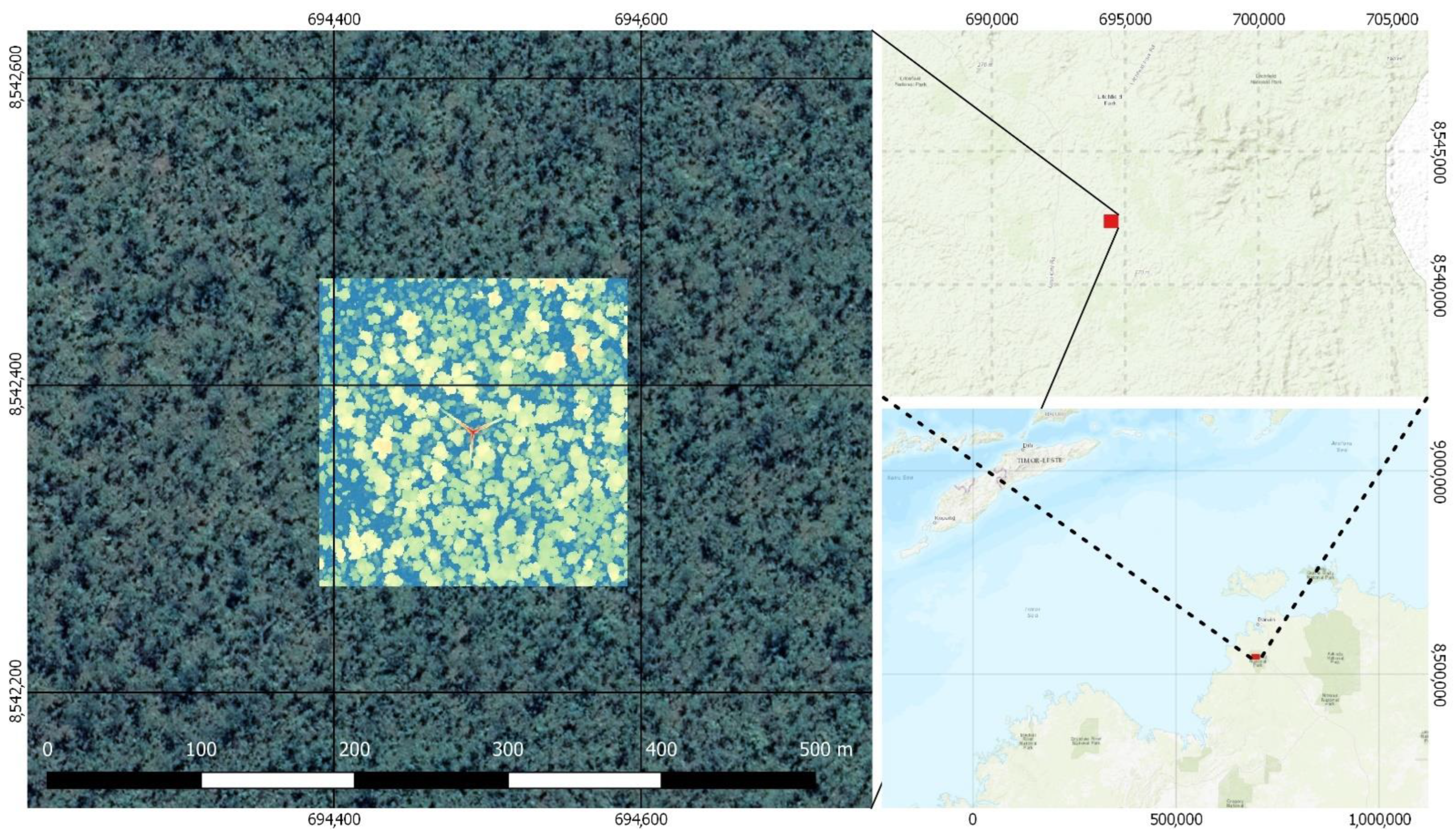
2.1. Study Area
2.2. UAV–LiDAR Sensors
2.3. Data Acquisition and Pre-Processing
2.4. Analysis

| Variable/Metric | Method | Function | Package/Software |
|---|---|---|---|
| DTM | KNNIDW on ground points (k = 6, p = 2) | rasterize_terrain | R: lidR |
| CHM | Local maximum calculation | grid_canopy | R: lidR |
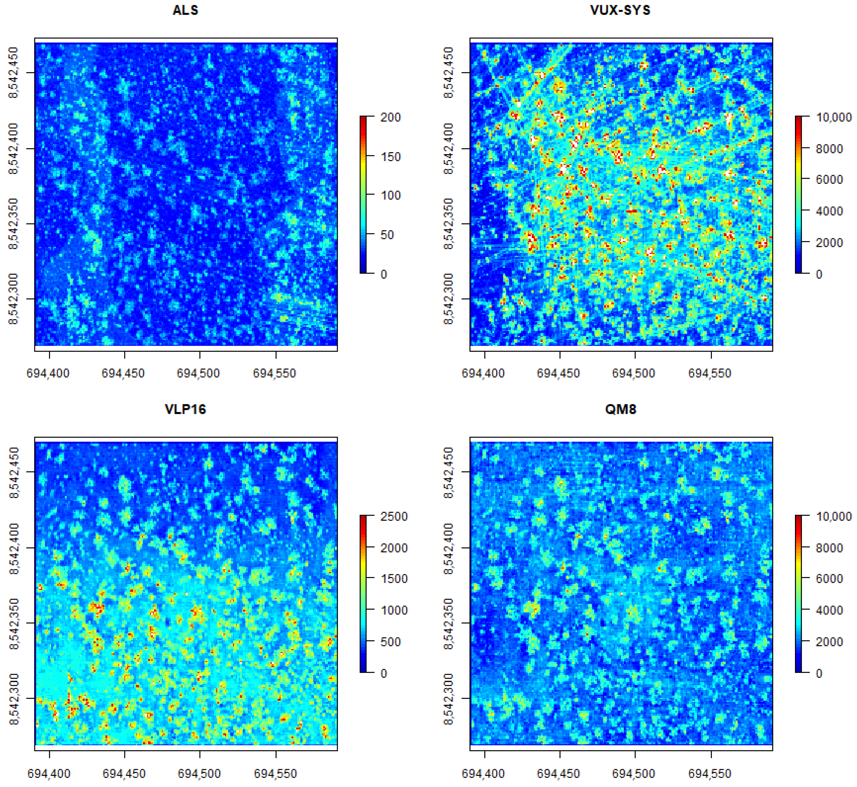
| Point density | Point counts per grid cell | grid_density | R: lidR |
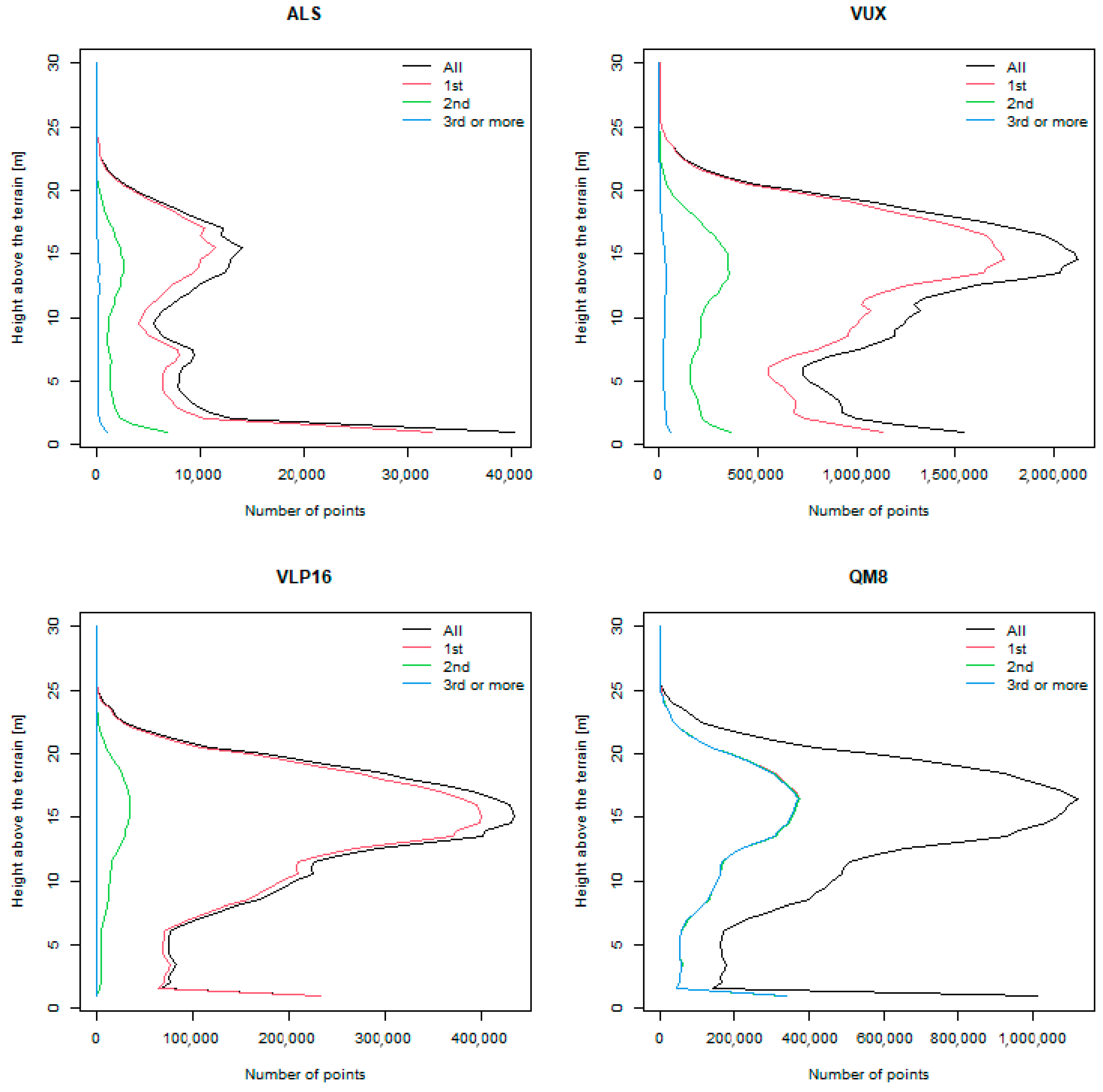
| Frequency profiles | Point counts in 0.5 m Z-bins above the terrain | R | |
| Canopy cover | Number of first returns above the height cutoff divided by the number of all first returns, output as a percentage. | Lascanopy | Lastools |
| Gap fraction profiles | In which: N[0;z] being the number of returns below z, Ntotal is the total number of returns, N[0;z+dz] is the number of returns below z + dz | gap_fraction_profile | R: lidR [28] |
| Tree height | Tree height = Zmax − Zmin | tree_height_pc | R: ITSME [29] |
| Tree projection Area | Concave Hull fitting (concavity = 2) | R: ITSMe [29] | |
| Tree volume | 3D alpha shape fitting (alpha = 2) | alpha_volume_pc | R: ITSMe [29] |
3. Results
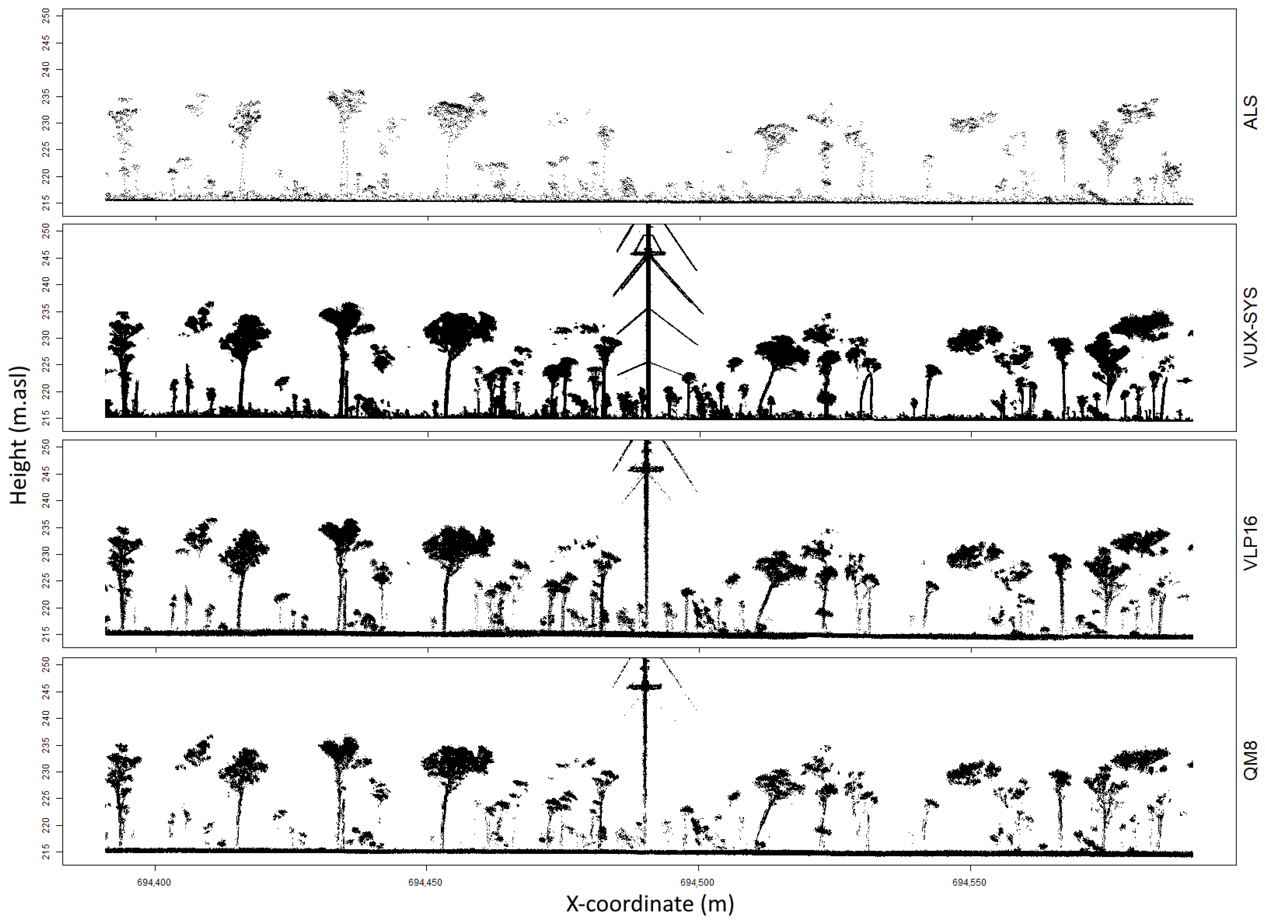
3.1. Point Clouds
3.2. Digital Terrain Models
3.3. Canopy Metrics
3.4. Individual Tree Parameter Estimation
4. Discussion
5. Conclusions
Author Contributions
Funding
Data Availability Statement
Acknowledgments
Conflicts of Interest
References
- Goodwin, N.R.; Coops, N.C.; Culvenor, D.S. Assessment of forest structure with airborne LiDAR and the effects of platform altitude. Remote Sens. Environ. 2006, 103, 140–152. [Google Scholar] [CrossRef]
- Zhang, Z.; Cao, L.; She, G. Estimating forest structural parameters using canopy metrics derived from airborne LiDAR data in subtropical forests. Remote Sens. 2017, 9, 940. [Google Scholar] [CrossRef]
- Simard, M.; Pinto, N.; Fisher, J.B.; Baccini, A. Mapping forest canopy height globally with spaceborne lidar. J. Geophys. Res. Biogeosci. 2011, 116, 103592. [Google Scholar] [CrossRef]
- Tang, H.; Armston, J.; Hancock, S.; Marselis, S.; Goetz, S.; Dubayah, R. Characterizing global forest canopy cover distribution using spaceborne lidar. Remote Sens. Environ. 2019, 231, 111262. [Google Scholar] [CrossRef]
- Calders, K.; Adams, J.; Armston, J.; Bartholomeus, H.; Bauwens, S.; Bentley, L.P.; Chave, J.; Danson, F.M.; Demol, M.; Disney, M. Terrestrial laser scanning in forest ecology: Expanding the horizon. Remote Sens. Environ. 2020, 251, 112102. [Google Scholar] [CrossRef]
- Bauwens, S.; Bartholomeus, H.; Calders, K.; Lejeune, P. Forest inventory with terrestrial LiDAR: A comparison of static and hand-held mobile laser scanning. Forests 2016, 7, 127. [Google Scholar] [CrossRef]
- Terryn, L.; Calders, K.; Bartholomeus, H.; Bartolo, R.E.; Brede, B.; D’hont, B.; Disney, M.; Herold, M.; Lau, A.; Shenkin, A. Quantifying tropical forest structure through terrestrial and UAV laser scanning fusion in Australian rainforests. Remote Sens. Environ. 2022, 271, 112912. [Google Scholar] [CrossRef]
- Côté, J.-F.; Fournier, R.A.; Egli, R. An architectural model of trees to estimate forest structural attributes using terrestrial LiDAR. Environ. Model. Softw. 2011, 26, 761–777. [Google Scholar] [CrossRef]
- Neuville, R.; Bates, J.S.; Jonard, F. Estimating forest structure from UAV-mounted LiDAR point cloud using machine learning. Remote Sens. 2021, 13, 352. [Google Scholar] [CrossRef]
- Liu, K.; Shen, X.; Cao, L.; Wang, G.; Cao, F. Estimating forest structural attributes using UAV-LiDAR data in Ginkgo plantations. ISPRS J. Photogramm. Remote Sens. 2018, 146, 465–482. [Google Scholar] [CrossRef]
- Wallace, L.; Lucieer, A.; Malenovský, Z.; Turner, D.; Vopěnka, P. Assessment of forest structure using two UAV techniques: A comparison of airborne laser scanning and structure from motion (SfM) point clouds. Forests 2016, 7, 62. [Google Scholar] [CrossRef]
- Brede, B.; Lau, A.; Bartholomeus, H.M.; Kooistra, L. Comparing RIEGL RiCOPTER UAV LiDAR derived canopy height and DBH with terrestrial LiDAR. Sensors 2017, 17, 2371. [Google Scholar] [CrossRef] [PubMed]
- Hu, T.; Sun, X.; Su, Y.; Guan, H.; Sun, Q.; Kelly, M.; Guo, Q. Development and performance evaluation of a very low-cost UAV-LiDAR system for forestry applications. Remote Sens. 2020, 13, 77. [Google Scholar] [CrossRef]
- Wallace, L.; Lucieer, A.; Watson, C.; Turner, D. Development of a UAV-LiDAR system with application to forest inventory. Remote Sens. 2012, 4, 1519–1543. [Google Scholar] [CrossRef]
- Gyawali, A.; Aalto, M.; Peuhkurinen, J.; Villikka, M.; Ranta, T. Comparison of Individual Tree Height Estimated from LiDAR and Digital Aerial Photogrammetry in Young Forests. Sustainability 2022, 14, 3720. [Google Scholar] [CrossRef]
- Ganz, S.; Käber, Y.; Adler, P. Measuring tree height with remote sensing—A comparison of photogrammetric and LiDAR data with different field measurements. Forests 2019, 10, 694. [Google Scholar] [CrossRef]
- Thiel, C.; Schmullius, C. Comparison of UAV photograph-based and airborne lidar-based point clouds over forest from a forestry application perspective. Int. J. Remote Sens. 2017, 38, 2411–2426. [Google Scholar] [CrossRef]
- Moe, K.T.; Owari, T.; Furuya, N.; Hiroshima, T. Comparing individual tree height information derived from field surveys, LiDAR and UAV-DAP for high-value timber species in Northern Japan. Forests 2020, 11, 223. [Google Scholar] [CrossRef]
- Levick, S.R.; Whiteside, T.; Loewensteiner, D.A.; Rudge, M.; Bartolo, R. Leveraging TLS as a Calibration and Validation Tool for MLS and ULS Mapping of Savanna Structure and Biomass at Landscape-Scales. Remote Sens. 2021, 13, 257. [Google Scholar] [CrossRef]
- Hyyppä, E.; Yu, X.; Kaartinen, H.; Hakala, T.; Kukko, A.; Vastaranta, M.; Hyyppä, J. Comparison of backpack, handheld, under-canopy UAV, and above-canopy UAV laser scanning for field reference data collection in boreal forests. Remote Sens. 2020, 12, 3327. [Google Scholar] [CrossRef]
- Rudge, M.L.; Levick, S.R.; Bartolo, R.E.; Erskine, P.D. Modelling the diameter distribution of savanna trees with drone-based LiDAR. Remote Sens. 2021, 13, 1266. [Google Scholar] [CrossRef]
- TERN. Litchfield Savanna SuperSite. Available online: http://www.tern-supersites.net.au/supersites/lfld (accessed on 13 June 2022).
- CloudCompare; v2.11.3. [GPL Software], 2020. Available online: http://www.cloudcompare.org (accessed on 13 June 2022).
- Wilkes, P.; Lau, A.; Disney, M.; Calders, K.; Burt, A.; Gonzalez de Tanago, J.; Bartholomeus, H.; Brede, B.; Herold, M. Data acquisition considerations for Terrestrial Laser Scanning of forest plots. Remote Sens. Environ. 2017, 196, 140–153. [Google Scholar] [CrossRef]
- Roussel, J.-R.; Auty, D.; Coops, N.C.; Tompalski, P.; Goodbody, T.R.H.; Meador, A.S.; Bourdon, J.-F.; de Boissieu, F.; Achim, A. lidR: An R package for analysis of Airborne Laser Scanning (ALS) data. Remote Sens. Environ. 2020, 251, 112061. [Google Scholar] [CrossRef]
- Isenburg, M. LAStools—Efficient Tools for LiDAR Processing. 2020. Available online: https://rapidlasso.com/lastools/ (accessed on 13 June 2022).
- R Core Team. R: A Language and Environment for Statistical Computing; R Foundation for Statistical Computing: Vienna, Austria, 2010. [Google Scholar]
- Bouvier, M.; Durrieu, S.; Fournier, R.A.; Renaud, J.-P. Generalizing predictive models of forest inventory attributes using an area-based approach with airborne LiDAR data. Remote Sens. Environ. 2015, 156, 322–334. [Google Scholar] [CrossRef]
- Terryn, L.; Calders, K.; Akerblom, M.; Bartholomeus, H.; Disney, M.; Levick, S.R.; Origo, N.; Raumonen, P.; Verbeeck, H. Analysing individual 3D tree structure using the R package ITSMe. Methods Ecol. Evol. 2022, 00, 1–11. [Google Scholar] [CrossRef]
- Jalobeanu, A.; Kim, A.M.; Runyon, S.C.; Olsen, R.; Kruse, F.A. Uncertainty assessment and probabilistic change detection using terrestrial and airborne LiDAR. In Proceedings of the Laser Radar Technology and Applications XIX; and Atmospheric Propagation XI, Baltimore, MD, USA, 6–7 May 2014; pp. 228–246. [Google Scholar]
- Brede, B.; Calders, K.; Lau, A.; Raumonen, P.; Bartholomeus, H.M.; Herold, M.; Kooistra, L. Non-destructive tree volume estimation through quantitative structure modelling: Comparing UAV laser scanning with terrestrial LIDAR. Remote Sens. Environ. 2019, 233, 111355. [Google Scholar] [CrossRef]
- Duncanson, L.; Dubayah, R. Monitoring individual tree-based change with airborne lidar. Ecol. Evol. 2018, 8, 5079–5089. [Google Scholar] [CrossRef]
- Levick, S.R.; Asner, G.P. The rate and spatial pattern of treefall in a savanna landscape. Biol. Conserv. 2013, 157, 121–127. [Google Scholar] [CrossRef]
- Zhao, K.; Suarez, J.C.; Garcia, M.; Hu, T.; Wang, C.; Londo, A. Utility of multitemporal lidar for forest and carbon monitoring: Tree growth, biomass dynamics, and carbon flux. Remote Sens. Environ. 2018, 204, 883–897. [Google Scholar] [CrossRef]
- Brede, B.; Bartholomeus, H.; Barbier, N.; Pimont, F.; Vincent, G.; Herold, M. Peering through the thicket: Effects of UAV LiDAR scanner settings and flight planning on canopy volume discovery. J. Appl. Earth Obs. Geoinf. 2022, 114, 103056. [Google Scholar] [CrossRef]
- Winiwarter, L.; Pena, A.M.E.; Weiser, H.; Anders, K.; Sánchez, J.M.; Searle, M.; Höfle, B. Virtual laser scanning with HELIOS++: A novel take on ray tracing-based simulation of topographic full-waveform 3D laser scanning. Remote Sens. Environ. 2022, 269, 112772. [Google Scholar] [CrossRef]
- Torresan, C.; Berton, A.; Carotenuto, F.; Chiavetta, U.; Miglietta, F.; Zaldei, A.; Gioli, B. Development and performance assessment of a low-cost UAV laser scanner system (LasUAV). Remote Sens. 2018, 10, 1094. [Google Scholar] [CrossRef]


| UAV–LiDAR System | RIEGL VUX-SYS | Nextcore Gen-1 VLP16 | Nextcore RN50 QM8 |
|---|---|---|---|
| Technology | Time of Flight | Time of Flight | Time of Flight |
| View angle (degrees) | 330 | 360 | 360 |
| Wavelength (nm) | 1550 | 903 | 905 |
| Max number of returns | 9 | 2 | 3 |
| Max range (m) | 600 | 100 | 100 |
| Beam divergence (mrad) | 0.35 | 3.0 | unknown |
| Intensity | Yes | Yes | Yes |
| Accuracy (cm) | 1 | ~3 | <3 |
| Flight speed (m/s) | 3–5 | 4–5 | 4–5 |
| Flight height above ground (m) | 55 | 40 | 40 |
| Line spacing (m) | manual | 16–23 | 16–23 |
| Sensor pulse rate (M points/s) | 0.55 | 0.6 | 1.2 |
| Data acquisition date (Y/M/D) | 12 September 2018 | 6 September 2018 | 6 September 2018 |
| TLS | VUX-SYS | VLP16 | QM8 | |
|---|---|---|---|---|
| Mean Height [m] | 11.93 | 11.73 | 11.85 | 11.99 |
| Mean Tree Area [m2] | 14.99 | 15.32 | 13.07 | 13.83 |
| Mean Tree volume [m3] | 47.23 | 45.24 | 36.41 | 40.97 |
| MAE Height [m] | - | 0.23 | 0.31 | 0.46 |
| RMSE Height [m] | - | 0.34 | 0.79 | 0.93 |
| MAE Tree Area [m2] | - | 1 | 2.15 | 1.76 |
| RMSE Tree Area [m2] | - | 1.93 | 3.13 | 2.51 |
| MAE Tree Volume [m3] | - | 3.39 | 11 | 7.11 |
| RMSE Tree Volume [m3] | - | 6.68 | 18.46 | 11.66 |
Publisher’s Note: MDPI stays neutral with regard to jurisdictional claims in published maps and institutional affiliations. |
© 2022 by the authors. Licensee MDPI, Basel, Switzerland. This article is an open access article distributed under the terms and conditions of the Creative Commons Attribution (CC BY) license (https://creativecommons.org/licenses/by/4.0/).
Share and Cite
Bartholomeus, H.; Calders, K.; Whiteside, T.; Terryn, L.; Krishna Moorthy, S.M.; Levick, S.R.; Bartolo, R.; Verbeeck, H. Evaluating Data Inter-Operability of Multiple UAV–LiDAR Systems for Measuring the 3D Structure of Savanna Woodland. Remote Sens. 2022, 14, 5992. https://doi.org/10.3390/rs14235992
Bartholomeus H, Calders K, Whiteside T, Terryn L, Krishna Moorthy SM, Levick SR, Bartolo R, Verbeeck H. Evaluating Data Inter-Operability of Multiple UAV–LiDAR Systems for Measuring the 3D Structure of Savanna Woodland. Remote Sensing. 2022; 14(23):5992. https://doi.org/10.3390/rs14235992
Chicago/Turabian StyleBartholomeus, Harm, Kim Calders, Tim Whiteside, Louise Terryn, Sruthi M. Krishna Moorthy, Shaun R. Levick, Renée Bartolo, and Hans Verbeeck. 2022. "Evaluating Data Inter-Operability of Multiple UAV–LiDAR Systems for Measuring the 3D Structure of Savanna Woodland" Remote Sensing 14, no. 23: 5992. https://doi.org/10.3390/rs14235992
APA StyleBartholomeus, H., Calders, K., Whiteside, T., Terryn, L., Krishna Moorthy, S. M., Levick, S. R., Bartolo, R., & Verbeeck, H. (2022). Evaluating Data Inter-Operability of Multiple UAV–LiDAR Systems for Measuring the 3D Structure of Savanna Woodland. Remote Sensing, 14(23), 5992. https://doi.org/10.3390/rs14235992