Abstract
Seawater temperature plays a key role in underwater acoustics and marine fishery, etc. In oceanographic surveys, it is often desirable to detect the temperature profile and obtain its spatio-temporal variation. The present study shows that the temperatures at the depths which are the three extreme points of the first two empirical orthogonal function (EOF) modes, contain the largest amount of information. Based on the back propagation (BP) neural network, a model for reconstructing the full-depth temperature profile using a few temperatures at fixed depth is established. The experimental result shows that the root mean square error (RMSE) of the temperature profile inversion in the test set is mostly less than 0.2 °C, and the three-dimensional temperature field obtained in this study is relatively reliable.
1. Introduction
Sound speed is a critical environmental parameter, as the propagation of sound waves in seawater is a basic physical quantity that is directly related to the accuracy of underwater acoustic communication, navigation, and positioning [1,2]. The sound speed varies with temperature, salinity, and pressure, among which temperature has the most significant effect. Therefore, it is often desirable to detect the temperature profile and obtain its spatio-temporal variation. The seawater temperature profiles can be divided into the large-scale background field and the small-scale disturbance field. Large-scale activities mainly affect the steady-state background characteristics of the temperature profiles, such as the mean depth and thickness of the thermocline. Small-scale activities usually refer to instantaneous changes, such as disturbances caused by internal waves [3]. The internal wave is one of the main reasons for the temperature perturbation. In particular, the internal solitary wave can make the temperature profiles change drastically, which seriously affects the distribution of the underwater sound field [4,5,6]. The mesoscale ocean phenomena such as internal waves change in time and space, so the 3D dynamic modeling of the ocean temperature field is particularly difficult.
In recent years, three primary methods have been investigated for obtaining temperature profiles: on-site observations, remote sensing method, and Ocean Acoustic Tomography (OAT). On-site observations (fixed-point observation, cruise observation, mooring buoy observation, etc.) are the most direct method, but they are time-consuming and labor-intensive; hence, they are not suitable for large-area and long-term observation [7]. Ocean remote sensing technology is a new ocean observation technology with high temporal-spatial resolution. As early as the 1980s, Hurbburt proposed a dynamic method for inverting temperature profiles using sea surface information. To construct numerical ocean prediction models, he investigated statistical techniques to infer subthermocline information from sea surface height (SSH) variations that can be observed by satellite altimetry [8]. Based on the linear regression method, Guinehut et al. reconstructed the instantaneous temperature field at 200 m through high-resolution sea surface height anomaly (SLA) and sea surface temperature (SST) data combined with sparse Argo data. This can realize temperature field inversion at a specific depth, but cannot be extended to the full depth [9]. With the flurry of CTD and remote sensing data, the use of neural networks has strong support in temperature inversion. Neural network methods may find specific data trends that are not obvious and enable more accurate predictions. Han et al. [10] adopted the BP neural network model based on the Levenberg–Marquardt algorithm, and a model of temperature field between the surface temperature and full-depth temperature profiles was established. However, since electromagnetic waves cannot penetrate water, remote sensing methods can only observe sea surface data and are only applicable to scenes with relatively stable ocean hydrological fields. OAT is also a common inversion method, which was formally proposed by Munk and Wunsch in 1979 [11], thus opening the use of acoustic methods to monitor the mesoscale processes of the ocean. Classical OAT uses one or more sources to actively emit acoustic signals, and temperature profiles can be inverted using a variety of methods, such as ray tomography [12], modal tomography [13] and matched field tomography [14]. However, the high power consumption of the transmitter has always been a restrictive factor for active acoustic tomography, and the inversion result of this method is the mean value between the transmitter and the receiver, which has low accuracy.
Zhang et al. used measured sound speed data for numerical simulations. The full-depth sound speed profiles are reconstructed by combining historical hydrological data and temperature in a limited depth range [15]. However, the minimum depth range of the measured data is not validated. In this paper, the long-time temperature data of three thermistor chains in the South China Sea are analyzed. The results show that the water temperature at the extreme points of the first two EOF basis functions can reflect almost all the information of the thermocline. On the basis of analyzing the statistical characteristics of the first two EOF coefficients, a new idea of inverting the full-depth temperature profiles using limited depth-fixed temperature data is proposed. The depth-fixed temperature data can be obtained by real-time observation of autonomous underwater vehicle (AUV) and other marine mobile platforms.
2. Materials and Methods
2.1. EOF Decomposition
The temperature profiles can be expressed in the form of a matrix of depth and time, but this requires a large number of parameters, so an appropriate data dimensionality reduction technique needs to be used to normalize it [16]. Leblanc et al. [17] proved that EOF can improve the prediction accuracy of temperature profiles while reducing the data dimension. Studies have shown that usually the first two EOF modes can reconstruct any profile relatively accurately, and the accuracy can reach more than 90% [18]. This paper uses EOF decomposition to represent the seawater temperature profiles [19]. EOF modes are eigenvectors extracted from certain sample data. Studies have shown that the first few EOF modes can effectively reconstruct the temperature profiles, sampling the temperature profiles over M instants in time and interpolating to the standard depth layer (N discrete points in depth). Then the M temperature profiles are expressed as a matrix T:
where represents the temperature at the jth depth of the ith sampling point. Calculating the mean temperature of the M temperature profiles in each layer gives the mean temperature profile :
where the symbol T represents the transpose of the vector. Subtracting the mean temperature profile from the temperature matrix T yields the temperature perturbation :
Performing singular value decomposition (SVD) on , we can get:
where is the eigenvector (EOF) of the matrix , and is the coefficient matrix. and is the eigenvalue of matrix A. The eigenvalue corresponding to each eigenvector represents the weight of the eigenvector. The smaller the eigenvalue, the less information the corresponding eigenvector (EOF) contains. The cumulative variance contribution rate of the first m EOF modes can be expressed as:
where the contribution rate of the first EOF mode is the largest, and it is obvious that the largest eigenvalues are more statistically significant than the smaller values. Thus, it is considered that the first m EOF modes can represent the main characteristics of the temperature profiles in the current sea area. Therefore, the first m EOF modes can reconstruct any temperature profile in the sample, and the reconstructed temperature profiles can be expressed as:
In Equation (6), is the pth EOF coefficient, and is the pth EOF mode.
2.2. BP Neural Network
In 1986, a group of scientists headed by Rumelhart and McClelland proposed the backpropagation neural network (BP neural network), which is a multi-layer feedforward network trained by the error inverse algorithm. It successfully solves the weight adjustment problem of a multi-layer feedforward neural network for solving nonlinear continuous functions [20]. The topology of the BP network includes three modules: input layer, hidden layer and output layer, as shown in Figure 1, where is the input data, here referring to the temperature at 1–3 fixed depths. In order to avoid gradient explosion, the input data must be normalized first. is the hidden layer and is the output data; here, this refers to the background field coefficient and the first two EOF coefficients calculated by the network. is the connection weight of the input layer to the hidden layer, and is the connection weight of the hidden layer to the output layer.
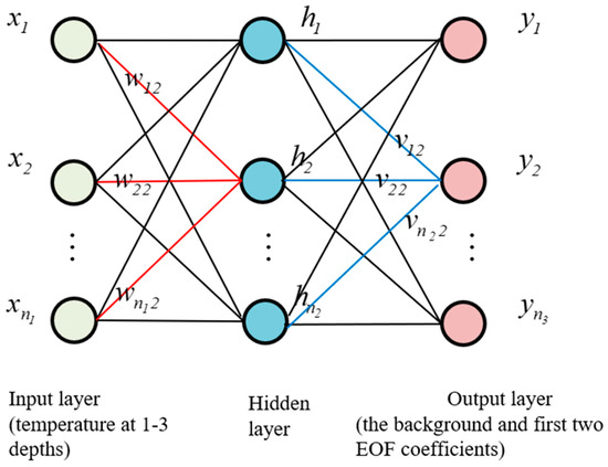
Figure 1.
Topological structure of BP network.
The learning process of the BP neural network can be divided into two stages: forward propagation and back propagation. The first is forward propagation, that is, the input data is passed in through the input layer, processed through the hidden layer and then reaches the output layer, and the network calculation result is obtained. The loss function of Equation (7) can calculate the error between the network calculation result and the actual output. If the loss error exceeds the threshold, it will enter the back propagation stage. Backpropagation is to transfer the loss error to the input layer through the hidden layer in reverse, and distribute the error to all units of each layer equally, and correct the connection weights of each unit according to the gradient descent method. Forward and backpropagation is performed in a loop, so that the connection weights can be continuously adjusted until the loss error is within the threshold range.
where, is the network output and is the actual output.
3. Experimental Results
3.1. Experimental Data
The South China Sea, with a mean depth of 1212 m, is obviously affected by the monsoon transition. Because of exchanging water with the adjacent seas through multiple straits, it has complex currents and an obvious multi-eddy structure. Therefore, the phenomena of internal waves are significant. The experimental data were measured by the Institute of Acoustics of the Chinese Academy of Sciences in the South China Sea in the autumn of 2015. Three thermistor chains composed of temperature-depth sensors (TD) were installed at H1 (114.63°E, 20.73°N), O1 (114.57°E, 20.71°N) and S17 (114.65°E, 20.60°N), respectively, as shown in Figure 2.
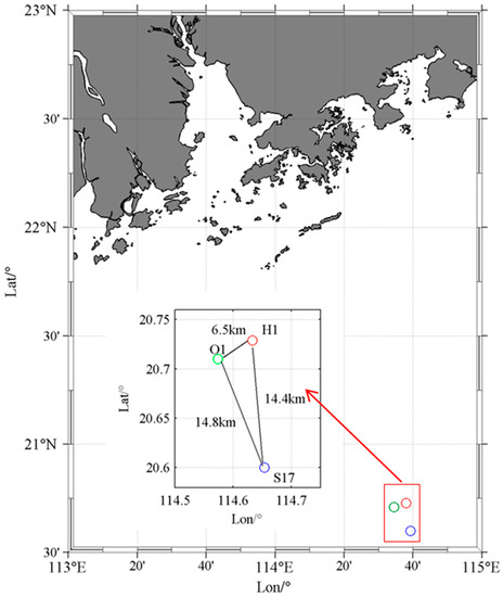
Figure 2.
Location distributions of the three thermistor chains.
As we can see from Figure 3, the temperatures recorded by thermistor chains at the three stations change with depth and time. The internal solitary waves accompanied by internal tides are obvious. The thermocline fluctuates greatly, and its depth is mostly in the range 25 m–75 m. Before building a neural network, data classification must be performed first, that is, the experimental data is divided into training set and test set. The solid white box in Figure 3a is the selected experimental data, of which 401 temperature profiles within the dotted white box are the test set, and the rest of the 1050 temperature profiles are the training set.
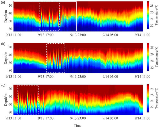
Figure 3.
The whole temperature profiles from 13 September, 11:00 to 14 September, 11:00 (GTM), recorded every 30 s. The data in the white dotted box is the test set, and the rest of the data in the white solid box is the training set. (a) H1, (b) O1, (c) S17.
The completeness of the training set is directly related to the training model’s performance. Therefore, two types of experimental data are selected for the training set. The first type of data are relatively stable temperature profiles observed at 11:00–16:00 on September 13, which can reflect the general trend of seawater temperature changes in the experimental area. The others are the temperature profiles with drastic fluctuation observed at 19:30–24:00 on 13 September, which can reflect transient characteristics of temperature profiles. The test set includes temperature profiles with sharp fluctuations under internal wave disturbance, so it can be used to evaluate the generalization ability of the trained model. In addition, in order to verify whether the network model established by the training set of the H1 site is also applicable to its surrounding area, temperature data were also selected from the O1 and S17 sites (denoted by the dotted white box in Figure 3b,c, all containing 401 temperature profiles) as the test set.
3.2. EOF Decomposition
Usually, the mean temperature profile and EOF modes can be extracted from the training set. If the real-time EOF coefficients can be inverted, the temperature profiles can be estimated by Equation (6). However, the classical EOF method is suitable for the steady-state environment. As shown in Equation (4), the spatial characteristics of temperature disturbance are obtained through SVD. However, when there are internal waves, especially internal solitary waves, the background field will change greatly in a short time. At this time, if the temperature profile is reconstructed using Equation (6), significant error of the background field will be caused. Therefore, this paper proposes an orthogonal representation of the temperature profiles, considering the variation of the background field. Different from Equation (4), this paper directly performs SVD on the temperature matrix T:
The component with the most significant contribution represents the background field, which could decompose to be the background field coefficient and background field mode. Since the cumulative contribution rate of the first two EOF modes exceeds 95%, the temperature profiles are reconstructed using the first two EOF modes, and the ith temperature profile can be approximately expressed as:
where represents the background field coefficient, and represents the background field mode.
Figure 4 shows the background field modes and the first two EOF modes extracted from the training set and the test set of H1, respectively. The background field mode extracted from the training set is highly consistent with the mean temperature profile of the training set. This is because the background field reflects the variation of temperature profiles in the steady-state environment, which approximates the mean temperature profile. It is quite different from the background field mode extracted from the test set, which indicates that the temperature field changes significantly in a short time, as shown in Figure 4a. Figure 4b,c show that these two EOF modes of different data sets are highly correlated with correlation coefficients of 0.99 and 0.92, respectively. For the training set, the first EOF mode has an extreme point, corresponding to a depth of z1 = 56 m, and it is found that the temperature of each temperature profile at this depth reflects the vertical displacement of the thermocline. The second EOF mode has four extreme points. According to the physical meaning of the first two EOFs, it is considered that the two extreme points near z1 represent the upper and lower bounds of the thermocline, and their corresponding depths are z2 = 50 m and z3 = 63 m. This will be explained in detail in Section 3.3.
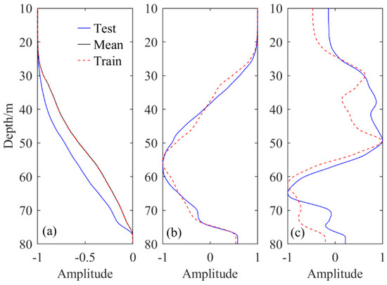
Figure 4.
Normalized background field modes and first two EOF modes, (a) The background field modes extracted from the training set and the test set and the normalized mean temperature profile of the training set, (b) the first EOF modes from the training set and the test set, (c) the second EOF modes extracted from the training set and test set.
3.3. Analysis of EOF Coefficients
3.3.1. Physical Meaning of the First Two EOF Coefficients
Casagrande et al. [18] explained the physical interpretation of the EOF coefficients. It was shown that the first EOF coefficient represents the vertical displacement of the thermocline, and the larger value means the shallower thermocline. The second EOF coefficient represents the change of the temperature gradient, and the larger value means a higher variable thermocline. Figure 4b shows the depth corresponding to the extreme point of the first EOF mode is z1 = 56 m, and Figure 4a shows the mean temperature is at 56 m. Figure 5a shows the normalized 24 °C isotherm of the temperature profiles and the normalized first EOF coefficient in the training set. It shows that these two parameters are highly correlated, and the correlation coefficient is 0.98 approximately. Figure 6a plots the depth of the 24 °C isotherm versus the first EOF coefficient. The fitted line shows that these two parameters are strongly linearly dependent; is the depth corresponding to the 24 °C isotherm. This shows that the first EOF coefficient can approximately reflect the depth of the thermocline. The temperature gradient of the training set between z2 and z3 is calculated. Figure 5b shows the normalized temperature gradient and the normalized second EOF coefficient. It can be seen that they are highly correlated and the correlation coefficient reaches 0.90. The fitted line in Figure 6b shows that the second EOF coefficient depends on the temperature gradient between z2 and z3. The fitted line of Figure 6b can be represented:
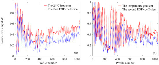
Figure 5.
Normalized amplitudes of the first two EOF coefficients, isotherm, and temperature gradient. (a) The normalized first EOF coefficient and the normalized 24 °C isotherm, (b) the normalized second EOF coefficient and the normalized temperature gradient.
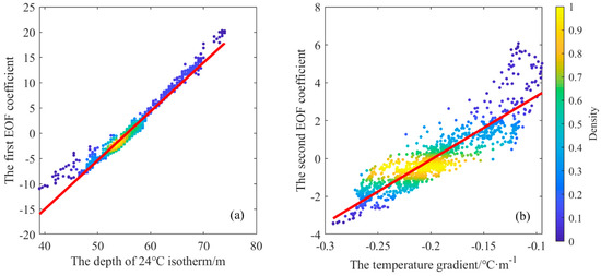
Figure 6.
Correlation analysis of the first two EOF coefficients with the isotherm and the temperature gradient. (a) The scatter diagram and fitted line of the first EOF coefficient and the 24 °C isotherm, (b) the scatter diagram and fitted line of the second EOF coefficient and the temperature gradient.
The above results show that if the temperatures at the depth z2 and z3 are measured, the second EOF coefficient can be derived from the temperature gradient using a linear relationship. The above analysis provides a reference for the selection of the depth-fixed temperature.
3.3.2. Correlation Analysis of the EOF Coefficients
The statistical relationships between the background field coefficient and the first two EOF coefficients in the internal wave environment are deeply analyzed. Figure 7a draws the background field coefficient versus the first EOF coefficient, and the red line represents the linear fit to the cloud of points. It shows that there is an obvious linear correlation between these parameters. Figure 7b plots the first EOF coefficient versus the second EOF coefficient, and the red curve represents the quadratic fit to the cloud of points. It illustrates that despite the orthonormal constraints of the EOF analysis, the first two modes are dynamically linked. Figure 7 shows that if the second EOF coefficient is known, the background field coefficient and the first EOF coefficient can be derived through these correlations.
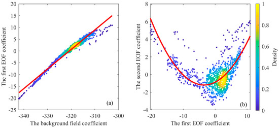
Figure 7.
Statistical characteristics of background field coefficient and the first two EOF coefficients. (a) The scatter diagram and fitted line of the background field coefficient and the first EOF coefficient, (b) the scatter diagram and fitting curve of the first EOF coefficient and the second EOF coefficient.
Combined with the conclusion in Section 3.3.1, if the temperatures at the depths and are known, the coefficients in Equation (9) can be deduced, and the temperature profiles can be inverted by combining the EOF modes extracted from the training set. However, the relationship between these parameters can only be roughly represented by the polynomial fitting method, and a complex mathematical model cannot be fitted. The BP neural network can capture the relationship between the temperature at the depths , and the EOF coefficients with its excellent nonlinear mapping ability, so as to achieve higher precision inversion.
4. Temperature Profile Inversion and Analysis
The analysis in Section 3.3 shows that the temperature profile has significant differences at various depths, and the thermocline has the largest disturbance (information). Thus the thermocline information can be used to reconstruct the whole profile to a large extent. By analyzing the statistical relationship between the vertical displacement, the gradient of thermocline and the first two EOF coefficients, it can be seen that when the sampling point is set at the critical depth, the reconstruction accuracy of the whole profile can be effectively improved. The temperature inversion results are analyzed in detail in this section.
4.1. Inversion of Temperature Profiles at H1
The emergence of marine mobile observation platforms makes it possible to obtain depth-fixed data. How to invert the full-depth temperature profiles with high precision through the minimum depth-fixed temperatures is the focus of this paper. The BP neural network has excellent multi-dimensional function mapping ability and can approximate any continuous function to realize the mapping between any dimensions. Therefore, the BP network can be used to establish the complex relationship between these depth-fixed temperatures and the background field coefficient, and the first two EOF coefficients. Then the temperature profiles can be inverted by combining the background field mode and the first two EOF modes which are extracted from the training set.
Configuring the best network parameters is the key to obtain the optimal network training model. For BP neural network, it is critical to select the number of hidden layers. Figure 8 depicts the normalized root mean square error (RMSE) calculated by Equation (11) of temperature inversion and the normalized model training time with the number of hidden layers. It can be seen that too low a number of hidden layers will cause too large an RMSE; and too many hidden layers will make the network training take too long. When the hidden layer is set to three layers, the balance between accuracy and efficiency can be achieved. In addition to the number of hidden layers, it is necessary to set the number of training times, learning rate and minimum error of training target. The experimental results show that when the number of hidden layers is 3, the learning rate is 0.01, the number of training is 1000, the minimum error of the training target is 10−4 and the gradient descent method is used to train, a more reliable training model can be obtained.
where is the RMSE of the kth temperature profile, and are the inversion temperature and actual temperature of the kth profile at the depth respectively, and N is the number of depth points.
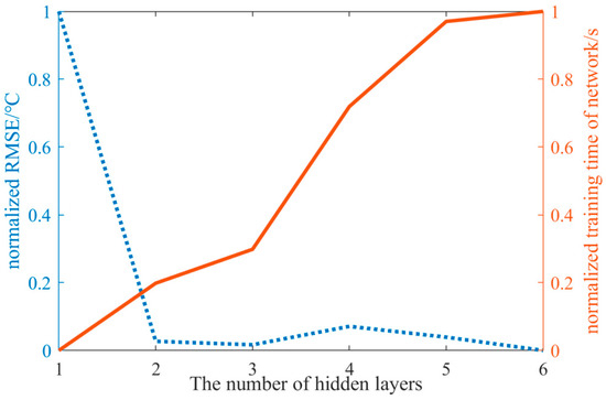
Figure 8.
The normalized root mean square error (RMSE) of temperature profile inversion and the normalized model training time with the number of hidden layers.
The selection of the depth of the depth-fixed temperature is directly related to the applicability of the training model and the accuracy of the inversion results. Taking the 401 temperature profiles in the test set at H1 as an example, the mean RMSE of full-depth temperature profiles reconstructed from temperature at a certain depth which is normalized is shown in Figure 9. The red line is the normalized first EOF; the blue line is the normalized absolute value of the second EOF, and the three gray dotted lines represent the depths z1, z2, z3, respectively. For the convenience of comparison, we normalized all three curves. It shows that the mean RMSE decreases first and then increases with the increase of the measurement depth. When the measurement depth is between z2 and z3, the mean RMSE is basically unchanged and reaches the minimum value. Combined with the analysis in Section 3, we attribute this phenomenon to the fact that this range contains the depth of the extreme point of the first two EOF basis functions, and the temperature at this depth can almost reflect all the information of the thermocline.
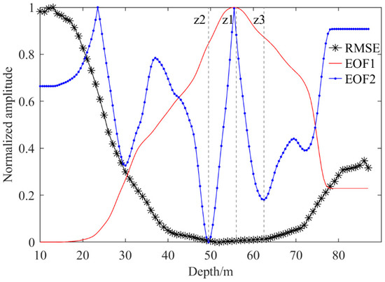
Figure 9.
Mean RMSE of test set temperature profiles reconstructed from temperatures at a certain depth (denoted as black stars). The red line is the normalized first EOF; the blue line is the normalized absolute value of the second EOF, and the three gray dotted lines represents the depth z1, z2, z3, respectively.
In order to show the effect of the depth of the depth-fixed temperature on inversion accuracy in detail, several representative cases (depth-fixed temperatures at 10 m, 50 m, 56 m and 63 m) were selected for analysis. The temperature at 10 m is taken because it is the shallowest depth of the thermistor chain. This temperature can be considered as the sea surface temperature, which could be easily obtained by a surface velocimeter. The surface velocimeter is usually fixedly installed on autonomous navigation platforms such as ships and submarines to obtain sea surface data. If the measured data of the surface velocimeter is available, the surface temperature is replaced by the actual measured value. Since the sea surface temperature is the most easily obtained depth-fixed temperature data, the temperature profile of the test set was firstly reconstructed using only the sea surface temperature. 56 m is the corresponding extreme point of the first EOF mode in the training set; 50 m and 63 m are the depths corresponding to the extreme points of the second EOF mode in the training set. With the development of marine mobile platforms, AUVs and other underwater vehicles can obtain depth-fixed temperatures in real-time through depth control. It was shown that the AUVs can achieve depth tracking with steady-state error in decimeters or even centimeters [21,22]. The temperature profile variation within the error range can be ignored. Hence, the temperatures at fixed depth are simulated by the temperatures of the thermistor chain at this depth.
The mean RMSE and standard RMSE of the temperature inversion in the test set is calculated by Equations (11) and (12), as shown in Figure 10. It can be seen that the depth selection of the depth-fixed temperatures has a great influence on the temperature profile inversion. The shallowest temperature has the lowest inversion accuracy, and the inversion results are the most unstable. For the other three depths, most of the inversion errors are very low. The mean RMSE in the test set is about 0.13 °C, and the standard deviation is about 0.035 °C. The reason is that 50 m and 63 m are the average depths of the upper and lower bounds of the thermocline, respectively. The temperature at 56 m can reflect the vertical displacement of the thermocline, and the temperature profile mainly depends on the characteristics of the thermocline.
where is the mean error of all profiles, is the standard deviation of all profiles, and n is the number of profiles.
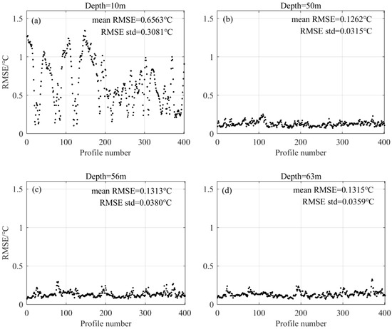
Figure 10.
The influence of temperature at different depths as the input data on the inversion results. The depths of (a–d) are 10 m, 50 m, 56 m, 63 m, respectively.
It is conceivable that with the increase of the input information, the inversion accuracy of the temperature profiles will be improved. Thus, we try to use two or three depth-fixed temperatures as input. As shown in Figure 11, the RMSE of the temperature profile inversion is basically reduced to 0.2 °C. Compared with the inversion results using one depth-fixed temperature as input, the accuracy is significantly improved. When the input data are the temperatures at the extreme point of the first two EOF basis functions, the inversion accuracy is the highest. The mean RMSE in the test set is about 0.11 °C, and the standard deviation is about 0.025 °C.
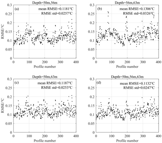
Figure 11.
The mean RMSE of inversion temperature profiles by temperatures at depths of 50, 56 m and 63 m. The depths of the input temperatures are (a) 50 m and 56 m, (b) 56 m and 63 m, (c) 50 m and 63 m, (d) 50 m, 56 m and 63 m.
We may take Figure 11d as an example to draw the RMSE of each temperature profile in depth, as shown in Figure 12. It can be seen that the temperature inversion error is the largest in the range of the thermocline (except the selected depths). This is because the internal waves cause the temperature profiles to change instantaneously and rapidly at the thermocline. The temperature field can be expressed as a random process consisting of the large-scale background and small-scale dynamic changes. The large-scale background changes mainly depend on the seasonal background temperature field. The small-scale dynamic changes usually refer to a spatially localized contribution from linear and non-linear internal waves. The background field has strong seasonal regularity, so its characteristics are easily captured. However, the small-scale dynamic processes such as internal waves change dramatically in the thermocline; in particular, the solitary internal wave has a certain randomness, so it is difficult to predict. Therefore, even if the temperature data at the depth of the first two EOF extreme points are input as a limiting condition, this can only reduce the sea temperature prediction error in the thermocline, but it cannot eliminate this error. Therefore, the temperature prediction error is still a little significant at a depth of 30–50 m.
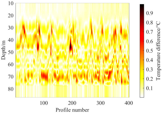
Figure 12.
The RMSE of inversion temperature profiles by temperatures at depths of 50, 56 m and 63 m.
4.2. Temperature Profiles Inversion at O1 and S17
In order to verify the spatial applicability of the training model, this paper also selects temperature profiles from the O1 and S17 sites as the test set. Figure 13a shows that the RMSE of the temperature inversion at the O1 is mostly below 0.2 °C except for 7 profiles. Figure 13b shows the mean RMSE of the temperature inversion at the S17 is slightly larger than that at the O1. The reason might be the fact that S17 is farther from H1 than O1. Therefore, the temperature profiles at S17 are more different from the profiles in the training set, which leads to a decrease in the accuracy.
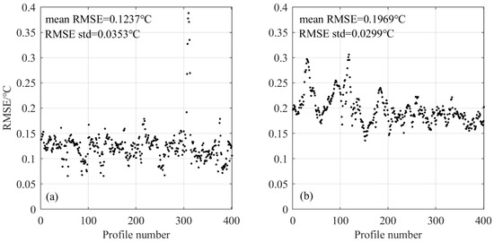
Figure 13.
The RMSE of temperature inversion at O1 and S17. (a) O1, (b) S17.
Figure 13a shows that 7 profiles have obvious larger errors, and the reason might be explained by Figure 14. The gray lines are the temperature profiles of the training set, the black lines are the 7 temperature profiles with obvious larger errors at the O1. The red dotted line is the mean temperature profile of the training set, as shown in Figure 14. It can be seen that these 7 profiles fluctuate drastically compared with the mean temperature profile, and the training set does not contain this type of temperature profiles. These two reasons mean that the inversion accuracy of these 7 profiles is poor.
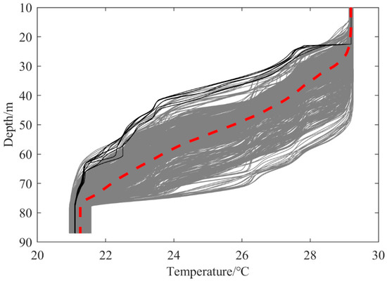
Figure 14.
Temperature profiles in the training set and some temperature profiles with large errors in the test set.
5. Conclusions
(1) Based on the measured temperature data in the South China Sea, the intrinsic statistical relationship between the background field coefficient and the first two EOF coefficients is deeply explored. According to the variation trend between the first two EOF coefficients and the depth and gradient of the thermocline, the physical meaning of the depth of the first two EOF basis functions is obtained.
(2) With the excellent nonlinear mapping ability of the BP neural network, the model for reconstructing the full-depth temperature profile using a few temperatures at fixed depth is established. The temperatures at three extreme points of the first two EOF modes, which can almost reflect all the information of the thermocline, are selected as the input, and the data of three thermocline chains from different stations are used to verify the training network. The results show that the inversed temperature profile is in good agreement with the measured values. The mean RMSE of the temperature profiles at the same station as the training set is about 0.1 °C, and the mean RMSE of the temperature profiles at the other two stations is about 0.2 °C.
6. Discussion
The nonlinearity and uncertainties of the marine vehicle model, and environmental disturbances create challenges for the practical application of the depth tracking design. However, with the development of marine mobile platforms, AUVs and other underwater vehicles can obtain depth-fixed temperatures in real-time through depth control. It is shown that the AUVs can achieve depth tracking with steady-state error in decimeters or even centimeters; the temperature profile variation within the error range can be ignored. Due to the lack of depth-fixed measurement temperatures, the temperatures at fixed depth are simulated by the temperatures of the thermistor chain at this depth. If data measured by the underwater vehicles are available, the depth-fixed temperatures could be replaced by the actual measured values.
Based on the back propagation (BP) neural network, this paper reconstructs the full-depth temperature profile using a few temperatures at fixed depth. Compared with the traditional observation by anchoring a thermistor chain, this method is flexible and autonomous. However, the spatial adaptability of training networks generated from a fixed station needs to be further studied.
Author Contributions
Conceptualization, Q.L.; methodology, Q.L. and X.Y; software, X.Y.; validation, Q.L., X.Y., Z.W., Z.L., S.C. and Q.T.; writing—original draft preparation, X.Y.; writing—review and editing, Q.L. and X.Y. All authors have read and agreed to the published version of the manuscript.
Funding
This research was funded by the Natural Science Foundation of Shandong Province of China (Grant ZR2022MA051 and ZR2020MA090), The National Natural Science Foundation of China under contract (Grant U22A2012), China Postdoctoral Science Foundation (Grant 2020M670891), the SDUST Research Fund (Grant 2019TDJH103), and the Talent Introduction Plan for Youth Innovation Team in universities of Shandong Province (innovation team of satellite positioning and navigation).
Data Availability Statement
The datasets used in this study were measured by the Institute of Acoustics of the Chinese Academy of Sciences in the South China Sea in the autumn of 2015.
Conflicts of Interest
The authors declare no conflict of interest.
References
- Sun, D.J.; Yu, M.; Cai, K.J. Inversion of ocean sound speed profiles from travel time measurements using a ray-gradient-enhanced surrogate model. Remote Sens. Lett. 2022, 13, 888–897. [Google Scholar] [CrossRef]
- Li, B.Y.; Zhai, J.S. A Novel Sound Speed Profile Prediction Method Based on the Convolutional Long-Short Term Memory Network. J. Mar. Sci. Eng. 2022, 10, 572. [Google Scholar] [CrossRef]
- Li, H.P.; Qu, K.; Zhou, J.B. Reconstructing sound speed profile from remote sensing data: Nonlinear inversion based on Self-Organizing Map. IEEE Access 2021, 9, 109754–109762. [Google Scholar] [CrossRef]
- Rubenstein, D. Observations of cnoidal internal waves and their effect on acoustic propagation in shallow water. IEEE J. Ocean. Eng. 1999, 24, 346–357. [Google Scholar] [CrossRef]
- Lv, Z.C.; Du, L.B.; Li, H.M.; Wang, L.; Qin, J.X.; Yang, M.; Ren, C. Influence of Temporal and Spatial Fluctuations of the Shallow Sea Acoustic Field on Underwater Acoustic Communication. Sensors 2022, 22, 5795. [Google Scholar] [CrossRef]
- Khan, S.; Song, Y.; Huang, J.; Piao, S. Analysis of underwater acoustic propagation under the influence of mesoscale ocean vortices. J. Mar. Sci. Eng. 2021, 9, 799. [Google Scholar] [CrossRef]
- Zhang, L.; Song, Y.; Zhou, S.D.; Liu, F.; Han, Y. Review of measurement techniques for temperature, salinity and depth profile of sea water. Mar. Sci. Bull. 2017, 36, 481–489. [Google Scholar]
- Hurlburt, H.E.; Fox, D.N.; Metzger, E.J. Statistical inference of weakly correlated subthermocline fields from satellite altimeter data. J. Geophys. Res. Oceans 1990, 95, 11375–11409. [Google Scholar] [CrossRef]
- Guinehut, S.; Traon, L.; Larnicol, G.; Philipps, S. Combining Argo and remote- sensing data to estimate the ocean three-dimensional temperature fields-a first approach based on simulated observations. J. Mar. Syst. 2004, 46, 85–98. [Google Scholar] [CrossRef]
- Han, Z.; Zhao, N. Seawater temperature model from Argo data by LM-BP neural network in Northwest Pacific Ocean. Mar. Environ. Sci. 2012, 31, 555–560. [Google Scholar]
- Munk, W.; Wunsch, C. Ocean acoustic tomography: A scheme for large scale monitoring. Deep Sea Research Part A. Oceanogr. Res. Pap. 1979, 26, 123–161. [Google Scholar] [CrossRef]
- Munk, W.H.; Worcester, P.; Wuncsh, C. Ocean Acoustic Tomography; Cambridge University Press: Cambridge, UK, 1995. [Google Scholar]
- Shang, E.C. Ocean acoustic tomography based on adiabatic mode theory. J. Acoust. Soc. Am. 1989, 85, 1531–1537. [Google Scholar] [CrossRef]
- Tolstoy, I.A. Low-frequency acoustic tomography using matched field processing. J. Acoust. Soc. Am. 1989, 86, S7. [Google Scholar] [CrossRef]
- Zhang, Z.; Li, Z.; Dai, Q. Sound speed profile reconstruction from the data measured in a limited depth. Technol. Acoust. 2008, 27, 106–107. [Google Scholar]
- Taroudakis, M.; Papadakis, J. A modal inversion scheme for ocean acoustic tomography. J. Comp. Acoust. 1993, 1, 395–421. [Google Scholar] [CrossRef]
- Leblanc, L.; Middleton, F. An underwater acoustic sound velocity data model. J. Acoust. Soc. Am. 1980, 67, 2055–2062. [Google Scholar] [CrossRef]
- Casagrande, G.; Varnas, A.W.; Stephan, Y.; Thomas, F. Genesis of the coupling of internal wave modes in the Strait of Messina. J. Mar. Syst. 2009, 78, S191–S204. [Google Scholar] [CrossRef]
- Li, Q.; Shi, J.; Li, Z.; Luo, Y.; Yang, F.; Zhang, K. Acoustic sound speed profile inversion based on orthogonal matching pursuit. Acta Oceanol. Sin. 2019, 38, 149–157. [Google Scholar] [CrossRef]
- Rumelhart, D.E.; Hinton, G.E.; Williams, R.J. Learning representations by back-propagating errors. Nature 1986, 323, 6088. [Google Scholar] [CrossRef]
- Liu, C.; Xiang, X.; Yang, L.; Li, J.; Yang, S. A hierarchical disturbance rejection depth tracking control of underactuated AUV with experimental verification. Ocean Eng. 2022, 264, 112458. [Google Scholar] [CrossRef]
- Tanakitkorn, K.; Wilson, P.A.; Turnock, S.R.; Phillips, A.B. Depth control for an over-actuated, hover-capable autonomous underwater vehicle with experimental verification. Mechatronics 2017, 41, 67–81. [Google Scholar] [CrossRef]
Publisher’s Note: MDPI stays neutral with regard to jurisdictional claims in published maps and institutional affiliations. |
© 2022 by the authors. Licensee MDPI, Basel, Switzerland. This article is an open access article distributed under the terms and conditions of the Creative Commons Attribution (CC BY) license (https://creativecommons.org/licenses/by/4.0/).