Modeling and Analysis of Microwave Emission from Multiscale Soil Surfaces Using AIEM Model

Abstract

Natural rough surfaces have inherent multiscale roughness. This article presents the modeling and analysis of microwave emission from a multiscale soil surface. Unlike the linear superposition of different correlation functions with various correlation lengths, we applied the frequency modulation concept to characterize the multiscale roughness, in which the modulation does not destroy the surface’s curvature but only modifies it. The multiscale effect on emission under different observation geometries and surface parameters was examined using an AIEM model. The paper provides new insights into the dependence of polarized emissivity on multiscale roughness: V-polarized emissivity is much less sensitive to multiscale roughness across the moisture content from dry to wet (5–30%). The H-polarized is sensitive to multiscale roughness, especially at higher moisture content. The predicted emissivity will have considerable uncertainty, even for the same baseline correlation length, without accounting for the multiscale roughness effect. V-polarized emissivity is less sensitive to the multiscale effect than H-polarized and the higher modulation ratio indicates larger emissivity. The higher modulation ratio indicates larger emissivity. Multiscale roughness weakens the polarization difference, particularly in higher moisture conditions. In addition, ignoring the multiscale effect leads to underestimated emissivity to a certain extent, particularly at the larger RMS height region. Finally, when accounting for multiscale roughness, model predictions of emission from a soil surface are in good agreement with two independently measured data sets.

1. Introduction

Many parameters control the roughness variation in the formation process of the soil surface, resulting in multiscale roughness, ranging from topographic to microstructure scales. In terms of the autocovariance function, spatial short-range and long-range correlations exist. The soil surface’s scale-dependent roughness variations have been documented in [1,2]. Reasonable attempts have been made to model the sources of spatial variations by fractal and non-fractal approaches. In the context of modeling microwave scattering from the soil surface, how the sensor responds to multiscale roughness of the soil surface has been studied in considerable detail [3,4,5,6,7,8,9,10,11,12,13]. Most of these studies have been mainly concerned with the influence of roughness on retrieving soil moisture from radar measurements. Two models predict accurate polarized scattering coefficients and emissivity. One is the electromagnetic scattering or emission model and the other is the surface model that characterizes the target surface’s geometrical (or statistical) and dielectric properties. These two issues are usually confused and intertwined.

Chen et al. [3] applied the frequency modulation concept to model multiscale roughness. The modulation process effectively changes the surface slope and shifts the peak location of roughness spectra. The study concluded that the effective correlation length should be defined and the normal incidence has to be reinterpreted. Mattia et al. [4] applied random fractals to describe the multiscale roughness of a soil surface. By adjusting the exponents of the power-law-like roughness spectrum, they could better match the backscattering coefficient between the EM model and numerical and experimental data. Research on multifractals to model the soil surface for radar backscattering with satisfactory results has been reported in [5,6,7].

It is generally accepted that the two-scale model [14] recovers the measured scattering data to a reasonable extent. Plant [15] considered a three-scale radar backscatter model from the sea. The waves were divided into small-, intermediate- and large-scale waves, where the small and intermediate scales were tilted, advected and modulated by large-scale waves. Then the Bragg resonant and Kirchhoff theories were applied to the respective region. The proposed model could accurately explain most features of the measured data, including the level and wind dependence of the nadir backscatter and the wind and azimuth angle dependence of the radar backscatter.

However, in terms of parameter estimation from radar measurement, the cut-off boundary of the various scales from large to small is not set systematically but heuristically. More recently, a multiscale roughness model was proposed [16] to estimate surface roughness at different spatial scales using proxy variables to improve the soil moisture from radiometer observations. The authors accounted for the multiscale from microroughness to topographic roughness at the spatial resolution of 1.5 and 3.0 km and this could be extended to other resolutions [16]. The roughness model was dependent on several soil parameters and land covers. The previous studies have made significant progress toward understanding the multiscale effects on both active and passive microwave observations; however, the distinction between small roughness and large roughness has not been fully justified on a physics basis to date. The coupling of generating and degenerating among various scales has made it even more difficult to delineate the roughness scales in the sense of probing wavelength. For the surface to be multiscale, how the individual scales play and interplay with the other scales to contribute to the scattering and emission remains to be explored.

A recent study [17] demonstrated that the modulation concept offers higher flexibility in modeling the radar scattering of a multiscale rough surface. The modulation concept stems from observing the oscillatory correlation function that exhibits zero-crossings in the stochastic process of random surfaces. The number of zero-crossings and their intervals in the correlation function may quantify different manifestations of multiscale signatures. The sources of such zero-crossings may also come from estimating the correlation function if the size of the rough surface is not sufficiently large. Adjusting the modulation ratio can account for the multiscale roughness effects. The results were validated by comparing backscattering coefficients from soil and sea-ice surfaces. By extending the work of [17], this paper aims to improve the understanding of the frequency response of microwave emission to multiscale roughness.

Before moving to the next section, it is worth mentioning that the objective of this paper is to account for the uncertainty in rough soil surface description, namely the multiscale property and its influence on microwave emission. On a global scale and on many natural surfaces, the vegetative canopy is a significant emission source when soil moisture content is of major interest. The microwave polarization difference index (MPDI) introduced in [18,19] was sensitive to the moisture content of the soil surface at 6.6 GHz and was a good indicator of the canopy parameters at a higher frequency, e.g., 37 GHz [18,19]. A theoretical derivation of MPDI was derived based on solving the zero-order radiative transfer model to account for the vegetation optical depth, which contributes to the total observed brightness temperature via a microwave radiometer [20]. It would be very interesting to investigate whether the concept of the MPDI can effectively reduce the influence of the multiscale roughness effect and include an MPDI when considering a vegetative soil surface in a future study.

2. Materials and Methods

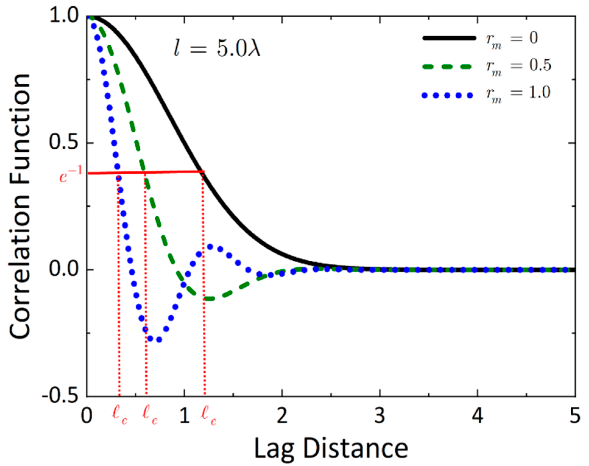
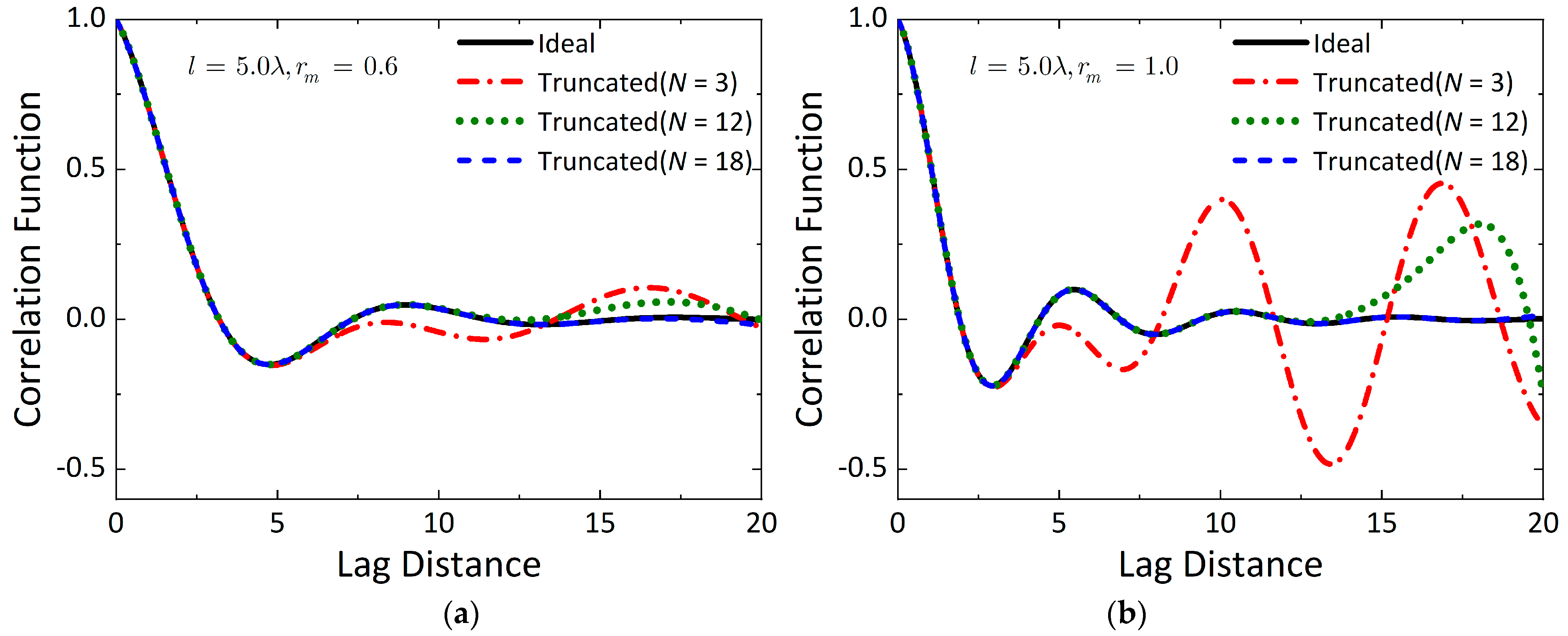
2.1. Multiscale Rough Surface: Decomposition of Multiscale Correlation Function

Bragg resonance is likely to occur among electromagnetic waves and various roughness scales when the electromagnetic waves are emitted from or through a rough surface. Hence, the multiscale effect will modify the behavior of the microwave emission. Figure 1 illustrates the multiscale roughness components of a rough surface profile: the different colored lines represent different roughness scales in terms of spatial wavenumber. To accurately predict the microwave emission, it is essential to have a surface model of a multiscale roughness surface to be incorporated into the emission model. From an analytical modeling point of view, the surface model requires statistical representation and is preferably mathematically manipulable.

Among several approaches, a multiscale rough surface can be modeled by modulating a single-scale surface with a modulation function [3,17]:

$${\rho }_m(r)=\rho (r)J_0\left(\frac{2\pi }{{\lambda }_m}\left|r\right|\right)$$

(1)

where $J_0(\cdot )$ is the zero-order Bessel function, ${\lambda }_m$ is the modulation length, $r=(r_x,r_y)$ is the lag distance in $x,y$ directions and $\rho (r)$ is the baseband correlation function of a single-scale surface. To model the roughness scale, we can define the modulation ratio as the correlation length, $l$ and the modulation length, ${\lambda }_m$:

$$r_m=l/{\lambda }_m.$$

(2)

In Equation (2), a larger $r_m$ involves more scales of roughness and $r_m=0$ reduces to a single-scale surface.

In Figure 2, we have plotted the Gaussian-modulated correlation function, ${\rho }_m(r)$, with different modulation ratios, $r_m=0, 0.5, 1.0$. Here, we consider the surface is isotropic with the correlation length set to ${\ell }_x={\ell }_y=\ell =5\lambda$. The black line denotes the Gaussian correlation function. Note that an effective correlation length, ${\ell }_e$, is defined by ${\rho }_m({\ell }_e)=e^{-1}$ and is dependent on the modulating wave number, whose value cannot be arbitrary without limits for a given multiscale surface [17].

To examine the surface continuity of Equation (1), we have computed the RMS slope by a second derivative of the correlation function evaluated at zero. For a Gaussian-modulated surface, we have

$$s=\sqrt{-{\frac{d^2{C}_m\left(r\right)}{d{r}^2}|}_{r=0}}=\sqrt{2}\frac{\sigma }{l}\sqrt{\left(1+{\pi }^2{r}_m^2\right)}$$

(3)

where we readily see that, when $r_m=0$, the RMS slope is reduced to a well-known result,$s=\sqrt{2}\frac{\sigma }{l}$ [14]. The term $\sqrt{\left(1+{\pi }^2{r}_m^2\right)}$ is the modulation factor of the RMS slope for a Gaussian-modulated surface.

Before proceeding, it would be interesting to know whether a curvature exists that is related to the fourth derivative of the correlation function evaluated at zero:

$$\gamma =\sqrt{{\frac{d^4{C}_m\left(r\right)}{d{r}^4}|}_{r=0}}=\sqrt{12}\frac{{\sigma }^2}{l^4}\sqrt{1+2{\pi }^2{r}_m^2+\frac{1}{2}{\pi }^4{r}_m^4}.$$

(4)

Equation (4) proves that the modulated surface, as given in Equation (1), does not destroy the surface’s curvature but only modifies it. It should be noted at this point that Equation (4) is only related to the average radius of curvature. To mathematically express the average radius of curvature, we need to know the probability density function of the variance of the surface’s second derivative. The derivation is beyond the scope of this study but deserves a future study.

We have plotted the RMS slope as a function of the modulation ratio, $r_m$ in Figure 3. Note that the RMS slope increases as the modulation ratio, $r_m$, increases. $r_m=0$ corresponds to the RMS slope of the Gaussian-correlated surface. When, $r_m=1$, we can see that the RMS slope of the Gaussian-modulated surface is 3.2 times that of the Gaussian surface.

By applying Taylor’s expansion of $J_0(\cdot )$ appearing in Equation (1), we can decompose a continuous multiscale correlation function into N ($N\to \infty$) roughness scales:

$${\rho }_m(r)=\underset{N\to \infty }{\lim }\frac{1}{N}\rho (r){\displaystyle \sum _{i=1}^N\left[J_0\left(\tilde{r}\right)+N{a}_i{J}_i\left(\tilde{r}\right)\right]}$$

(5)

with the weights

$$a_i=\frac{1}{i!}{\left(-1\right)}^i{\left(\frac{\tilde{r}}{2}\right)}^i$$

(6)

where $\tilde{r}=\frac{k_m\left|r\right|}{\sqrt{2}}$; $k_m=2\pi /{\lambda }_m$ is the modulation wave number; $\rho (r)$ is the correlation function of a single-scale surface; and $J_i(\cdot )$ is the i-order Bessel function.

When N is truncated to a certain number, being finite, we have the approximated correlation function, ${\widehat{\rho }}_m(r)$. The number of N required to make ${\widehat{\rho }}_m(r)$ converge to ${\rho }_m(r)$ depends on how oscillatory the modulated correlation function is: the more rapid the oscillation, the larger the N to approximate ${\widehat{\rho }}_m(r)$ to ${\rho }_m(r)$.

To illustrate the decomposition of a multiscale roughness, we have plotted the truncated ($N=3$) and the real ($N\to \infty$) correlation functions in Figure 4. Each of the three components are also shown. With $l=5.0\lambda$ and $r_m=0.4$, we find that $N=3$ is sufficient to represent a real ${\rho }_m(r)$. When increasing the modulation ratio, the correlation function exhibits more zero-crossings, namely more oscillatory, hence, requiring more terms in (5) to approximate the real ${\rho }_m(r)$ by the truncated ${\widehat{\rho }}_m(r)$, ${\rho }_m(r)\cong {\widehat{\rho }}_m(r)$. Figure 5a,b explain the cases of $r_m=0.6$ and $r_m=1.0$, respectively.

2.2. Computation of Microwave Emissivity Using AIEM Model

Microwave emissivity can be computed by:

$$\begin{array}{l}{e}_p=1-R_p\exp \left[-{\left(2k\sigma \cos {\theta }_i\right)}^2\right]\\ \hspace{1em}\hspace{1em}-\frac{1}{4\pi \cos {\theta }_i}{\displaystyle {\int }_0^{2\pi }{\displaystyle {\int }_0^{\pi }\left({\sigma }_{pp}^0+{\sigma }_{pq}^0\right)}}\sin {\theta }_{s}d{\theta }_{s}d{\varphi }_s\end{array}$$

(7)

where $R_p$ is the p-polarized Fresnel reflectivity and the pq-polarized bistatic scattering coefficients ${\sigma }_{pp}^0$ and ${\sigma }_{pq}^0$ under the AIEM model take the form:

$${\sigma }_{qp}^o=\frac{k^2}{2}{e}^{-{\sigma }^2\left(k_{sz}^2+k_z^2\right)}{\displaystyle \sum _{n=1}^{\infty }\frac{{\sigma }^{2n}}{n!}}{\left|{{\rm I}}_{qp}^n\right|}^2{\mathbf{W}}^{\left(n\right)}\left(k_{sx}-k_x,k_{sy}-k_y\right)$$

(8)

where ${\mathbf{W}}^{\left(n\right)}(\cdot )$ is the Fourier transform of the nth power of the modulated correlation function, ${\rho }_m$. Details of Equation (8) and its application to predicting microwave emission can be found in [21,22].

Extensive studies have dealt with the scattering for multiscale surfaces by linear superposition of different roughness scale components [23]. However, the linear superposition seems to ignore the interactions among different scales. That is to say, the scattering of multiscale rough surfaces may be underestimated or overestimated to an uncertain extent regarding the emission.

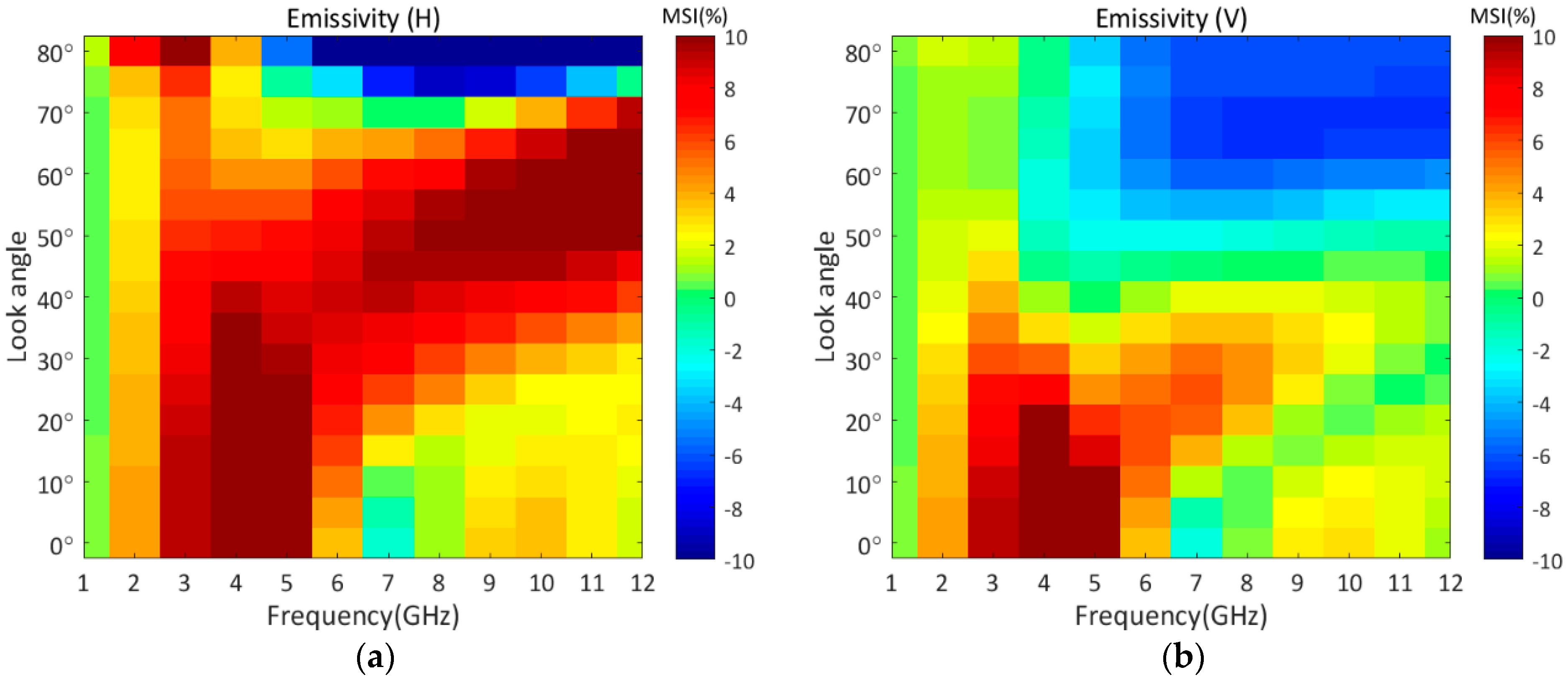
2.3. Multiscale Sensitivity Index (MSI)

To evaluate the influence of frequency and look angle on the multiscale sensitivity of emissivity, we can define a multiscale sensitivity index (MSI):

$$MSI=\frac{e_{p,m}-e_{p,um}}{e_{p,um}}$$

(9)

where $e_{p,m},e_{p,um}$ are the emissivities from the multiscale and single-scale rough surface at p polarization, respectively. In Equation (9), p- can be either H or V polarization. For $MSI$, a dimensionless quality index, $MSI= 0$ means that the multiscale effect has no effect, $MSI>0$ indicates that emissivity is enhanced by the multiscale effect and $MSI<0$ indicates that emissivity is diminished by the multiscale effect.

3. Results

Figure 6 illustrates a numerical simulation of backscattering from multiscale surfaces. As shown in Figure 6, we have plotted the backscattering with the analytical and combined correlation functions, which corresponds to the setup of Figure 4.

We note that the backscattering coefficients are overestimated when the linear superposition of three scales obtains a multiscale correlation function. This phenomenon is attributed to neglecting the interactions among different scales. Therefore, this study adopted an analytical modulation correlation function to demonstrate the scattering and emission for multiscale soil surfaces. From the contributions of backscattering at different scales, we can see that the difference in backscattering coefficients for different roughness scales is more pronounced at small incident angles.

3.1. Parameter Dependence

3.1.1. Influence of Frequency

Figure 7 plots the emissivity as a function of frequency (1~12 GHz). The exponential modulated multiscale surfaces were selected with the modulation ratio varying from 0 to 1. For numerical illustrations, we selected the look angle of 40° and the RMS height of 0.5 cm. The permittivity was set as 12 − j1.8. For the unmodulated rough surface ($r_m=0$), the baseband correlation length was fixed at 5cm. We calculated the emissivity with two effective correlation lengths, $l_e=1.92 \mathrm{cm} \left(r_m=0.6\right)$ and $l_e=1.25 \mathrm{cm} \left(r_m=1.0\right)$, for exponential modulated surfaces. From Figure 7a, both for H and V polarizations, the emissivities of unmodulated surfaces increase linearly with frequency. The difference between the H- and V-polarized emissivities decreases with frequency. In addition, a larger $r_m$ shrinks the polarization difference, especially at higher frequency regions (>9.6 GHz). In addition, as the frequency increases, the polarization diversity of the emissivity drops when finer scales of roughness are present. Moreover, the H-polarized emissivity is more sensitive to the multiscale effect.

To further investigate the polarization diversity of emissivity in frequency, Figure 7a displays the difference in emissivity between the H and V polarizations. The related parameters are the same as in Figure 7a. As a reference, we first examined the emissivity of an unmodulated rough surface ($r_m=0$), which is an exponential correlated surface. We can clearly see that the difference in emissivity for a modulated rough surface ($r_m=0.6,1.0$), compared to the unmodulated rough surface, decreases nonlinearly as the frequency increases. On the other hand, the difference between H- and V-polarized emissivities is more sensitive to the modulation ratio at the C band.

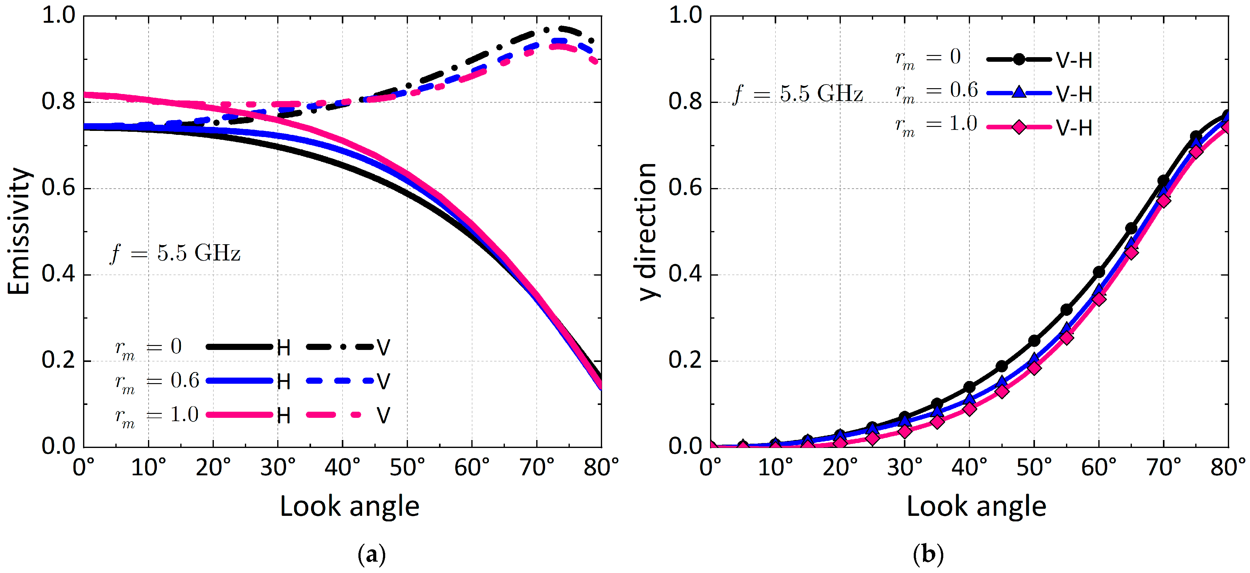
3.1.2. Influence of Look Angle

Next, we examined the influence of the look angle (0~80°) on the emissivity for unmodulated ($r_m=0$) and modulated ($r_m=0.6$) rough surfaces, as shown in Figure 8a. For numerical illustration, we set the frequency to 5.5 GHz, the RMS height to 0.5 cm and the permittivity to 12 − j1.8. By observing the emissivities from Figure 8a, we can see that both the H- and V-polarized emissivities, due to the modulation effect, are significantly enhanced at small and moderate look angles. This deviation may be attributed to the change in effective roughness at a small look angle. That is, if the multiscale effect is ignored, the emissivities are underestimated, especially at small and moderate look angles. In addition, as the modulation ratio increases, the V-polarized emissivity decreases slightly at large look angles.

We evaluated the polarization diversity of the emissivity at different look angles, as shown in Figure 8b. In general, the emissivity difference for the unmodulated surface is lower than that for the modulated surface. In addition, we can see that the emissivity difference is very small when the modulation ratios are 0.6 and 1.0, implying that the modulation ratio is not effective for polarization diversity. We can conclude that the polarization difference in emissivity is sensitive to multiscale effects to some extent. The polarization difference reaches saturation when the rough surface presents finer scales; in this case, the multiscale effect no longer acts effectively.

Figure 9 displays the MSI as a function of look angle and frequency with $l=5 \mathrm{cm}$, $r_m=0$. The emissivities of a multiscale surface were evaluated with a modulation ratio of 1.0. In addition, the RMS height was set to 0.5 cm and the relative permittivity was 12 − j1.8. From Figure 9, it can be seen that the dynamic range of the MSI is −10%~10%. Most notably, for H polarization, the greatest positive impact, in which the MSI is around 10%, is concentrated in the C band with small look angles (<30°) and in the X band with large look angles (50~70°). However, the greatest negative impact, with the MSI of around −10%, is located at the X band with larger look angles (>70°). The MSI is close to zero for V polarization at 45~50° incidence. These phenomena imply that the emissivity is much less sensitive to the multiscale effect at 45~50° for L, C and X bands. The results also confirm that the multiscale effect is negligible when measuring emissivity at 45~50° in V polarization.

3.2. Surface Parameter Dependence

3.2.1. Influence of Roughness

Recalling that the modulation ratio, $r_m$, describes different roughness scales, $r_m=0$ indicates an unmodulated rough surface with only a single correlation length. As $r_m$ increases, the rough surface presents more scales of roughness. In this case, the rough surface is multiscale, presenting small-scale roughness riding on large-scale roughness. Accordingly, the correlation length is changed by the modulation ratio. The effective correlation length decreases as the modulation ratio increases [17]. The modulation of different scales complicates the emissivity from such a rough surface.

To illustrate such an effect, as shown in Figure 10a, we examined the effect of the modulation ratio by varying it from 0 to 1.2. For the convenience of simulation, we chose 5.5 GHz (C band) as the sensor frequency at three look angles of 20°, 40° and 60°. The baseband correlation length was fixed at 5 cm and the RMS height was set to 0.5 cm. As shown in Figure 10a, the higher modulation ratio indicates a stronger emissivity for both H and V polarizations. This is because the effective roughness increases as the modulation ratio increases. We can also see that the change rate of emissivity depends on the look angle. For the look angle of 20°, the emissivity induced by the modulation increases more rapidly. This implies that the emissivity is more sensitive to the multiscale effect at the small look angle. Figure 10b plots the polarization difference in emissivity varying with the modulation ratio at three look angles. As the modulation ratio increases, the emissivity difference between H and V polarizations is weakened. It is also worth mentioning that the polarization difference in emissivity is less sensitive to multiscale effects at a small look angle.

We inspected the dependence of RMS height on emissivity, as shown in Figure 11a. By comparison, the results show that the trends of emissivity for H and V polarizations are quite different. From Figure 11a, we can see that as the RMS height increases, the emissivity increases and H-polarized emissivity increases faster. With the increased RMS height, the emissivity between single- and multiscale surfaces deviates. Compared to the single-scale surface, the emissivities at both H and V polarizations are enhanced due to the multiscale effect. The multiscale effect becomes more apparent when the RMS height is larger. Namely, if the multiscale effect is ignored, the emissivities at larger RMS height regions are underestimated to a certain extent. Figure 11b plots the difference in emissivity between H and V polarizations. We find that, as the RMS height increases, the differences in emissivity significantly decrease. This implies that the polarization feature dims at the large RMS height. Meanwhile, the polarization difference is weakened due to multiscale effects.

To examine the coupling effects of RMS height and modulation ratio, we have presented the emissivity pattern, varying with these two surface parameters simultaneously. In this case, for numerical illustration, the dynamic range of the RMS height is 0.1~1.0 cm and that of the modulation ratio is 0~1.2. The simulation is given at a look angle of 40° and 5.5 GHz for an exponential modulated multiscale rough surface. The surface parameters are $l=5 \mathrm{cm}$, $r_m=1.0 \left(l_e=1.25 \mathrm{cm}\right)$ and ${\epsilon }_r=12-j1.8$. Figure 12 shows that strong emission occurs at the larger RMS height and higher modulation ratio regions. As we noted before, the larger the modulation ratio, the smaller the effective correlation length and this implies that increased roughness enhances the emissivity. By comparison, the dynamic range of the emission at H polarization is larger than at V polarization. That is to say, the H-polarized emissivity is more sensitive to surface roughness.

3.2.2. Influence of Soil Moisture

We have plotted the emissivity as a function of soil moisture varying from 5% to 30% in Figure 13a. The carrier frequency was set to 5.5 GHz and the look angle was 40°. For the illustration, we set the baseband correlation length to 5 cm and the RMS height to 0.5 cm, with three modulation ratios of 0, 0.6 and 1.0.

As shown in Figure 13a, higher soil moisture generates smaller emissivity at both H and V polarization. Nevertheless, we can note that the dynamic range of the emissivity at H polarization, given rise to by the modulation ratio, is larger than that at V polarization. This implies that the V-polarized brightness temperature is less sensitive to the multiscale when the soil moisture changes. For a better visually inspection of the polarization feature, as shown in Figure 13b, we also present the difference in emissivity between V and H polarizations under the single and multiscale surfaces. We can see that the polarization difference is enhanced as the soil moisture increases. Furthermore, the increase in the polarization difference slows down due to the multiscale effect.

Figure 13 plots the H- and V-polarized emissivities and their difference at the degree of multiscale roughness (different r_m, with r_m = 0 indicating a single-scale roughness). Figure 13 provides new insights into the dependence of polarized emissivity on multiscale roughness. V-polarized emissivity is much less sensitive to multiscale roughness across moisture content from dry to wet (5–30%). H-polarized emissivity is sensitive to multiscale roughness, especially at a higher moisture content. Even for the same baseline correlation length, without accounting for the multiscale roughness effect, the predicted emissivity will have considerable uncertainty. As the multiscale roughness effect exercises different extents on the polarization, the MPDI [18,19,20] will also have a significant bias. We can conclude at this point that the multiscale effect weakens the polarization differences, particularly in large soil moisture regions.

For a more profound multiscale analysis, we examined the coupling effect of soil moisture and baseband surface slope, shown in Figure 14, by fixing the baseband correlation length at 5 cm and varying the RMS height from 0.1 to 1 cm. In this case, the baseband surface slope increases with the RMS height, varying from 0.02 to 0.2 cm. For numerical illustration, we chose 0.6 as the modulation ratio for exponential modulated rough surfaces. Hence, the effective surface slopes are from 0.052 to 0.52 for multiscale surfaces, including smooth and rough surfaces. By observing the MSI from Figure 14, we can see that the MSI remains positive over the different surface baseband slopes and soil moisture for H polarization. However, the MSI appears negative at small surface baseband slopes for V polarization. This indicates that emissivity is enhanced by the multiscale except for the very small slope when we change the surface roughness and soil moisture individually or together.

3.3. Comparison of Emissivity with Experimental Data

In this section, we compare the emission by model predictions with three independent measurement data sets: one is snow surface measured at L and C bands [24] and the other two are bare soil surface measured at L, C and X bands [25,26].

3.3.1. Measurements from Snow Surface

The brightness temperature measurements were collected from snow surfaces at L and C bands in V and H polarizations [24]. This experiment was carried out in the 2004/2005 Austral summer at Dome-C, called “DOMEX” within the SMOS program. As reported in [24], the snowpack was composed of a succession of soft layers of kinetic growth grains, alternating with harder layers of rounded grains. The real part of the dielectric constant was 1.4~1.85. The infrared surface temperature of the snow was around −25 °C and the surface roughness was minimal. Measurements over the incident angle of 20~80° were reported. From Figure 15, we note that, by setting the modulation ratio to 0.12, the model predictions at both V and H polarizations match the measurements well in the angular trends. These results demonstrate that the multiscale characterizes the emission.

3.3.2. Measurements from Bare fields

Figure 16 and Figure 17 show that we compare the emissivity between the model predictions and measurements. The measurements were collected over bare fields with microwave radiometers at 1.4 GHz, 5 GHz and 10.7 GHz [25]. In this test site, the soil type was Mattapex silty loam, consisting of 32% sand, 43% silt and 25% clay. The soil physical temperature was measured to be ~20 °C and the volumetric soil moisture content for the smooth field was −0.250 cm³/cm³ and for the rough field was −0.259 cm³/cm³ in the top 0–10-cm layer. The measured brightness temperatures over the incident angle of 10–60° were reported in [25]. Since Table I of [25] did not provide the correlation length, we, by trial-and-error, set the effective correlation length to $l_e=8.85 \mathrm{cm}$ and modulation ratio to $r_m=0.12$ for rough surface and $l_e=6.86 \mathrm{cm}, r_m=0.25$ for very rough surface. By comparison, in Figure 16a,b, we can note that, as the roughness increases, the corresponding modulation ratio is relatively larger. The correlation of H and V polarized emissivity between model predictions and measurements are plotted in Figure 17 for look angles of 10–60° degrees at L, C, X bands. It can be seen that the model predictions at both H and V-polarized emissivities generally match well the measured data, except for the high emissivity of V polarization and a few moderate emissivities of H polarization. The root-mean-squared-error (RMSE) and the correlation coefficients r are provided in the figure. V polarization matches slightly better than H polarization, as we can read from the RMSE and r values. These unmatched data could be attributed to several factors, including the uncertainty of soil’s bulk density and, thus, the dielectric constant. Another cause could be that measurements on wet smooth bare fields unexpectedly gave lower brightness temperatures at 5 GHz than at 1.4 GHz. Nevertheless, the results highlight the influence of multiscale roughness on the emissivity from the bare soil surfaces.

Another data set for comparison is the measurements collected from bare soil at the L band and V and H polarizations [26]. This experiment was carried out in Agramunt, Spain, by Terrain-Roughness Experiments (T-REX 2006). These radiometric measurements were acquired at look angles from 40° to 65° in steps of 5°. As reported in [26], the mean soil moisture was 4% to 6%. This site consisted of three ploughings with RMS heights of 0.8 cm, 1.66 cm and 3.3 cm and correlation lengths of 19 cm, 10 cm and 9.6 cm. From Figure 18, we note that by setting the modulation ratio to $r_m=0.25$, the model predictions at H polarization match the measurements well. Peculiar V-polarized emissivities were observed. They were closely aggregated together at a quite high emission even for moderate to large look angles of 40° to 65°. The authors of [26] did a simulation check with their radiometric measurements and found that, at dry conditions, measured emissivity decreased when increasing the look angle, contradictory to the simulation predictions.

4. Discussion

In modeling the microwave emission from a soil surface, it is difficult to describe the surface roughness in a statistical sense, where the surface roughness accounting for the emission includes the RMS height, the correlation length and the roughness spectrum or auto-variance function. Any uncertainties in these roughness parameters give rise to bias and error in predicting microwave emissivity by either an analytical model, a numerical simulation, or a semi-empirical model. The roughness spectrum of the soil surface is generally band-limited and contains multiple scales in correlation lengths. Considering such a multiscale roughness effect is critical in estimating the emission. We modeled the multiscale rough surface by the modulation concept, as given in Equation (1). The importance of Equation (1) is that it provides physical insights into the multiple scales of roughness riding on a carrier scale characterized by the modulation length. In addition, Equation (1) is mathematically manipulative when incorporated into an emission model such as AIEM. As proved, the carrier scale still preserves the surface RMS slope.

Simulation results by AIEM indicate that the emissivity is more sensitive to the multiscale effect at the small look angle and the larger RMS heights. In large soil moisture regions, the multiscale effect weakens polarization differences. The emissivity is enhanced by the multiscale except at a minimal slope when the surface roughness and soil moisture are changed. The multiscale impact is negligible at low moisture and slightly rough surfaces. A large multiscale sensitivity index (MSI) occurs in the large surface slope and high soil moisture. We confirm that the multiscale effect is negligible when the soil moisture and surface roughness are relatively small. In addition, by comparison, V-polarized emissivity is less sensitive to the multiscale effect, so it can guide us in optimizing the observation configuration. When the surface slope and soil moisture are significant, we must consider the multiscale effect to better measure emissivity.

Although V-polarized emission is more linear with the look angle than H-polarized, a general angular trend of V-polarized emission increases with the look angle. One possible and partial explanation for the angular behavior of the measured emissivity [26] is due to the inhomogeneous layered soil medium effect, which could be more potent in dry conditions. The presence of layered soil medium could lead to an angular drop-off trend of the V-polarized emission nearing 50–70° of look angle, depending on the soil wetness profile and roughness. It would be necessary in future to examine the inhomogeneity effect, in addition to multiscale roughness, on the total emission as observed by microwave radiometer [26]. In future studies, it would be interesting to include an MDPI when considering reducing multiscale roughness on a vegetative soil surface. In addition, the inhomogeneous soil layer should be incorporated with the multiscale effect to account for the volume scattering contribution.

5. Conclusions

We examined the microwave emission from a multiscale soil surface. The multiscale surface was modeled by a modulated correlation function. The results show that, as the frequency increases, the emissivities increase nonlinearly due to the multiscale effect and the difference between H and V polarization decreases. Due to the modulation effect, the H- and V-polarized emissivities are significantly enhanced at small and moderate look angles. However, the V-polarized emissivity decreases slightly at large look angles. The V-polarized brightness temperature is less sensitive to the multiscale. The results also confirm that the multiscale effect is negligible when measuring emissivity between 45° and 50° in V polarization. In addition, for the dependence of surface parameters, strong emissivity occurs at the larger RMS height and higher modulation ratio region because the effective roughness increases as the modulation ratio increases. The proposed modulation concept effectively models the emission from a multiscale rough surface and thus leads to more reliable and accurate data interpretation.

References

1. Burrough, P.A. Multiscale sources of spatial variation in soil. I. The application of fractal concepts to nested levels of soil variation. Eur. J. Soil Sci. 1983, 34, 577–597. [Google Scholar] [CrossRef]
2. Burrough, P.A. Multiscale sources of spatial variation in soil. II. A non-Brownian fractal model and its application in soil survey. Eur. J. Soil Sci. 1983, 34, 599–620. [Google Scholar] [CrossRef]
3. Chen, K.S.; Wu, T.D.; Fung, A.K. A study of backscattering from multi-scale rough surface. J. Electromagn. Waves Appl. 1998, 12, 961–979. [Google Scholar] [CrossRef]
4. Mattia, F.; Toan, T.L. Backscattering properties of multi-scale rough surfaces. J. Electromagn. Waves Appl. 1999, 13, 493–528. [Google Scholar] [CrossRef]
5. Davidson, M.; Toan, T.L.; Mattia, F.; Satalino, G.; Manninen, T.; Borgeaud, M. On the characterization of agricultural soil roughness for radar remote sensing studies. IEEE Trans. Geosci. Remote Sens. 2000, 38, 630–640. [Google Scholar] [CrossRef] [Green Version]
6. Mattia, F.; Toan, T.L.; Davidson, M. An analytical, numerical, and experimental study of backscattering from multiscale soil surface. Radio Sci. 2001, 36, 119–135. [Google Scholar] [CrossRef]
7. Manninen, A.T. Multiscale surface roughness description for scattering modelling of bare soil. Phys. A 2003, 319, 535–551. [Google Scholar] [CrossRef]
8. Zribi, M.; Baghdadi, N.; Holah, N.; Fafin, O.; Guérin, C. Evaluation of a rough soil surface description with ASAR-ENVISAT radar data. Remote Sens. Environ. 2005, 95, 67–76. [Google Scholar] [CrossRef]
9. Dong, L.; Baghdadi, N.; Ludwig, R. Validation of the AIEM through correlation length parameterization at field scale using radar imagery in a semi-arid environment. IEEE Geosci. Remote Sens. Lett. 2013, 10, 461–465. [Google Scholar] [CrossRef] [Green Version]
10. Martens, B.; Lievens, H.; Colliander, A.J.; Jackson, T.; Verhoest, N.E.C. Estimating effective roughness parameters of the L-MEB model for soil moisture retrieval using passive microwave observations from SMAPVEX12. IEEE Trans. Geosci. Remote Sens. 2015, 53, 4091–4103. [Google Scholar] [CrossRef]
11. Zribi, M.; Sahnoun, M.; Baghdadi, N.; Toan, T.L.; Hamida, A.B. Analysis of the relationship between backscattered P-band radar signals and soil roughness. Remote Sens. Environ. 2016, 186, 13–21. [Google Scholar] [CrossRef] [Green Version]
12. Bai, X.; He, B.; Li, X. Optimum surface roughness to parameterize advanced integral equation model for soil moisture retrieval in prairie area using RADARSAT-2 data. IEEE Trans. Geosci. Remote Sens. 2016, 54, 2437–2449. [Google Scholar] [CrossRef]
13. Martinez-Agirre, A.; Álvarez-Mozos, J.; Lievens, H.; Verhoest, N.E.C. Influence of surface roughness measurement scale on radar backscattering in different agricultural soils. IEEE Trans. Geosci. Remote Sens. 2017, 55, 5925–5936. [Google Scholar] [CrossRef] [Green Version]
14. Ulaby, F.T.; Moore, R.K.; Fung, A.K. Microwave. Remote Sensing: Active and Passive Volume II; Artech House: Norwood, MA, USA, 1952. [Google Scholar]
15. Plant, W.J. A stochastic, multiscale model of microwave backscatter from the ocean. J. Geophys. Res. 2002, 107, 3120. [Google Scholar] [CrossRef]
16. Neelam, M.; Colliander, A.; Mohanty, B.P.; Cosh, M.H.; Misra, S.; Jackson, T.J. Multiscale surface roughness for improved soil moisture estimation. IEEE Trans. Geosci. Remote Sens. 2020, 58, 5264–5276. [Google Scholar] [CrossRef]
17. Yang, Y.; Chen, K.S.; Chao, R. Radar scattering from a modulated rough surface: Simulations and applications. IEEE Trans. Geosci. Remote Sens. 2021, 59, 9842–9850. [Google Scholar] [CrossRef]
18. Owe, M.; de Jeu, R.; Walker, J. A methodology for surface soil moisture and vegetation optical depth retrieval using the microwave polarization difference index. IEEE Trans. Geosci. Remote Sens. 2001, 39, 1643–1654. [Google Scholar] [CrossRef] [Green Version]
19. De Jeu, R.A.M.; Owe, M. Further validation of a new methodology for surface moisture and vegetation optical depth retrieval. Int. J. Remote Sens. 2003, 24, 4559–4578. [Google Scholar] [CrossRef]
20. Meesters, A.G.C.A.; De Jeu, R.A.M.; Owe, M. Analytical derivation of the vegetation optical depth from the microwave polarization difference index. IEEE Geosci. Remote Sens. Lett. 2005, 2, 121–123. [Google Scholar] [CrossRef]
21. Chen, K.S.; Wu, T.D.; Tsang, L.; Li, Q.; Shi, J.; Fung, A.K. Emission of rough surfaces calculated by the integral equation method with comparison to three-dimensional moment method simulations. IEEE Trans. Geosci. Remote Sens. 2003, 41, 90–101. [Google Scholar] [CrossRef]
22. Chen, K.S. Radar Scattering and Imaging of Rough Surface: Modeling and Simulation with MATLAB®; CRC Press: Boca Raton, FL, USA, 2020. [Google Scholar]
23. Fung, A.K. Backscattering from Multiscale Rough Surfaces with Application to Wind Scatterometry; Artech House: Norwood, MA, USA, 2015. [Google Scholar]
24. Macelloni, G.; Brogioni, M.; Pampaloni, P.; Cagnati, A.; Drinkwater, M.R. DOMEX 2004: An experimental campaign at DOME-C antarctica for the calibration of spaceborne low-frequency microwave radiometers. IEEE Trans. Geosci. Remote Sens. 2006, 44, 2642–2653. [Google Scholar] [CrossRef]
25. Wang, J.R.; O’neill, P.E.; Jackson, T.J.; Engman, E.T. Multifrequency measurements of the effects of soil moisture, soil texture, and surface roughness. IEEE Trans. Geosci. Remote Sens. 1983, 21, 44–51. [Google Scholar] [CrossRef]
26. Monerris, A.; Schmugge, T. Soil Moisture Estimation Using L-Band Radiometry; InTech: Hampshire, UK, 2009. [Google Scholar]
Figure 1. An illustrative description of the multiscale roughness components of a rough surface profile—different colored line represents different roughness scale in term of spatial wavenumber.
Remotesensing 14 05899 g001
Figure 2. Gaussian modulated correlation function with different modulation ratio r m .
Remotesensing 14 05899 g002
Figure 3. Modulation factor ( ( 1 + π 2 r m 2 ) ) of RMS slope for the Gaussian modulated rough surface. When r m = 0 , the modulation factor is equal to 1 and the RMS slope corresponds to Gaussian surface.
Remotesensing 14 05899 g003
Figure 4. Comparison between truncated and real correlation function with l = 5.0 λ   r m = 0.4 .
Remotesensing 14 05899 g004
Figure 5. Same as Figure 4 except for l = 5.0 λ and (a) r m = 0.6 , (b) r m = 1.0 .
Remotesensing 14 05899 g005
Figure 6. Comparison of backscattering between the analytical modulation and combined correlation functions. (a) HH polarization, (b) VV polarization.
Remotesensing 14 05899 g006
Figure 7. (a) Emissivity as function of frequency for exponential modulated multiscale rough surfaces, σ = 0.5   cm ,   ε r = 12 j 1.8 ,   l = 5   cm   ( r m = 0 ) , l e = 1.92   cm   ( r m = 0.6 ) , l e = 1.25   cm   ( r m = 1.0 ) ,   θ i = 40 . (b) Difference between H and V-polarized emissivities.
Remotesensing 14 05899 g007
Figure 8. (a) Emissivity as function of look angle from exponential modulated multiscale rough surfaces, σ = 0.5   cm ,   ε r = 12 j 1.8 ,   l = 5   cm   ( r m = 0 ) ,   l e = 1.92   cm   ( r m = 0.6 ) ,   f = 5.5   GHz . (b) Difference of emissivity between V and H polarizations.
Remotesensing 14 05899 g008
Figure 9. The multiscale sensitivity index (MSI) as function of sensor parameters (look angle and frequency) at σ = 0.5   cm ,   ε r = 12 j 1.8 ,   l = 5   cm   ( r m = 0 ) ,   l e = 1.25   cm   ( r m = 1.0 ) . (a) H polarization; (b) V polarization.
Remotesensing 14 05899 g009
Figure 10. (a) Emissivity as function of modulation ratio from exponential modulated multiscale rough surface σ = 0.5   cm ,   ε r = 12 j 1.8 , l = 5   cm ( r m = 0 ) , l e = 2.15   cm   ( r m = 0.6 ) ,   l e = 1.36   cm   ( r m = 1.0 ) ,   f = 5.5   GHz . (b) Difference of emissivity between V and H polarizations.
Remotesensing 14 05899 g010
Figure 11. (a) Emissivity as function of RMS height for exponential modulated multiscale rough surfaces, ε r = 12 j 1.8 ,   l = 5   cm   ( r m = 0 ) ,   l e = 1.92   cm   ( r m = 0.6 ) ,   f = 5.5   GHz ,   θ i = 40 . (b) Difference of emissivity between V and H polarizations.
Remotesensing 14 05899 g011
Figure 12. Emissivity as a function of RMS height and modulation ratio for exponential modulated multiscale rough surfaces, ε r = 12 j 1.8 ,   l = 5   cm ,   r m = 1.0   ( l e = 1.25   cm ) ,   f = 5.5   GHz ,   θ i = 40 . (a) H polarization; (b) V polarization.
Remotesensing 14 05899 g012
Figure 13. (a) Emissivity as function of soil moisture for exponential modulated multiscale rough surfaces σ = 0.5   cm ,   l = 5   cm   ( r m = 0 ) ,   l e = 1.92   cm   ( r m = 0.6 ) ,   l e = 1.25   cm   ( r m = 1.0 ) ,   f = 5.5   GHz ,   θ i = 40 . (b) Difference of emissivity between V and H polarizations.
Remotesensing 14 05899 g013
Figure 14. The multiscale sensitivity index (MSI) as function of surface parameters at f = 5.5   GHz ,   θ i = 40 ,   l = 5   cm   ( r m = 0 ) ,   l e = 1.92   cm   ( r m = 0.6 ) . (a) H polarization; (b) V polarization.
Remotesensing 14 05899 g014
Figure 15. Brightness temperature as function of look angle in H and V polarizations with l = 20 cm (rm = 0), le = 17.71 cm (rm = 0.12), σ = 0.05 cm. (a) L band ( f = 1.413   GHz ), (b) C band ( f = 6.8   GHz ).
Remotesensing 14 05899 g015
Figure 16. Comparison of the emissivity between model predictions and measurements [25]: m v = 0.26 ,   l = 10   cm   ( r m = 0 ) ,   l e = 8.85   cm   ( r m = 0.12 ) ,   l e = 6.86   cm   ( r m = 0.12 ) : (a) f = 1.4   GHz ,   σ = 0.73   cm ; (b) f = 1.4   GHz ,   σ = 2.45   cm ; (c) f = 5   GHz ,   σ = 0.73   cm ; (d) f = 10.7   GHz ,   σ = 0.73   cm .
Remotesensing 14 05899 g016aRemotesensing 14 05899 g016b
Figure 17. Comparison of H and V polarized emissivities between model predictions and measurements at L, C, X bands [25]. volumetric soil moisture content for the smooth field was −0.250 cm3/cm3 and for the rough field was −0.259 cm3/cm3 in the top 0–10-cm layer. with the effective correlation length to l e = 8.85   cm ; and modulation ratio to r m = 0.12 for rough surface and l e = 6.86   cm ,   r m = 0.25 for very rough surface.
Remotesensing 14 05899 g017
Figure 18. Comparison of H and V polarized emissivity between model predictions and measurements at L-band [26].
Remotesensing 14 05899 g018
Publisher’s Note: MDPI stays neutral with regard to jurisdictional claims in published maps and institutional affiliations.