Article

A Recursive Hull and Signal-Based Building Footprint Generation from Airborne LiDAR Data

1
Department of Geospatial Information Sciences, The University of Texas at Dallas, Richardson, TX 75080, USA
2
College of Information Science and Engineering, Henan University of Technology, No. 100 Lianhua Road, Zhengzhou 450001, China
3
International Research Center of Big Data for Sustainable Development Goals, Beijing 100094, China
4
Key Laboratory of Digital Earth Science, Aerospace Information Research Institute, Chinese Academy of Sciences, Beijing 100094, China
*
Author to whom correspondence should be addressed.
Remote Sens. 2022, 14(22), 5892; https://doi.org/10.3390/rs14225892
Submission received: 31 August 2022 / Revised: 29 October 2022 / Accepted: 14 November 2022 / Published: 21 November 2022

Abstract

:
Automatically generating a building footprint from an airborne LiDAR point cloud is an active research topic because of its widespread usage in numerous applications. This paper presents an efficient and automated workflow for generating building footprints from pre-classified LiDAR data. In this workflow, LiDAR points that belong to the building category are first segmented into multiple clusters by applying the grid-based DBSCAN clustering algorithm. Each cluster contains the points of an individual building. Then, the outermost points of each building are extracted, on which the recursive convex hull algorithm is applied to generate the initial outline of each building. Since LiDAR points are irregularly distributed, the initial building outline contains irregular zig-zag shapes. In order to achieve a regularized building footprint that is close to the true building boundary, a signal-based regularization algorithm is developed. The initial outline is first transformed into a signal, which can reveal the wholistic geometric structure of the building outline after applying a denoising procedure. By analyzing the denoised signal, the locations of corners are identified, and the regularized building footprint is generated. The performance of the proposed workflow is tested and evaluated using two datasets that have different point densities and building types. The qualitative assessment reveals that the proposed workflow has a satisfying performance in generating building footprints even for building with complex structures. The quantitative assessment compares the performance of signal-based regularization with existing regularization methods using the 149 buildings contained in the test dataset. The experimental result shows the proposed method has achieved superior results based on a number of commonly used accuracy metrics.

1. Introduction

Building footprints, which reveal the geographic location and the geometric structure of buildings, play an important role in many applications, such as urban population estimation, urban planning, emergency response preparation, and infrastructure development [1,2]. According to Open Geospatial Consortium [3], building footprint is one of the five types of building models used in CityGML, a widely accepted data standard for urban models. These five types correspond to five different levels of details (LoD), ranging from LoD0 to LoD4, with the geometric and semantic complexity increase. LoD0 is the building footprint, a two-dimensional (2-D) model that delineates the area of a projected site used by the building structure. LoD1 is the prismatic model that combines the footprint with height. LoD2 model evolves from prismatic shape to simplified rooftop, and LoD3 adds more outdoor detail, such as windows and doors. LoD4 is the architecturally detailed model with outdoor and indoor features [4,5]. Regardless of which LoD is needed by an application, acquiring an accurate building footprint (LoD0 building model) is either the objective or the first and the most fundamental step in constructing building models.
Because of its importance, many techniques were introduced to create building footprints. Traditional manual digitalization is an approach to interactively create building footprints directly from architecture blueprints, remotely sensed satellite, or airborne imagery. However, the involvement of human labor makes this process extremely time-consuming, expensive, and subjective. Some researchers attempted to automatically extract footprints from remotely sensed imagery [1,6,7], but the existence of relief displacement and the appearance of shadows in the imagery are the main challenges encountered by these approaches [2]. Additionally, the lack of three-dimensional (3-D) information makes it difficult to elevate the extracted building footprint to higher-level building models.
Airborne light detection and ranging (LiDAR) technology, on the other hand, is an activate remote sensing technology that captures the 3-D measurements of geographic feature in the form of point cloud with high density and high accuracy. By emitting the dense laser pulse and detecting returned pulse from airplane, the 3-D measurements of ground object in a large area can be rapidly collected in a short period of time. Although it may still suffer from the occlusion between adjacent objects and result in an incomplete measurement, the collected 3-D point cloud is free from the effect of relief displacement and illumination shadow [2] and thus makes the LiDAR point cloud a promising data source for extracting building footprint.
Creating building footprints using raw LiDAR datasets requires the point cloud of each individual building to be first extracted. This procedure usually involves the classification and segmentation of the raw point cloud, which by themselves are challenging research topics, which are not the concentration of this paper. Instead, our primary focus is the algorithms for generating building footprint given the point cloud of buildings.
Generating the footprint for a building using its corresponding point cloud can be further divided into two steps: (1) delineating the initial outline of a building; (2) regularizing the initial outline to be an acceptable building footprint. The objective of step 1 is to derive an outline polygon that encloses the LiDAR points belonging to that building, with an aim to approximately preserve the 2-D shape of the building, as demonstrated by Figure 1A, which shows a 2-D view of the LiDAR point cloud of a single building and its derived initial outline (in black line). From Figure 1B, the magnified view of a portion of Figure 1A, it can be observed that the initial outline is a polygon that is formed by connecting the outermost LiDAR points of the building. Since the points are irregularly spaced, the derived initial outline inevitably has an irregular pattern, which causes the straight building edge to appear in the jagged form, i.e., with the zig-zag shape. As a result, the initial building outline cannot serve as an acceptable building footprint and is often referred to as “irregular building outline” or “raw building boundary” in the literature. Therefore, the objective of step 2 is to straighten the irregular zig-zag shape and achieve an acceptable building footprint, i.e., the regularization of the initial outline.
In this paper, we present an automatic workflow to generate building footprint using the pre-classified airborne LiDAR point cloud. This workflow involves two algorithms, recursive convex hull and signal-based regularization, which complete the two aforementioned steps, respectively. The rest of this paper is organized as follows: Section 2 first explains the challenges of each step, then review the existing approaches and discusses their advantages and limitations. Section 3 describes the methodology. Section 4 provides experimental results. Section 5 discusses the main factor that affects the accuracy of results and Section 6 provides the conclusion.

2. Literature Review

The two steps of building footprint generation face two different challenges. The challenge for step 1 comes from the concavity of the building’s 2-D shape. Some buildings’ outlines are convex polygons for which the initial outlines can be generated directly from LiDAR points by using the well-established convex hull algorithm [8]. However, a great number of buildings have outlines in the form of concave polygons, such as the one in Figure 1, for which there is no obvious solution to generate their initial outlines.
The challenge of step 2 is to eliminate the zig-zag shape without losing the geometric fidelity of the building footprint. Buildings are manmade objects with specific geometric characteristics, such as the straight edge and vertical angle at the corner. Unlike the general polygon simplification, the building outline regularization needs to retain these characteristics while removing the zip-zag shape. The well-established edge-collapse-based map simplification approaches, such as Douglas–Peucker (D-P) algorithm [9], are not appropriate for regularizing the initial building outline since it may eliminate critical corners and therefore cannot preserve the sharp feature of the building’s shape.
In an attempt to tackle the challenge of step 1, i.e., derive an appropriate initial building outline, whether it is concave or convex, Sampath and Shan [10] adopted the algorithm proposed by Jarvis [11], which is a modified convex hull algorithm that limits the searching space to a circular neighborhood. Their approach is successful in generating the concave outline for most buildings. However, experimental results showed that the algorithm could fail in some cases due to the uneven distribution of the LiDAR points. Some other researchers delineated the initial outline through the triangulated irregular network (TIN) derived from LiDAR points [12,13]. The triangular mesh is first created using the point cloud of both ground and buildings. Then, the triangles located at the boundary between a building and the ground are used to derive the initial building outline. Their approach is relatively effective but not efficient because creating the triangular mesh using a large number of points can be time-consuming, given also the point cloud they used contains not only buildings points but also the ground points. Instead of creating a triangular mesh, Zhou and Neumann [14] overlaid a grid mesh over the building point cloud and used the points inside the outermost grid cells to estimate the building outline. Their approach improved computational efficiency, but there is no guarantee that every point of the building is enclosed within the generated initial outline polygon [14]. Most other researchers adopted the α-shape determination algorithm [15] to derive the initial building outline [16]. The α-shape is a concept introduced to mathematically define the possible shape that a set of points may represent. The parameter α determines whether the shape is concave or convex. If an appropriate value for the α is set, the α-shape algorithm can be effective in generating reliable outline polygons using the LiDAR points of a building. However, the α-shape determination algorithm can be computationally costly for very high-density LiDAR data because all points of a building are used as input to the algorithm.
Most techniques mentioned above can handle the initial building outline generation task effectively, but may not always efficiently, given that the LiDAR point density and the resultant amount of data are increasing rapidly with the constant advancement of LiDAR technology. In this paper, instead of using all the points of building, we present an approach that only uses the outermost points, a small portion of all points of the building, to generate the initial outline more effectively.
For the purpose of solving the challenge in step 2, some approaches were proposed based on the assumption that the building edges are either parallel or perpendicular to one particular direction, namely “principal direction” or “dominant direction”. Therefore, these approaches were designed to first determine the principal direction, then align all the line segments that constitute the initial outline to be either parallel or perpendicular to the principal direction [2,10,17]. For example, Sampath and Shan [10] first clustered the consecutive line segments that have similar slopes into the same set and all these sets are further divided into “horizontal” and “vertical” groups based on their slopes. The principal direction can be then determined using the least-squares approximation with the constraint that the slopes of the two groups are perpendicular to each other. Alharthy and Bethel [17], on the other hand, built a histogram using the slope angle of all the line segments in the initial building outline and then determined the principal direction by looking for the peaks in the histogram. For the buildings whose footprint satisfies the “principal direction assumption”, their histogram built from the initial outline should contain two peaks, which represent two directions that are perpendicular to each other.
However, the “single principal direction assumption” may not be valid, especially for buildings with complicated structures. Zhou and Neumann [14] further extended this approach by looking for multiple principal directions from the histogram of angles, but the correct peaks may not be easily identified when the initial building outline is severely affected by the zig-zag shape. Widyaningrum [18] modified the traditional Hough Transform by introducing the ordered points to find not only the principal direction but also all other directions of the building edges. Instead of looking for principal direction, another group of researchers treated the building outline regularization as an optimization problem [16,19,20,21]. Their intention was to achieve a regularized building outline that is neither too complicated nor over-simplified by optimizing a loss function that equals a weighted sum of the complexity, residual error, and geometric regularity measurements. Too complicated polygons, such as the initial building outline that contains a zig-zag shape, would have a high value for complexity measurement; over-simplified polygons, such as polygons that cannot correctly preserve the building’s shape, would have a high error residual measurement. The introduction of geometric regularity measurements would cause the resulting regularized outline to favor orthogonality and parallelism. The balance between these measurements could be achieved when the loss function is optimized. Unlike the Douglas–Peucker algorithm, which only considers the distance between the vertices and polylines, the design of the loss function took more aspects into consideration, i.e., the outline complexity, error residual, and the wholistic shape regularity that includes directional repeatability and the regular angle transition. However, the performance of these approaches heavily relies on carefully selected weights for each measurement.
Other researchers chose to regularize the building outline by first looking for critical points, corresponding to the position of building corners [22,23]. Awrangjeb [22] first applied edge smoothing to an initial building outline and then estimated the location of the building’s corner by examining the curvature along the smoothed outline. Xu et al. [23] proposed the “Chord Height Ratio” method, which uses the distance between a point and the line formed by its adjacent points as criteria to determine if the point is a building corner. Once the positions of building corners are determined, the initial building outline can be decomposed into multiple segments. All the vertices between each two consecutive building corners are grouped into one segment and then used to fit straight lines, from which the regularized building footprint can be assembled. Awrangjeb [22] further discussed a procedure that detects the missing corners from the fitted lines with residual error larger than a threshold. The performance of this type of method highly depends on the correctness of estimated building corners. Even though Xu et al. [23] and Awrangjeb [22] use different criteria to estimate the location of building corners, their approaches are based on the local geometric characteristics of the initial building outline.
In this paper, instead of analyzing the local geometric characteristic in two-dimensional (2-D) space, a signal-based regularization algorithm is introduced to analyze the holistic geometric structure of the building footprint using a one-dimensional (1-D) discrete signal derived from an initial building outline and estimate the position of building corners with unsupervised classification.

3. Methodology

3.1. Data Pre-Processing

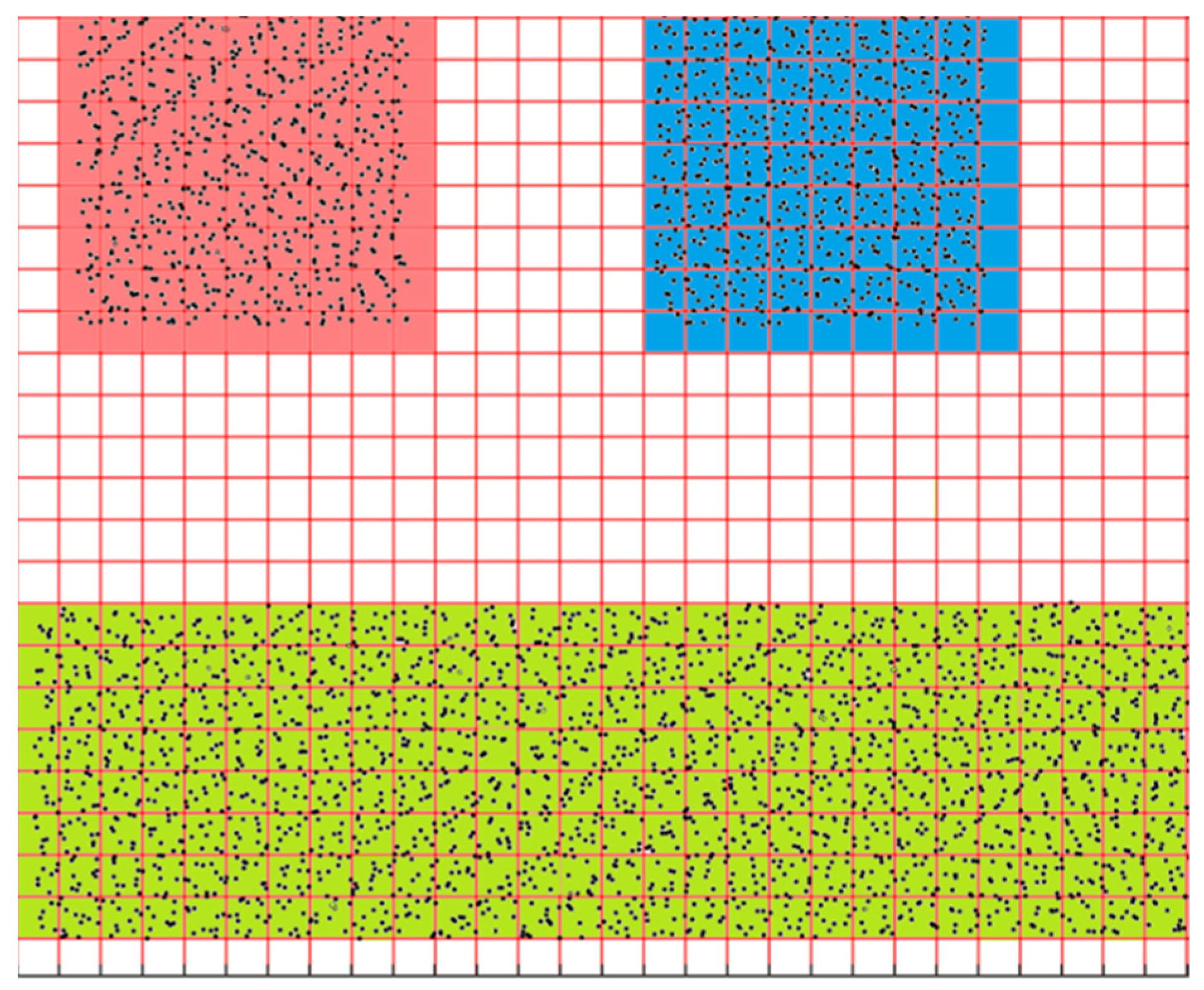
The airborne LiDAR dataset used in this study has been point-wisely classified into different classes (such as ground, vegetation, building, and noise). After the points for building classes are separated from those of other classes, they include points for all buildings in the covered area. Therefore, clustering is first conducted to extract the points of each building. Cluster methods such as K-means and Gaussian Mixture Distribution Cluster could not be used for this task because these methods require the number of buildings as an input parameter, which is unknown ahead of time in most cases. Theoretically, cluster methods such as Mean-Shift, Agglomerative Clustering, and Density-Based Spatial Clustering of Applications with Noise (DBSCAN) [24] that do not need the number of clusters as an input parameter can be used to solve this problem. However, all these algorithms are based on calculating the distance between the points and are thus time-consuming due to the enormous number of LiDAR points involved. To achieve efficient clustering, the grid based DBSCAN algorithm is adopted. All the points are first divided into the 2-D grid on the x-y plane, then the DBSCAN clustering is conducted on the non-empty grid cells that contain points. Once all cells are assigned with a cluster id, the points inside the cells are grouped into the same segment if their associated cells share the same cluster id. For example, Figure 2 shows the 2-D view of the point cloud of three buildings. After the points are divided into a grid, the empty grid cells that do not contain points are discarded and all the non-empty grid cells are separated into three clusters by the DBSCAN algorithm (denoted in red, blue, and green). The points contained in these cells are grouped into three segments accordingly, each of which represents an individual building. Since this procedure uses the grid cells as input, whose amount is much less than that of points, its computational efficiency increases significantly compared to the point-based cluster algorithms.

3.2. Initial Building Outline Generation

After the point cloud of each individual building is extracted, the next step is to generate the initial outline. Our approach consists of two parts: (1) extract the outermost points of building, (2) use the outer points as the input of the recursive convex hull algorithm to generate the initial outline.

3.2.1. Extraction of Outermost Points

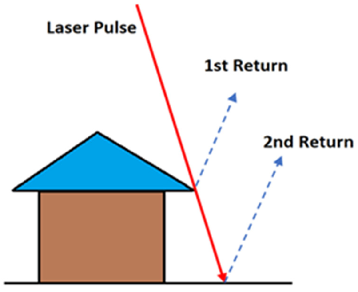
There are two methods introduced here to extract the outermost points. The first one is the multiple-return based method. Multiple-return is a characteristic of linear-mode LiDAR sensors, meaning that one emitted laser pulse could result in multiple received laser pulses. This is because the linear-mode LiDAR emits a laser pulse that has a circular footprint with a certain diameter. When the emitted pulse hit multiple objects with different altitudes, the LiDAR receiver may detect multiple return pulses. As demonstrated in Figure 3, the laser pulse may first hit the eaves of a building before it reaches the ground, generating two returns, one coming from the building eave, and the other from the ground. These two returns are recorded as two 3-D points in the LiDAR dataset, both of which are called “multiple-return points”. Their return number is also stored as an attribute of the point. In this case, the point from the building’s eave has a return number that equals 1 and the other point’s return number equals 2.
The multiple-return property provides a convenient way to extract the points located at the building’s eave. The outermost building points can be easily extracted by selecting the multiple-return points that are classified as building. Figure 4B demonstrates such an example, the multiple-return points extracted are the outermost points of the building.
There are certain cases in which the multiple-return points are not located at the building’s outermost eave. These points may come from chimneys, attics, or other internal objects with their height extruded above the roof. These internal multiple-return points can be removed by checking the point density of their neighborhood region. Since the internal points are surrounded by other points, the point density of their neighborhood is higher than that of the outermost points.
Since the linear-mode LiDAR is the most widely used airborne commercial LiDAR system at present, the multiple-return based method can be used for most datasets. However, it is observed that some buildings’ eave does not have multiple-return points due to the LiDAR scanning direction. Furthermore, some recently invented LiDAR systems such as Geiger mode LiDAR or single-photon LiDAR do not have the capability to collect multiple return points. In these cases, the second method is introduced to handle these situations. The primary procedure of the second method is to check the neighborhood region of each building point. If a point is classified as a building point and it has at least one non-building point falling into the circle centered at the point, it is extracted as the outermost point of a building. The second method can be applied to any pre-classified LiDAR point cloud, with or without multiple returns property, but is computationally less efficient.

3.2.2. Recursive Convex Hull Algorithm

After the outermost points are extracted from a building’s point cloud, they form a set of unordered points instead of a polygon that consists of vertices connected sequentially. Therefore, the next step is to organize the extracted outermost points to form the initial building outline.
As mentioned previously, the traditional convex hull algorithm is not suitable for generating building outlines because many building outlines are concave polygons. To overcome this problem, we adopt an algorithm that recursively makes use of the traditional convex hull algorithm to generate the correct building outline polygon, whether it is concave or convex. A similar idea was used in biology research [25] but has not been used for building footprint generation in existing algorithms.
Taking the building in Figure 4A as an example, its outline is a concave polygon. After applying the convex hull algorithm to the outermost points in Figure 4B only once, the polygon generated (Figure 4C) is apparently not correct since it does not preserve the concave shape at the bottom right corner and some of the outermost points are not on the generated polygon but relatively far from it.
These points that are far from the generated polygon are named “deviated points” and the corresponding line segment that is nearest to the deviated points is defined as a “spurious line”. The deviated points are identified by finding the points that have a distance to their nearest line segment in the polygon greater than a threshold. Then, the convex hull algorithm is applied again only to the deviated points, which generates another small convex polygon, part of which overlaps with the spurious line. When the overlapped part is removed, a new concave polygon (Figure 4D) that correctly preserves the building shape can be formed by combining the remaining lines of polygons. In cases where the building has a very complex outline, it may need to apply multiple iterations of the recursive convex hull algorithm until no “deviated points” can be detected.
By extracting the outermost points and using the recursive convex hull algorithm, the initial building outline can be correctly generated with improved efficiency because the input data (the outermost points) are only a small fraction of the original point cloud. Meanwhile, the time complexity of the recursive convex hull algorithm remains the same as that of the traditional convex hull algorithm (i.e., O ( n × log ( n ) ) ).

3.3. Signal Based Regularization

Following the initial building outline generation, the next procedure is the outline regularization. Unlike most existing approaches that achieve the outline regularization in the 2-D space, the signal-based regularization method developed in this paper tackles this problem from a very different perspective by using the 1-D discrete signal. This algorithm consists of four steps. Firstly, the 2-D initial building outline derived above is transformed into a 1-D discrete signal by calculating the angular deviation at each vertex. Secondly, a denoising procedure is applied to the discrete signal, which results in a noise-reduced signal that aims to represent the holistic geometric structure of the building footprint. Thirdly, unsupervised data clustering is applied to determine the position of the building corner. In the end, the initial building outline is decomposed into multiple parts based on the location of building corners. Each part is mathematically fitted with a straight line, and the final building footprint is reconstructed by assembling these straight lines.

3.3.1. Transforming Initial Building Outline to Discrete Signal

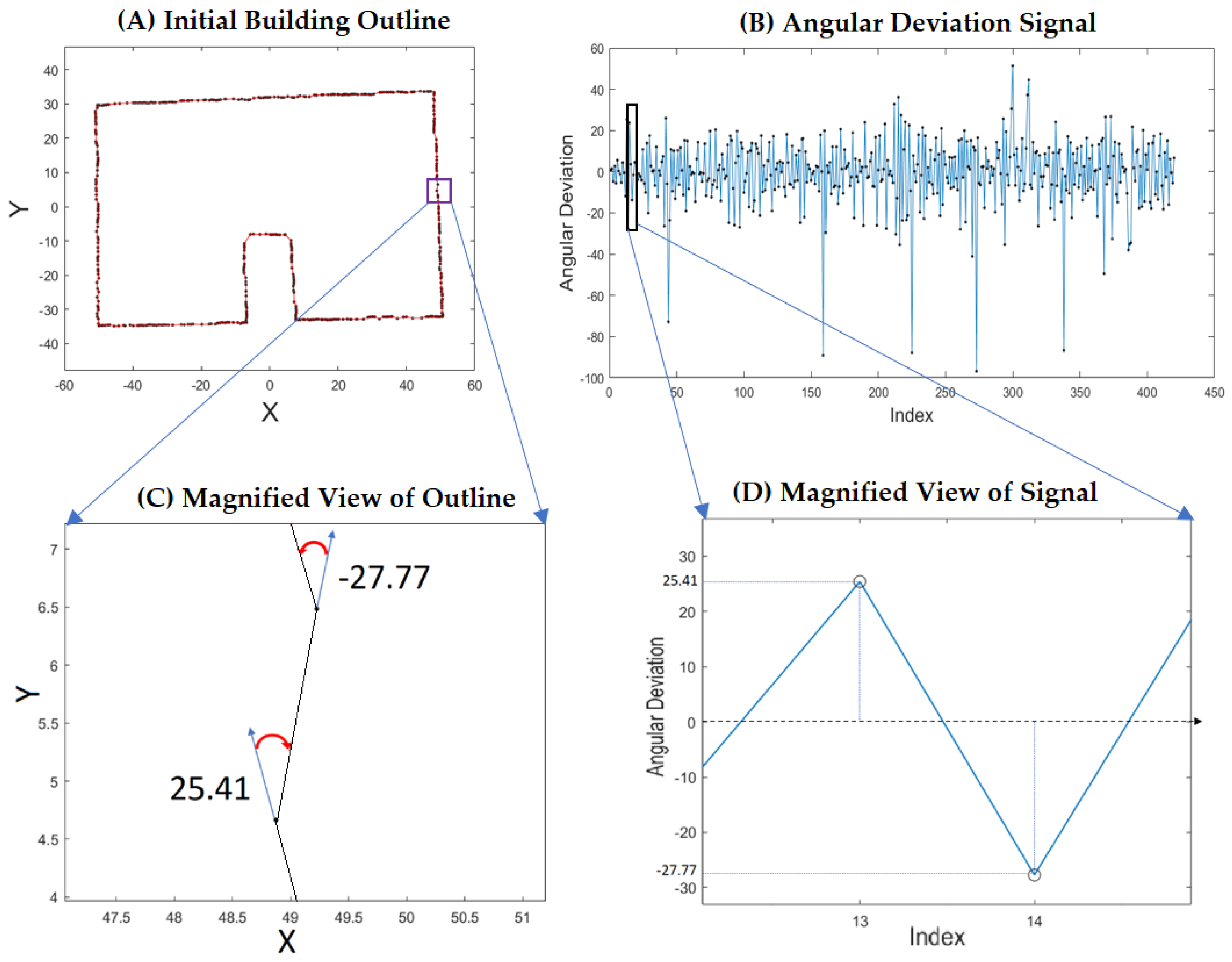
The 1-D discrete signal is essentially a function whose domain is the set of integers. Transforming the initial building outline to a signal is a process of calculating the function value. The detailed procedure is as follows. (1) A random vertex of the initial building outline is selected as the starting point and its index is assigned to be 1. (2) The indices of the other vertices can be determined consecutively based on their order in the initial building outline. (3) Since each vertex connects two adjacent line segments, the angular deviation between the directions of the two line segments is used to formulate the signal. For example, Figure 5A shows an initial building outline and Figure 5C is the magnified view of vertices number 13 and number 14. The angular deviation is 25.41 degrees (clockwise) at vertex 13 and −27.77 degrees (counterclockwise) at vertex 14. Correspondingly, the value of the signal at 13 and 14 are assigned to be 25.41 and −27.77, respectively, as shown in the magnified view of the transformed signal (Figure 5D). Figure 5B is the plot of the entire transformed signal.
The transformed signal is referred to as the angular deviation signal and formally denoted by r [ i ] , where i is an integer that represents the indices of the vertices. Therefore, the signal value at 13 and 14 in Figure 5 are denoted as r [ 13 ] = 25.41 , r [ 14 ] = 27.77 . If an initial building outline consists of n vertices, the values of r [ 1 ] to r [ n ] are equal to the angular deviations at vertices, whereas the value of r [ i ] is equal to 0 when i 0 or i > n .
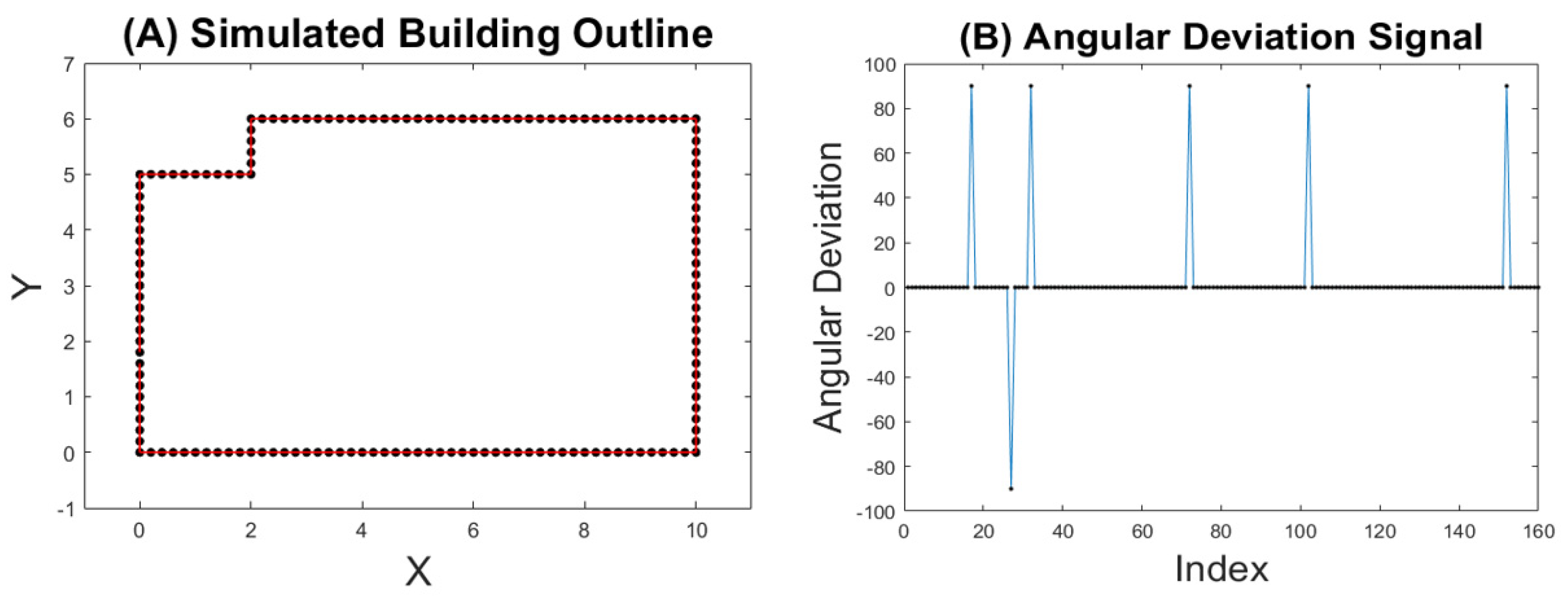
Compared to the 2D polygon, the angular deviation signal provides a simpler way to represent the geometric structure of a building outline. Taking the simulated building outline in Figure 6A as an example, it contains no zig-zag shape and therefore its transformed signal (Figure 6B) has a special pattern, namely 6 spike pulses representing 6 building corners. The indices of the spike pulses are therefore the indices of vertices that represent the building corners.
The angular deviation signal in Figure 5A does not have such a clear pattern to help locate the building corners due to noise caused by the zig-zag shape. In the following section, a denoising procedure is introduced to retrieve such a pattern.

3.3.2. Denoising

Gaussian Smoothing is used as the denoising technique. It is achieved by convoluting the Gaussian smoothing signal with the signal containing noise, formally defined as:
( r g ) [ i ] = m = + r [ i m ] g [ m ] ,
where r [ i ] is the signal containing noise and g [ i ] is the Gaussian smoothing signal that is derived from Gaussian distribution. ( r g ) [ i ] represents the denoising result. According to Equation (1), the signal value of ( r g ) [ i ] is essentially the weighted sum of signal r. The weight is determined by the Gaussian distribution. The parameters of the Gaussian distribution determine the smoothness of the resulting signal.
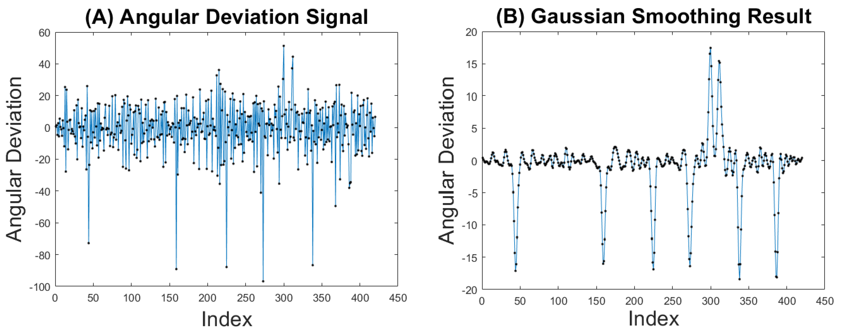
Figure 7 displays the original angular deviation signal and the result after applying Gaussian Smoothing. The noise in the original signal has been significantly reduced and a total of 8 major pulses appear in the resulting signal (Figure 7B). These 8 pulses correspond to the 8 corners of the original building outlined in Figure 5A and therefore are named as “corner pulse”.
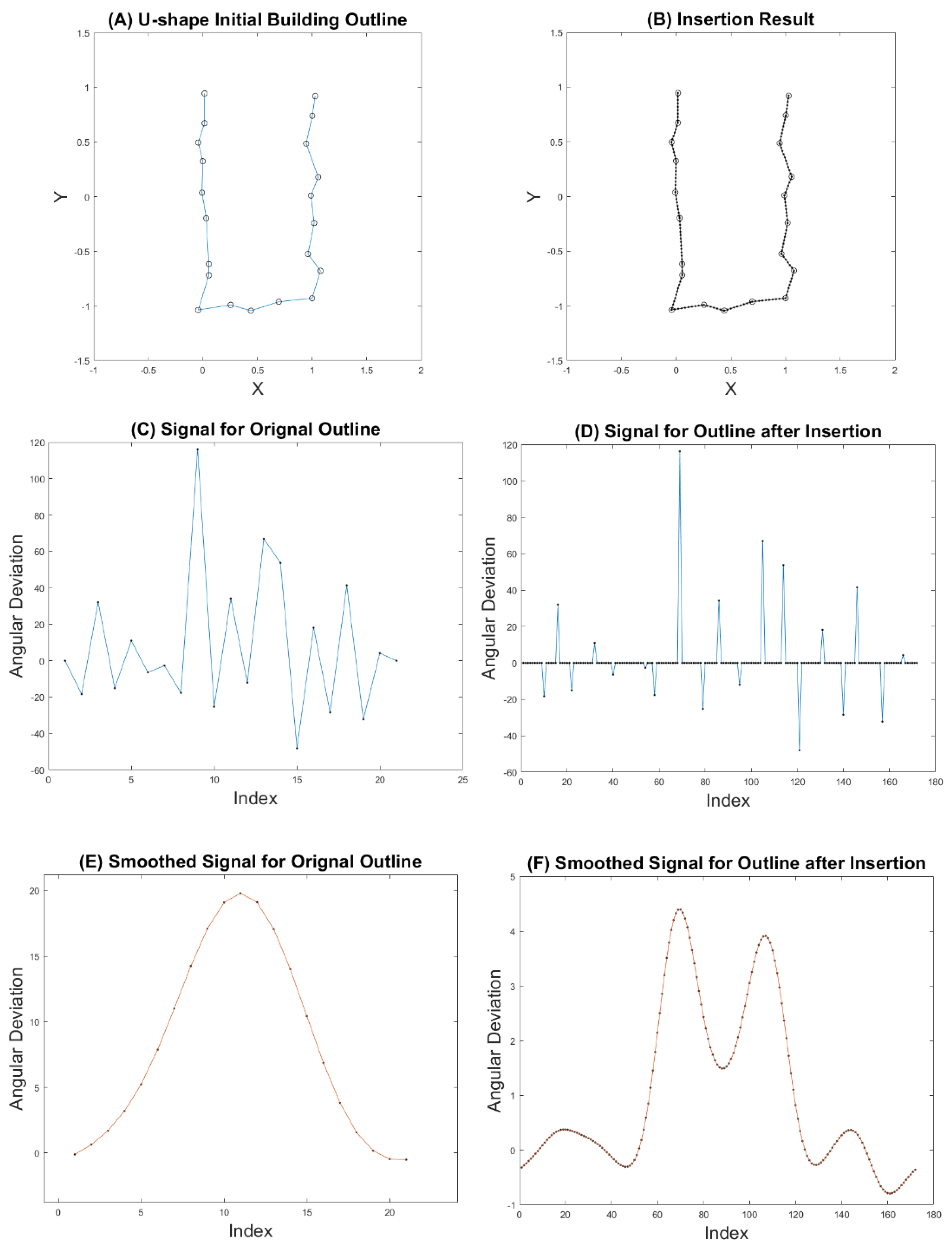
It is found that the Gaussian smoothing not only removes noise but also eliminates the pulses that represent the subtle structure of the building outline. For example, Figure 8A shows an initial building outline with U-shape. It is expected to have two corresponding pulses on the denoised signal. However, after applying Gaussian smoothing, the denoised signal (Figure 8E) shows only one pulse whereas the building outline consists of two corners. This is because these two corners are close to each other, and the distance of their corresponding pulses is shorter than the length of the Gaussian smoothing signal, which makes the two pulses merge into one during the convolution. To correct this problem, an important operation named “insertion” is introduced.
Figure 8B displays the resulting polyline after applying the insertion operation to the initial building outline in Figure 8A. The original LiDAR points are marked with circles and extra vertices (marked with dots) were inserted between two adjacent LiDAR points with a specified distance interval. As the result, the length of the transformed angular deviation signal (Figure 8D) is prolonged compared to the original one (Figure 8C). After Gaussian smoothing, the denoised signal (Figure 8F) now has 2 major pulses, corresponding to the 2 corners in original building outline.
The insertion operation does not alter the geometry structure of the initial building outline but can effectively prevent the Gaussian smoothing from eliminating the subtle structure in the signal. Therefore, the insertion operation is always applied before the Gaussian smoothing.

3.3.3. Identifying Building Corner

The denoising procedure can reduce the noise but still cannot produce the ideal noise-free signal similar to the one displayed in Figure 6B. In Figure 6B, each pulse representing the building corner is a spike that is made of only one non-zero value and therefore has a width equal to one, whereas the corner pulses in Figure 7B and Figure 8F usually consist of multiple non-zero values and have a width larger than one. Additionally, the peak index of the corner pulse in the ideal signal in Figure 6B can precisely indicate the vertex that corresponds to a building corner, whereas the peak index of the corner pulse in Figure 7B and Figure 8F only indicates the vertex close to building corner.
However, the corner pulses in Figure 7B and Figure 8F are still very useful because the approximate building corner locations they provide can be used to decompose the initial building outline into multiple segments. Each segment represents a straight building edge. For example, in Figure 7B, the peaks of the first two corner pulses have indices equal to 48 and 157. Therefore, the vertices whose indices are between 48 and 157 can be used to estimate the parameters of the straight edge connecting these two adjacent corners. In this way, the initial building outline can be disassembled into multiple segments and a final regularized building footprint can be assembled using these straight lines segments.
Based on the description above, identifying the corner pulses from the denoised signal is an important part of the signal-based regularization workflow. In Figure 7B, the identification of the corner pulses can rely on visual interpretation because the amplitude of these 8 pulses is clearly larger than the small-scale fluctuation. However, for cases where the signal is still severely affected by the noise even after Gaussian smoothing, using the amplitude of the pulse as the only criterion to find the corner pulse may not be reliable. Therefore, a clustering-based method is introduced to identify the corner pulses.
The first step of the clustering-based method is to obtain the absolute value of the denoised signal, as shown in Figure 9D. By doing this, the resulting signal can be viewed as a series of pulses with a positive amplitude. The endpoints of each pulse are determined by the indices with local minimum signal value. Each pulse of signal usually has a width larger than 1 and therefore corresponds to multiple vertices in the initial building outline. Taking Figure 9D as an example, the denoised angular deviation signal from 306 to 323 consists of two adjacent pulses. One pulse is from 306 to 318 and the other one is from 318 to 323. Each of these pulses corresponds to a portion of the initial building outline, as displayed in Figure 9B. Based on the plot of the portion, it can be observed that only the first pulse corresponds to a building corner, i.e., it is a corner pulse, and the second pulse is not.
In order to automatically identify the corner pulses, two features are computed for each pulse and its corresponding portion in the initial building outline, namely the angular accumulation and the nonlinear indicator. The angular accumulation of a pulse is calculated by summing all the signal values within the range of this pulse. For example, the angular accumulation of the left pulse in Figure 9D equals the sum of all the signal values between 306 and 318, which equals 178.79. The second feature, the nonlinear indicator, is calculated using the procedure described as follows. (1) Applying the principal component analysis (PCA) to the vertices corresponding to the pulse using their x and y coordinates as input variables, i.e., the coordinates of vertices in the rectangle in Figure 9B. PCA can generate 2 eigenvalues, λ 1 and λ 2 , with λ 1 > λ 2 . (2) λ 2 / ( λ 1 + λ 2 ) is used as the nonlinear indicator because it represents the percentage of the variance of the second component, which is also closely related to the linearity of input data samples (vertices). If all the vertices approximately form a straight line, λ 2 / ( λ 1 + λ 2 ) would be very close to 0. If not, it would be larger. For a corner pulse (such as the left pulse in Figure 9D), its angular accumulation is likely to be relatively large because the angular deviation at the corner is relatively large (close to 90 degrees in this case), and its nonlinear indicator is also expected to be large because the corresponding vertices do not form a straight line. On the contrary, if a pulse is not a corner pulse (such as the right pulse in Figure 9D), the angular accumulation tends to be around 0, and its nonlinear indicator should be close to 0.
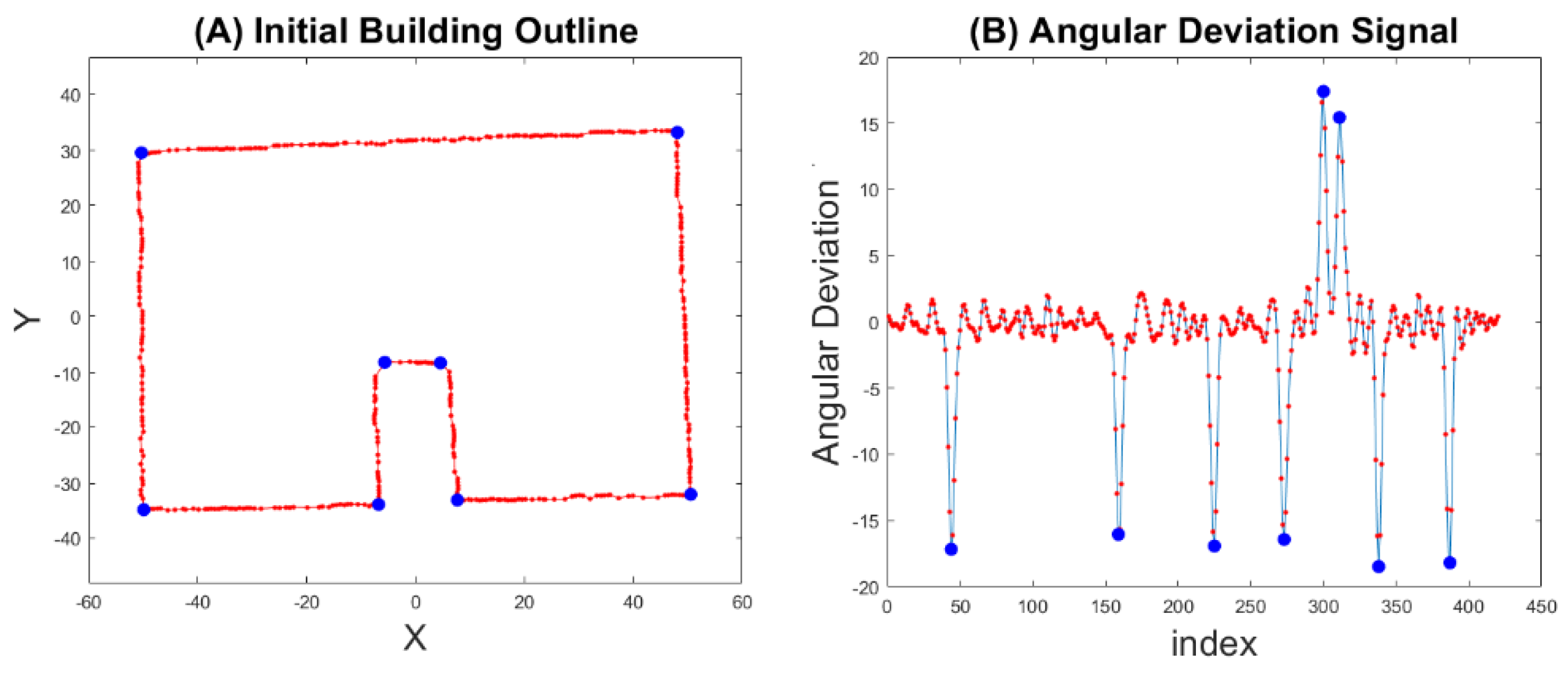
Once the two features are calculated and normalized into the range between 0 and 1, the DBSCAN clustering algorithm is used to separate the corner pulses from the others. Figure 10 displays the feature plot that shows the result of clustering. Every dot corresponds to a pulse with its x coordinate equal to the normalized angular accumulation and y coordinate equal to its normalized nonlinear indicator. As a result, two clusters are formed, with the red dots located near the origin, and the blue dots spread around and away from the origin. As mentioned previously, a pulse with high angular accumulation and a high nonlinear indicator is more likely to be a corner pulse. Therefore, all the dots around the origin point (red dots) are classified as “no corner”, whereas the other dots (blue dots) are classified as “corner”. With the peaks of the pulses that are classified as “corner” being marked on the plot of the denoised signal with blue dots (Figure 11B), and their corresponding vertices also being marked on the initial outline (Figure 11A), all the building corners can be successfully identified.

3.3.4. Reconstructing Building Footprint

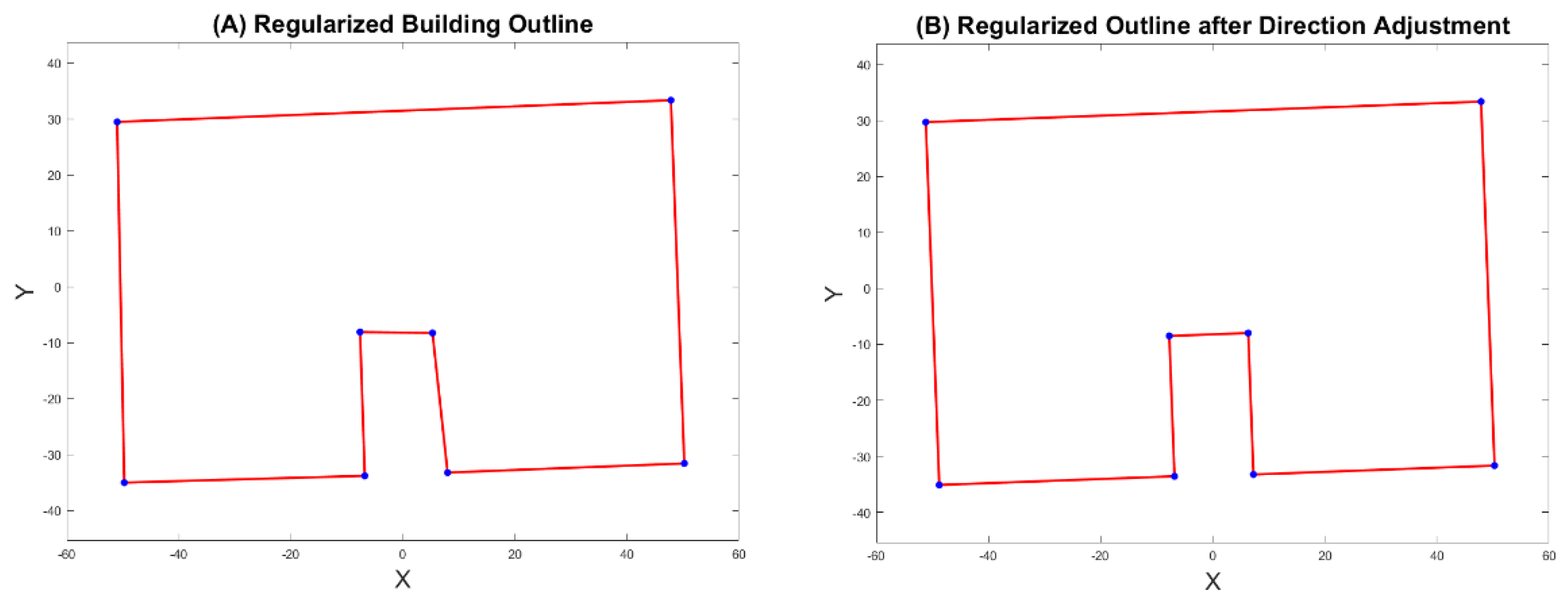
After the corner pulses are identified, the approximate locations of their corresponding building corners can be determined. The last step is to reconstruct a regularized building footprint. As mentioned previously, using the approximate corner locations provided by corner pulses, the initial building outline can be decomposed into multiple parts, each of which consists of several vertices that could form a straight building edge. The coordinates of these vertices are used as the input of the least square approximation to derive the parameters of a straight line. Each two adjacent straight lines have an intersection. Subsequently connecting these intersections results in a regularized building outline without the zig-zag shape, as displayed in Figure 12A.
Although the building outline in Figure 12A has no zig-zags, it is still slightly different from what is expected for this building’s footprint. As a typical building, all the line segments in Figure 12A should be either parallel or perpendicular to each other. Due to the uneven sampling density of the point cloud, the vertices from which the straight line is derived usually have a limited number. Therefore, the direction of the derived straight lines may be slightly away from the actual building edge direction and the perpendicularity between the building edges cannot be preserved. This problem can be corrected by a direction adjustment procedure that is described below. (1) The direction of every line segment in Figure 12A is first calculated and represented by a vector. (2) The angular deviation between every two vectors is calculated. If two vectors are approximately perpendicular or parallel to each other, they are put into the same group. For the vector that is not approximately perpendicular or parallel to any other vectors, it forms a group by itself. In this way, all the vectors are divided into groups. (3) For the groups that contain more than one vector, an average direction is calculated. If the perpendicularity exists between the vectors inside that group. The 90-degree rotation is first performed on those vectors that are approximately perpendicular to most of the other vectors before calculating the average direction. (4) The average direction is used to replace the original direction of the line segment (or rotate 90 degrees if needed), then parallel and perpendicular relationship between the line segments can be recovered, as displayed in Figure 12B. For the vectors that form a single group by themselves, they usually represent an oblique building edge, whose direction will be preserved.

4. Experiment Results

4.1. Test Dataset

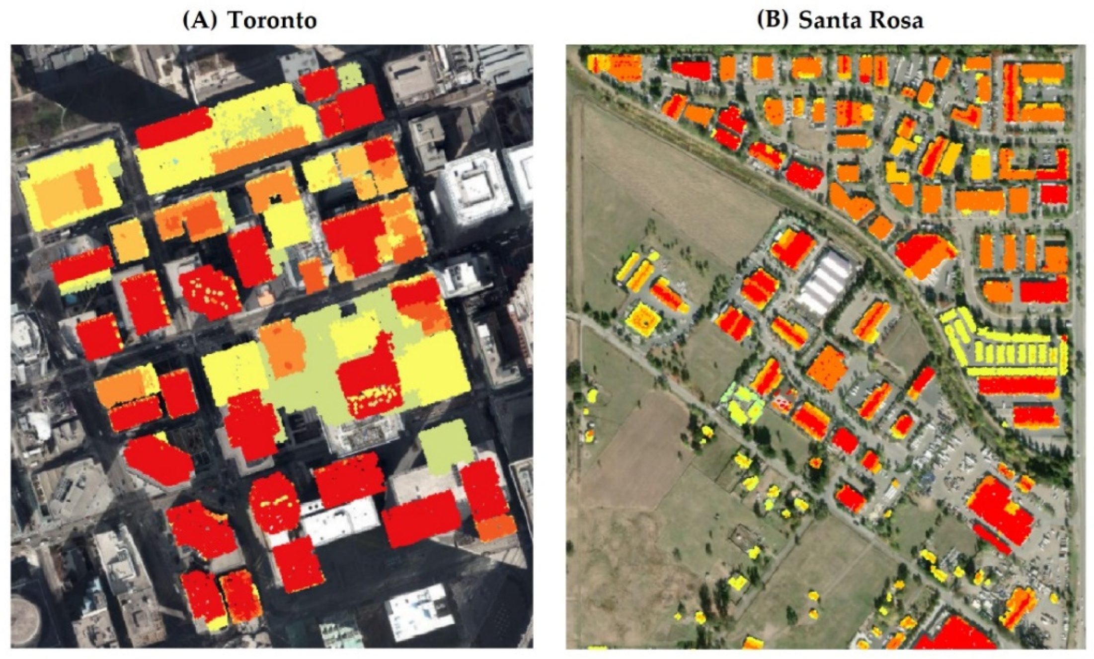
In order to evaluate the performance of the proposed method, the airborne LiDAR dataset collected at Santa Rosa, CA [26] and the ISPRS benchmark dataset for Toronto [27] are used as the test datasets. All the dataset has already been pre-classified. The height-based colorized point cloud of buildings in each dataset on top of airborne imagery is shown in Figure 13A and Figure 13B, respectively.
The reason for choosing these two datasets is that we want to evaluate the performance of the algorithms on datasets with different point densities and different building types. Based on the basic information provided in Table 1, the Santa Rosa dataset contains 115 buildings with a point density of 13.75 points / m 2 , whereas the Toronto dataset contains 34 buildings with a much lower point density that equals 5.95 points / m 2 . Additionally, the buildings in the Santa Rosa dataset have relatively low heights, whereas the buildings in Toronto dataset are mainly high-rise buildings in the city. It is expected that the diversity of test datasets can help to test the robustness of the algorithms.

4.2. Parameter Setting

The grid based DBSCAN clustering, i.e., data pre-processing, is the first part of the workflow. One parameter is needed for grid generation, namely the cell size of the grid. In practice, it is found that the appropriate value of this parameter is closely related to the average spacing (avs) of a point cloud. An acceptable result can be achieved when the cell size is within the range [2 × avs, 5 × avs]. In this study, based on multiple experiments, it is found that the cell size that equals 4 × avs can lead to optimal results. The original DBSCAN clustering has two parameters, epsilon and minPts. Epsilon is the parameter specifying the radius of a neighborhood. minPts specifies the minimum number of neighbor points required to be a core point. Since the grid based DBSCAN is adopted in this study, epsilon is not used. Instead, the eight neighbor grid cells are used to define the neighbor area. Similarly, minCells is used to replace minPts. Its value is set to be 2, meaning that the cell with at least two non-empty neighbor cells is the “core cell”.
After clustering, the recursive convex hull algorithm is applied to the outermost points of each building to generate their initial building outline. The threshold that is used to determine if a polygon has spurious lines is the only parameter in this part. It is noticed that this threshold is also closely related to the average spacing of a point cloud. Based on our experiments, it is found that 3 × avs is the most appropriate value for this threshold.
In terms of the signal-based regularization. There are three parameters in this procedure. The first two parameters are used in the Gaussian Smoothing, which are the standard deviation (sd) and the length (len) of the Gaussian smoothing signal. The value of sd and len directly affect the results of smoothing. A relatively larger value of sd and len can allow Gaussian smoothing to remove more noise and make the resulting signal smoother. However, a too smoothed signal also may cause the subsequent procedure to fail in identifying the corner pulses. The third parameter ε is used by the clustering algorithm DBSCAN. The value of ε affects the accuracy of building corner identification. Its reasonable range is from 0 to 1. However, a too large value of ε would cause DBSCAN fail to detect any building corners and a too-small value can lead to false detection. For different test datasets, the parameter of signal-based regularization may be different due to the different point densities and different building types. Table 2 lists the optimal parameters for two test datasets.

4.3. Result and Evaluation

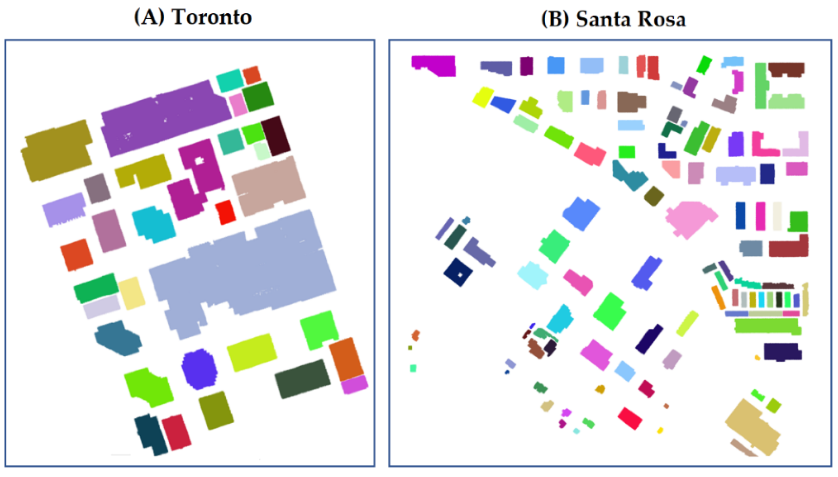
The evaluation is divided into three parts, which correspond to the three parts of the methodology. Firstly, the result of the data pre-processing is evaluated by checking if the point cloud of each individual building can be properly separated from the others. There are two possible clustering errors (1) the point cloud of two nearby buildings is grouped into one cluster; (2) the point cloud of a single building is grouped into multiple clusters. The clustering results are shown in Figure 14, in which the points are colorized with the same color if they share the same cluster id. Based on the qualitative visual examination, the point clouds of all buildings in the test datasets are all correctly separated without any mistakes.
Secondly, the performance of the initial building outline generation algorithm is evaluated by checking if the generated initial building outline correctly preserves the approximate geometric shape of the building boundary. The result is usually very satisfying if the point cloud of each building is correctly extracted, and the parameters are appropriately set. Some researchers introduced quantitative indices to measure the performance of the initial building outline generation [22]. However, given the fact that the indices are usually close to 100%, it is not necessary to quantitatively measure the performance of the initial outline generation. The results of initial building outline generation for Toronto and Santa Rosa datasets are displayed in Figure 15, from which it is observed that the initial building outlines generated correctly maintain the shape of the building boundaries. When the initial outline of a single building is magnified, the zig-zag shape can be clearly noticed.
In order to evaluate the performance of signal-based regularization, the reference building footprint (the ground truth) is generated through onscreen manual digitization using LiDAR point cloud and airborne imagery. The qualitative evaluation is first conducted by visually comparing the regularized building footprint and the reference building footprint. Figure 16 displays the overview of all the building footprints generated by the signal-based regularization algorithm for the Toronto dataset and Santa Rosa dataset. In Figure 17, the magnified view of four representative buildings is presented along with their corresponding initial building outlines, regularized building footprints, reference building footprints, and D-P simplified outline. The first three building footprints are chosen from the Santa Rosa dataset and the last one from Toronto dataset. Overall, the regularized building footprints are almost identical to their ground truth. It is noticed that the second and the third example in Figure 17 as well as the building in the magnified view of Figure 16 do not meet the principal direction assumption. The regularized results for these buildings are quite satisfying, which demonstrates the signal-based regularization achieves its design goal and possesses the ability in generating the correct building footprint that does not have principal directions. Additionally, the second and the third initial building outline in Figure 17 are severely affected by the zig-zag shape. However, the resulting footprints of these buildings successfully recover the shape of building boundary and demonstrates the robustness of the signal-based regularization. The D-P simplified outline is also provided here for comparison. It is obvious that the general simplification not only fails to preserve the sharp feature of building boundary but also fails to eliminate some zig-zag shape.
In addition to the qualitative evaluation, the quantitative evaluation is also performed to precisely measure the difference between regularized building footprint and ground truth. There are no unified quantitative metrics in the existing literature. Different researchers usually use different metrics and criteria to show the accuracy of their results. Some researchers do not even provide any quantitative evaluation. In this study, several most commonly used quantitative metrics are chosen to evaluate the performance of the signal-based regularization algorithm. Additionally, a relatively strict and uncommon quantitative evaluation metric, corner correspondence rate, is also adopted. A detailed description of all the metrics is provided as follows.
  • Intersection over Union (IoU).
I o U = I n t e r s e t e d   a r e a A r e a   o f   u n i o n   o f   b u i l d i n g   f o o t p r i n t s
It evaluates the percentage of the overlapped area between the regularized building footprint and the reference building footprint.
2.
Corner Distance (CD).
C D = 1 n i = 1 n V i R V i s
It measures the average distance between the corners of the reference building footprint and their corresponding corners in the automatically generated building footprint. V i R represents the coordinates of the corners in the reference building footprint. V i s stands for the coordinates of the corners in regularized building footprint. The number n is the total number of corners of the reference building footprint.
3.
Corner Complexity Difference (CCD).
C C D = | n s n r n r |
It measures the difference between regularized building footprint and ground truth in terms of the number of corners. n s equals to the number of corners in the signal-based regularized building footprint. n r equals to the number of corners in reference building footprint.
4.
Corner Correspondence Rate
C C R = n c n c + n m + n f
The corner correspondence rate measures the accuracy of the correct corners by considering both commission and omission errors. By comparing the corners of the regularized building footprint and those of the reference building footprint, a corresponding relation can be established. The corners that have the corresponding relation are regarded as “correct corners”. Their amount is represented by n c . The corners that exist in regularized building footprint but do not have the corresponding relation are regarded as “false corners”, whose amount is denoted by n f . Similarly, the corners in the reference building footprint that do not have the corresponding relation are regarded as “missing corners”, whose amount is n m .
Like much other research, the D-P algorithm is used as the baseline to quantitatively measure the performance improvement of signal-based regularization. The principal direction (P-D) approach [17] is also used in the evaluation.
Table 3 and Table 4 provide the quantitative comparison between all three algorithms using the Toronto dataset and Santa Rosa dataset, respectively. According to the definitions of the metrics, the algorithm with a smaller value for Corner Distance (CD), Corner Complexity Difference (CCD), and larger value for Intersection over Union (IoU), Corner Correspondence Rate (CCR) are superior. Based on Table 3 and Table 4, it is observed that signal-based regularization achieves better performance for all evaluation metrics.
In terms of IoU, it is observed that signal-based regularization has a higher value, although it is not dramatically better than the D-P algorithm and P-D based regularization. Since IoU measures the percentage of the intersected area and the results of all regularization algorithms have a similar shape to the reference building footprint in general, it is expected that the IoU of three algorithms only have minor differences.
CD measures the average distance between the corners of the reference building footprint and their corresponding corners in the automatically generated building footprint. The signal-based regularization also has better and similar results than the other two algorithms, even though the edges of the signal-based regularization result are much closer to those of the reference building footprint compared to the other two. CD only measures the errors in the corner, but not along the edges between the corners. Therefore, a minor difference between all three algorithms was expected.
In terms of the Corner Complexity Difference (CCD) and Corner Correspondence Rate (CCR), signal-based regularization has much better performance than D-P and P-D. Since the D-P algorithm tends to generate some unnecessary vertices, its value for CCD is 89.73% in Santa Rosa, meaning that almost half of the vertices in the D-P simplified building footprint are not necessary, whereas the signal-based regularization has a very low value of 6.82% for this metrics (Table 3). The P-D approach has 216.4% for CCD in Santa Rosa (Table 3), meaning that its result contains excessively more corners than the ground truth. This result is also expected since the Santa Rosa dataset contains many buildings that do not satisfy the principal direction assumption. Toronto dataset contains fewer buildings with edges different from the principal directions, and therefore, the performance of the P-D approach on CCD is reduced to 55.79% (Table 4), much better than that in Santa Rosa.
CCR measures the percentage of the correct corners in all the vertices of the regularized building footprint. D-P only has a value of 52.54% for this metric in Santa Rosa (Table 3) and a value of 66.99% in Toronto (Table 4), meaning that a large portion of the corners in its simplified building footprint is incorrect. Signal-based regularization can achieve a value of 77.82% for the Santa Rosa dataset (Table 3) and a value of 88.21% for the Toronto dataset (Table 4). The P-D approach achieves a value of 36.68% for the metrics in Santa Rosa, meaning that a majority of the detected corners in its regularized building footprint are false corners. Since the Toronto dataset contains fewer edges with directions different from the principal direction, it achieves a value of 81.58% for this metric, much better than D-P but still much lower than the signal-based regularization.

5. Discussion

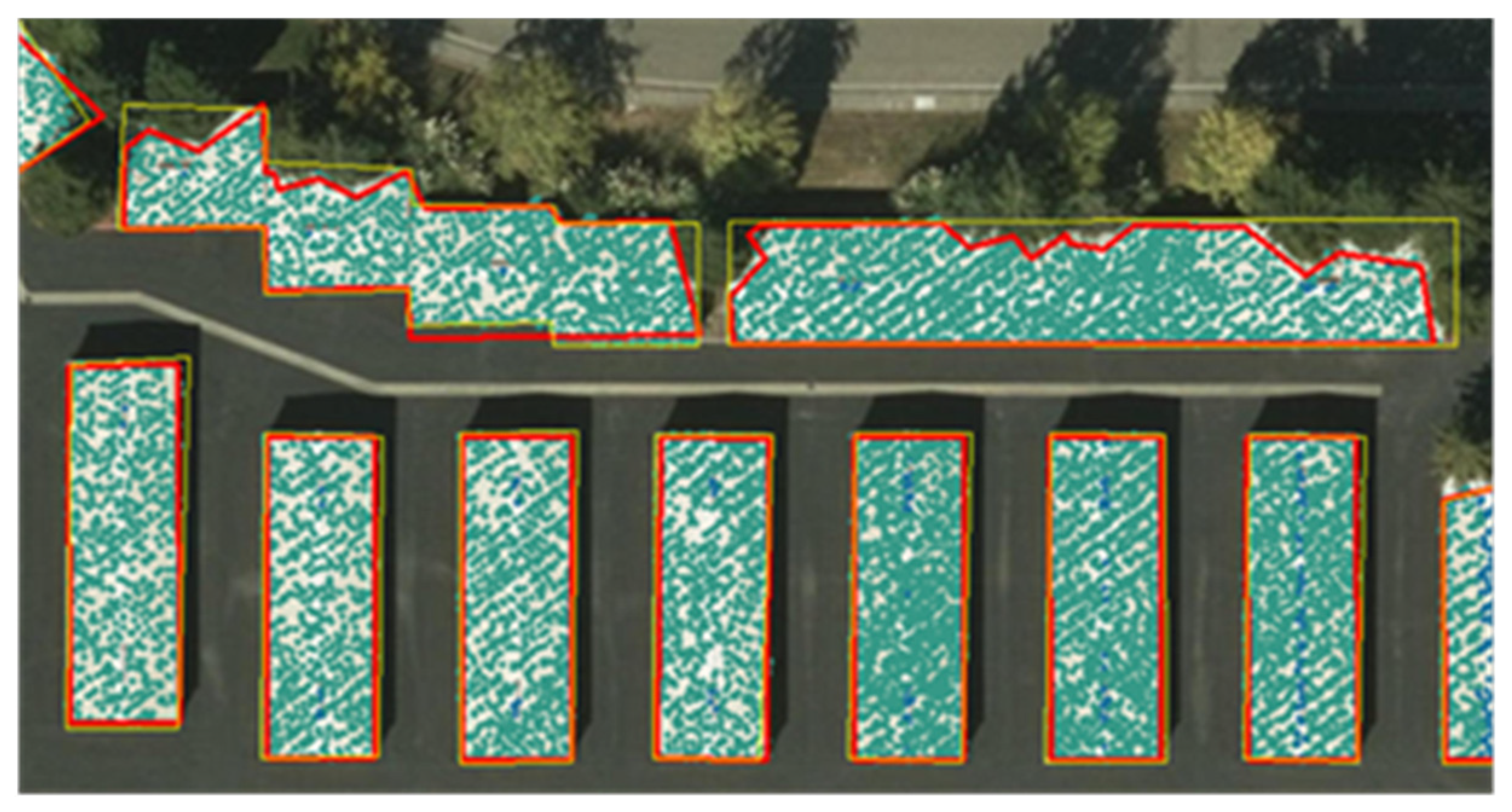
The accuracy of the final building footprint can be affected by many possible factors, such as point density, sensor error, classification error, vegetation occlusion, quality of initial building outline, and robustness of the regularization algorithm. After analyzing all the buildings whose quantitative evaluation results are below the average level, it is found that the vegetation occlusion is the main reason that affects the performance of regularization in the Santa Rosa dataset. Figure 18 displays such an example. The LiDAR points are displayed with overlapped airborne imagery. The yellow polygons are the manually digitized reference building footprints, and the red polygons are the signal-based regularized building footprints. It is clear that two buildings are occluded by the nearby vegetation, which leads to incomplete LiDAR points collected for the buildings. In such cases, it is almost impossible to recover the actual building geometric shape from the point cloud. The buildings in the Santa Rosa dataset have relatively lower heights and therefore are prone to be occluded by nearby vegetation. On the contrary, most buildings in Toronto dataset are high-rising structures and therefore less affected by vegetation occlusion. As observed in Table 3 and Table 4, the signal-based regularization achieved much better performance using the Toronto dataset even though the point density of the Toronto dataset is much lower than the Santa Rosa dataset.
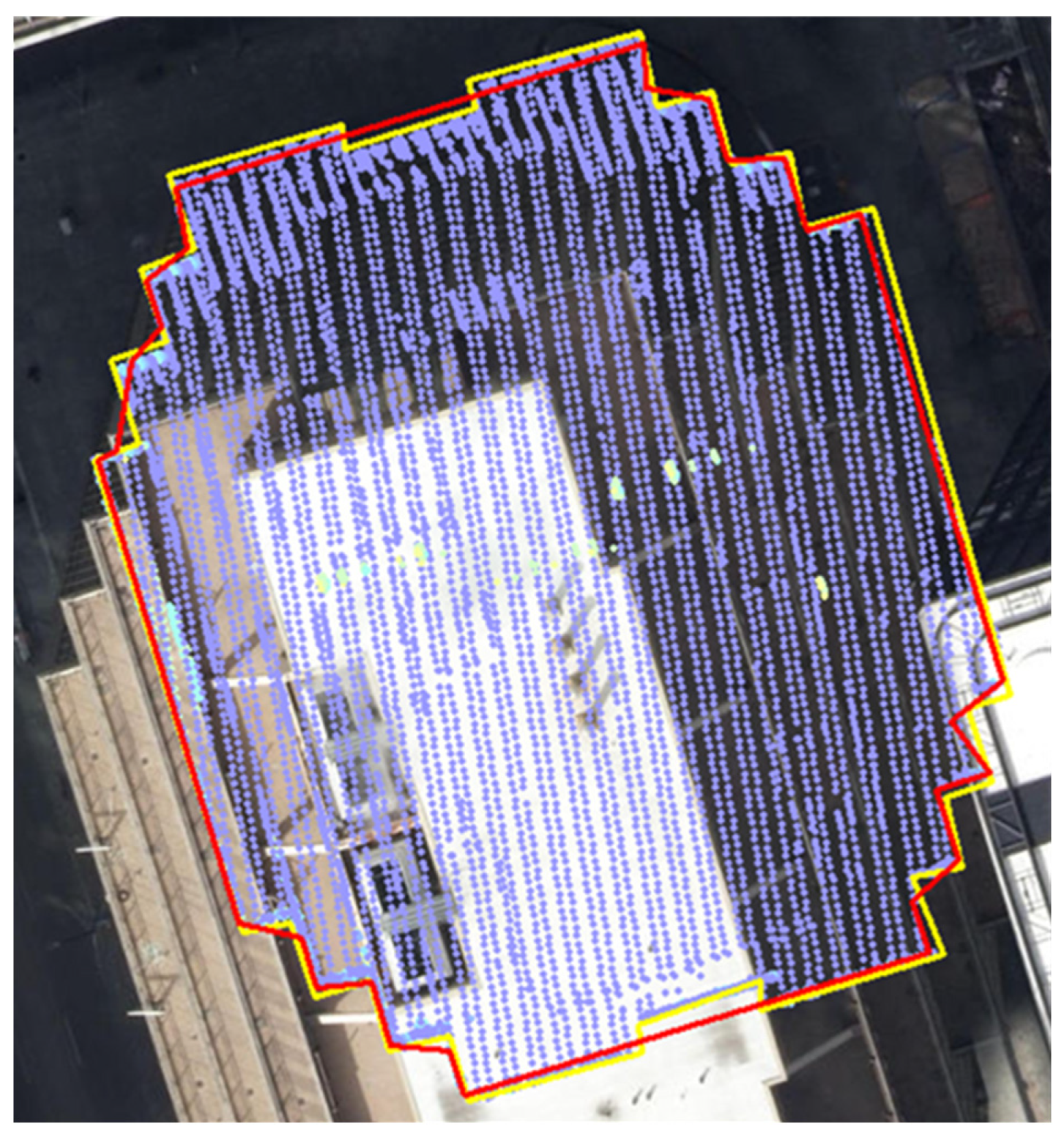
Other than the vegetation occlusion, the uneven point density is found to be the second important factor that influences the performance of the algorithm. Figure 19 shows a building footprint in Toronto dataset that has a less satisfying result. The point cloud is displayed with overlapped airborne imagery. The yellow polygon is the reference building footprint, and the red polygon represents the regularized building footprint. It is obvious that a particular scanning pattern caused by the linear LiDAR system exists in the point cloud. As pointed out by other researchers [16,19], this scanning pattern usually leads to an uneven point density and causes the regularized building footprint to miss some subtle geometric shape even though the overall point density is not low. Therefore, it is anticipated that the algorithms introduced in this research would achieve better results if the data collection can avoid the uneven point density problem.

6. Conclusions

In this paper, an automatic workflow of generating building footprints given a pre-classified LiDAR point cloud is introduced. The workflow consists of three parts. (1) Grid-based DBSCAN clustering is conducted on the pre-classified point cloud to extract the point cloud of each individual building. (2) The outermost points of a single building are extracted, and the recursive convex hull algorithm is used to delineate the initial building outline. (3) The zig-zag shape in the 2-D initial building outline is removed by the signal-based regularization algorithm to generate the acceptable building footprint.
Our main contribution is the algorithms used in the last two parts, namely the recursive hull and signal-based regularization. The advantage of the recursive convex hull algorithm is that only the outermost points are used to generate the initial building outline. As mentioned above, several effective methods are proposed in the literature for delineating the initial building outline. All of them need the entire point set of a building as input, which can have very high computational expense due to the ever-increasing density of an airborne LiDAR point cloud. The recursive convex hull-based approach, on the other hand, starts by extracting the outermost points of a building using the multiple return attributes of LiDAR points, and then applies the traditional convex hull algorithm recursively on the outermost points to generate a proper initial outline of the building. Given the fact that the outermost points constitute only a very small fraction of the entire point set of a building, and the computational complexity of the recursive hull algorithm is the same as the traditional convex hull algorithm, the recursive convex hull algorithm provides an alternative approach for generating an initial building outline with much greater efficiency.
The signal-based regularization is the most important contribution of this research. Unlike any other existing approaches that regularize the initial building outline in the 2-D plane, it first transforms the 2-D initial building outline into a 1-D signal. By doing this, the zig-zag in the 2-D initial building outline is transformed into the noise in signal and the regularization problem becomes the signal denoising problem. The transformation from 2-D outline to 1-D signal reduces the complexity of data and makes it possible to analyze the geometric structure of a building boundary from a different perspective. The final building footprint can be reconstructed after the positions of building corners are detected on the signal. Since this signal-based approach does not have any assumptions regarding the directions of the building boundary, it has the ability to reconstruct proper footprints for the buildings whose boundary has any number of directions.
The most crucial parts of signal-based regularization are reducing the noise in the 1-D signal and detecting the pulses that represent building corners. The techniques that are used to achieve that are Gaussian smoothing and data clustering. It is observed that the accuracy of the resulting building footprint is also sensitive to the parameter setting of Gaussian smoothing. As we mentioned before, a relatively smaller value for the two parameters of Gaussian smoothing is unable to remove enough noise, and a too-large value may cause the subsequent procedure to fail to identify the pulse that represents building corners. The most appropriate parameters have to be carefully chosen to achieve the best results possible. Therefore, future work includes exploring other signal processing techniques to replace the Gaussian smoothing and data clustering to achieve better robustness in performance. Additionally, one major limitation of signal-based regularization is that it cannot generate a curved building edge. Therefore, future work also includes the regularization of a curved building outline. Furthermore, since generating building footprints is usually the first step in the pipeline of creating a 3-D building model, another future work could be incorporating signal-based regularization in automatic 3-D building modeling.

Author Contributions

Conceptualization, X.L. and F.Q.; methodology, X.L.; software, X.L.; validation, X.L., F.Q., F.S. and Y.T.; formal analysis, X.L. and F.Q.; data curation, X.L.; writing—original draft preparation, X.L.; writing—review and editing, F.Q., F.S. and Y.T.; visualization, X.L.; supervision, F.Q. All authors have read and agreed to the published version of the manuscript.

Funding

This research received no external funding.

Data Availability Statement

All datasets used in this article are publicly available through their respective references.

Acknowledgments

The authors would like to acknowledge NASA Grant NNX13AP69G, the University of Maryland, and the Sonoma Vegetation Mapping and Lidar Program for providing LiDAR dataset through https://opentopography.org/ (accessed on 1 July 2022).

Conflicts of Interest

The authors declare no conflict of interest.

References

  1. Shufelt, J.A.; McKeown, D.M. Fusion of monocular cues to detect man-made structures in aerial imagery. CVGIP Image Underst. 1993, 57, 307–330. [Google Scholar] [CrossRef] [Green Version]
  2. Zhang, K.; Yan, J.; Chen, S.C. Automatic construction of building footprints from airborne LIDAR data. IEEE Trans. Geosci. Remote Sens. 2006, 44, 2523–2533. [Google Scholar] [CrossRef] [Green Version]
  3. Gröger, G.; Kolbe, T.H.; Nagel, C.; Häfele, K.H. OGC City Geography Markup Language (CityGML) Encoding Standard 2.0.0; Open Geospatial Consortium: Arlington, VA, USA, 2012. [Google Scholar]
  4. Biljecki, F.; Ledoux, H.; Stoter, J. An improved LOD specification for 3D building models. Comput. Environ. Urban Syst. 2016, 59, 25–37. [Google Scholar] [CrossRef] [Green Version]
  5. Wang, R.; Peethambaran, J.; Chen, D. Lidar point clouds to 3-D urban models: A review. IEEE J. Sel. Top. Appl. Earth Obs. Remote Sens. 2018, 11, 606–627. [Google Scholar] [CrossRef]
  6. McKeown, D.M., Jr.; McGlone, J.C.; Ford, S.J.; Cochran, S.D.; Shufelt, J.A. Automated Cartographic Feature Attribution Using Panchromatic and Hyperspectral Imagery. In Proceedings of the DARPA Image Understanding Workshop, Monterey, CA, USA, 20–23 November 1998; pp. 517–536. [Google Scholar]
  7. Rüther, H.; Martine, H.M.; Mtalo, E.G. Application of snakes and dynamic programming optimisation technique in modeling of buildings in informal settlement areas. ISPRS J. Photogramm. Remote Sens. 2002, 56, 269–282. [Google Scholar] [CrossRef]
  8. Barber, C.B.; Dobkin, D.P.; Huhdanpaa, H. The quickhull algorithm for convex hulls. ACM Trans. Math. Softw. (TOMS) 1996, 22, 469–483. [Google Scholar] [CrossRef] [Green Version]
  9. Douglas, D.H.; Peucker, T.K. Algorithms for the reduction of the number of points required to represent a digitized line or its caricature. Cartogr. Int. J. Geogr. Inf. Geovisualization 1973, 10, 112–122. [Google Scholar] [CrossRef] [Green Version]
  10. Sampath, A.; Shan, J. Building boundary tracing and regularization from airborne LiDAR point clouds. Photogramm. Eng. Remote Sens. 2007, 73, 805–812. [Google Scholar] [CrossRef] [Green Version]
  11. Jarvis, R.A. Computing the shape hull of points in the plane. In Proceedings of the IEEE Computing Society Conference on Pattern Recognition and Image Processing, Troy, NY, USA, 6–8 June 1977; pp. 231–241. [Google Scholar]
  12. Morgan, M.; Habib, A. Interpolation of lidar data and automatic building extraction. In Proceedings of the ACSM-ASPRS Annual Conference, Washington, DC, USA, 19–26 April 2002; Citeseer: Princeton, NJ, USA, 2002; pp. 432–441. [Google Scholar]
  13. Wang, Z.; Schenk, T. Building extraction and reconstruction from lidar data. Int. Arch. Photogramm. Remote Sens. 2000, 33, 958–964. [Google Scholar]
  14. Zhou, Q.Y.; Neumann, U. Fast and extensible building modeling from airborne LiDAR data. In Proceedings of the 16th ACM SIGSPATIAL International Conference on Advances in Geographic Information Systems, Irvine, CA, USA, 5–7 November 2008; pp. 1–8. [Google Scholar]
  15. Edelsbrunner, H.; Kirkpatrick, D.; Seidel, R. On the shape of a set of points in the plane. IEEE Trans. Inf. Theory 1983, 29, 551–559. [Google Scholar] [CrossRef] [Green Version]
  16. Albers, B.; Kada, M.; Wichmann, A. Automatic extraction and regularization of building outlines from airborne lidar point clouds. Int. Arch. Photogramm. Remote Sens. Spat. Inf. Sci. 2016, XLI-B3, 555–560. [Google Scholar] [CrossRef]
  17. Alharthy, A.; Bethel, J. Heuristic filtering and 3D feature extraction from LIDAR data. Int. Arch. Photogramm. Remote Sens. Spat. Inf. Sci. 2002, 34, 29–34. [Google Scholar]
  18. Widyaningrum, E.; Gorte, B.; Lindenbergh, R. Automatic building outline extraction from ALS point clouds by ordered points aided hough transform. Remote Sens. 2019, 11, 1727. [Google Scholar] [CrossRef] [Green Version]
  19. He, Y.; Zhang, C.; Fraser, C.S. An energy minimization approach to automated extraction of regular building footprints from airborne LiDAR data. ISPRS Ann. Photogramm. Remote Sens. Spat. Inf. Sci. 2014, 2, 65. [Google Scholar] [CrossRef] [Green Version]
  20. Jwa, Y.; Sohn, G.; Tao, V.; Cho, W. An implicit geometric regularization of 3d building shape using airborne lidar data. Int. Arch. Photogramm. Remote Sens. XXXVI 2008, 5, 3. [Google Scholar]
  21. Wang, O.; Lodha, S.K.; Helmbold, D.P. A bayesian approach to building footprint extraction from aerial lidar data. In Proceedings of the Third International Symposium on 3D Data Processing, Visualization, and Transmission (3DPVT’06), Chapel Hill, NC, USA, 14–16 June 2006; pp. 192–199. [Google Scholar] [CrossRef] [Green Version]
  22. Awrangjeb, M. Using point cloud data to identify, trace, and regularize the outlines of buildings. Int. J. Remote Sens. 2016, 37, 551–579. [Google Scholar] [CrossRef] [Green Version]
  23. Xu, J.Z.; Wan, Y.C.; Yao, F. A method of 3d building boundary extraction from airborne lidar points cloud. In Proceedings of the 2010 Symposium on Photonics and Optoelectronics, Chengdu, China, 19–21 June 2010; pp. 1–4. [Google Scholar] [CrossRef]
  24. Ester, M.; Kriegel, H.P.; Sander, J.; Xu, X. A density-based algorithm for discovering clusters in large spatial databases with noise. Inkdd 1996, 96, 226–231. [Google Scholar]
  25. Stout, M.; Bacardit, J.; Hirst, J.D.; Krasnogor, N. Prediction of recursive convex hull class assignments for protein residues. Bioinformatics 2008, 24, 916–923. [Google Scholar] [CrossRef] [PubMed] [Green Version]
  26. Dubayah, R.; Hurtt, G. UMD-NASA Carbon Mapping/Sonoma County Vegetation Mapping and LiDAR Program, Distributed by OpenTopography. 2014. Available online: https://doi.org/10.5069/G9G73BM1 (accessed on 21 October 2018). [CrossRef]
  27. Rottensteiner, F.; Sohn, G.; Jung, J.; Gerke, M.; Baillard, C.; Benitez, S.; Breitkopf, U. The ISPRS benchmark on urban object classification and 3D building reconstruction. ISPRS Ann. Photogramm. Remote Sens. Spat. Inf. Sci. I-3 2012, 1, 293–298. [Google Scholar] [CrossRef]
Figure 1. (A) The point cloud of a building and its derived initial outline. (B) The magnified view of the initial outline.
Remotesensing 14 05892 g001
Figure 2. Examples of the grid-based DBSCAN algorithm.
Remotesensing 14 05892 g002
Figure 3. Examples of multiple returns. An emitted laser pulse causes two returns, corresponding to two different LiDAR points. One is for eaves; the other one is for ground.
Remotesensing 14 05892 g003
Figure 4. Initial building outline generation: (A) LiDAR point cloud of an individual building (2−D view). (B) Extracted outermost points. (C) Convex polygon generated after applying convex hull algorithm only once. (D) The concave polygon generated by removing spurious line after applying the recursive convex hull algorithm on the deviated points.
Remotesensing 14 05892 g004
Figure 5. Transforming the initial building outline to discrete signal. (A) The initial outline of a building; (B) The entire plot of the transformed signal; (C) The magnified view of angular deviations at vertex number 13 and number 14; (D) The magnified view of the signal plot when index equals to 13 and 14.
Remotesensing 14 05892 g005
Figure 6. Simulated building outline and corresponding angular deviation signal. (A) The simulated building outline that contains no zig-zag shape; (B) The corresponding angular deviation signal.
Remotesensing 14 05892 g006
Figure 7. Gaussian Smoothing. (A) Angular Deviation Signal. (B) The denoised signal after applying Gaussian Smoothing.
Remotesensing 14 05892 g007
Figure 8. Example of insertion operation. (A) The U-shape building outline; (B) The outline after applying insertion operation; (C) The angular deviation signal of the original U-shape building outline; (D) The angular deviation signal of the outline after insertion; (E) The smoothed signal of original U-shape outline; (F) The smoothed signal of outline after insertion.
Remotesensing 14 05892 g008
Figure 9. Subdivide the denoised signal and calculate features. (A) The initial building outline; (B) the portion of the initial building outline from vertex number 306 to 327; (C) the denoised signal (absolute value); (D) the magnified view of the denoised signal from 306 to 327.
Remotesensing 14 05892 g009
Figure 10. The result of clustering. The Y-coordinate of each dot is the normalized nonlinear indicator. X-coordinate represents the normalized angular accumulation.
Remotesensing 14 05892 g010
Figure 11. The location of the identified building corner on initial outline and their corresponding position on the plot of the signal. (A) All the 8 corners are marked with blue dots; (B) all the peaks of 8 corner pulses are marked with blue dots.
Remotesensing 14 05892 g011
Figure 12. (A) Regularized building outline without the zig-zag shape. (B) Regularized building footprint with adjusted direction.
Remotesensing 14 05892 g012
Figure 13. The point cloud (colorized by height) of test dataset and overlapped airborne imagery (A) Toronto. (B) Santa Rosa.
Remotesensing 14 05892 g013
Figure 14. Points colorized according to its cluster id. Each cluster represents a building. (A) Toronto; (B) Santa Rosa.
Remotesensing 14 05892 g014
Figure 15. Initial Building Outline and magnified view. (A)Toronto. (B) Santa Rosa.
Remotesensing 14 05892 g015
Figure 16. Regularized Building Footprint and magnified view. (A)Toronto. (B) Santa Rosa.
Remotesensing 14 05892 g016
Figure 17. Comparison of Initial Building Outline, Regularized Building Footprint, Reference Building Footprint and D-P Simplified Outline. The first three examples are in the Santa Rosa dataset. The last example is in Toronto dataset.
Remotesensing 14 05892 g017
Figure 18. Example of Vegetation occlusion in Santa Rosa dataset.
Remotesensing 14 05892 g018
Figure 19. Example in Toronto dataset.
Remotesensing 14 05892 g019
Table 1. Basic information of test dataset.
AreaPoint DensityBuilding Number
Santa Rosa 13.75   points / m 2 115
Toronto 5.95   points / m 2 34
Table 2. Parameter setting of signal-based regularization.
Areasdlenε
Santa Rosa1360.25
Toronto1240.2
Table 3. Quantitative Analyses (Santa Rosa).
AlgorithmSignal-Based MethodDouglas–PeuckerPrincipal-Direction
IoU90.37%90.19%90.29 %
CD1.382 m1.797 m1.531 m
CCD6.82 %89.73%216.40%
CCR77.82%52.54%36.68%
Table 4. Quantitative Analyses (Toronto).
AlgorithmSignal-Based MethodDouglas–PeuckerPrincipal-Direction
IoU96.08%95.24%96.01%
CD0.592 m0.922 m0.823 m
CCD5.49%22.12%55.79%
CCR88.21%66.99%81.58%
Publisher’s Note: MDPI stays neutral with regard to jurisdictional claims in published maps and institutional affiliations.