A Novel Estimation Method of Water Surface Micro-Amplitude Wave Frequency for Cross-Media Communication

Abstract

Cross-media communication underpins many vital applications, especially in underwater resource exploration and the biological population monitoring domains. Water surface micro-amplitude wave (WSAW) frequency detection is the key to cross-media communication, where the WSAW frequency can invert the underwater sound source frequency. However, extracting the WSAW frequency information encounters many challenges in a real environment, such as low precision and symbol synchronization, leading to inaccurately estimating the WSAW frequency. Thus, this paper proposed a WSAW frequency estimation method based on an improved RELAX algorithm, incorporating two improvements. First, adding a nonlinear filter to the RELAX kernel function compensates for the filtered gain and enhances the WSAW frequency precision. Second, the improved RELAX kernel function is combined with the generalized inner product method to obtain the time distribution of the non-stationary signals, which is convenient for decoding. Several simulations and experiments applying our method on a Ka-band frequency modulated continuous wave (FMCW) radar demonstrate that our algorithm attains a better performance than traditional methods, e.g., periodogram and the RELAX algorithm. Using the improved algorithm affords to extract the frequency information of the WSAW signal accurately with a short sampling duration, further improving the performance indicators of the communication system, such as communication rate.

1. Introduction

The ocean parameter (velocity and wave height) inversion based on remote sensing means has a wide range of applications in many fields [1,2]. Among these, cross-water–air interface acoustic and electromagnetic integrated communication (AEIC) technology considers an underwater target sending sound signals, which excite the water surface to vibrate. The aerial platform sends radio frequency signals to detect the vibration, restoring underwater information. In recent years, human exploration activities in the ocean have increased, and therefore AEIC has great applications in maritime communication, including water body detection [3,4,5,6], underwater resource exploration [7,8,9], marine biological population monitoring [10,11,12], and underwater target location [13,14,15].

Currently, cross-water–air communication technology is divided into three categories: 1. Buoy technology [16,17], where acoustic-electro conversion and signal processing are realized by setting buoys to complete information transmission from underwater to water. However, this technology suffers from low concealment and high volume power consumption. 2. Opto-acousto communication technology [18,19,20], where the underwater target sends sound signals to excite the water surface to form the water surface micro-amplitude wave (WSAW). Then, laser interference technology is used to detect the WSAW. 3. Acoustic–electromagnetic communication technology [21], unlike opto-acousto communication technology, uses radar signals instead of laser to measure the WSAW. Compared with the opto-acousto communication technology, it has the features of all-weather, large irradiation area, and minimal requirements regarding the measurement platform’s stability. This paper primarily considers acoustic–electromagnetic cross-media communication technology.

In acoustic–electromagnetic communication technology, the information of underwater sound source is inversed by detecting the WSAW. This is because the vibration frequency of the WSAW is identical to the underwater sound source’s frequency, and cross-media communication can be achieved by frequency estimation [22]. Since the WSAW amplitude is only in the order of micrometers [22,23], an accurate spectrum estimation algorithm has an important influence on the WSAW frequency estimation accuracy. In recent years, some research groups use the traditional periodogram (FFT) method to estimate the WSAW frequency based on their radar prototypes [21,24,25]. For instance, in [21], Tonolini designed the translational acoustic-RF communication (TARF) with a carrier frequency of 60 GHz, which was used to estimate the WSAW frequency. In [24], the radar’s center frequency was set to 0.33 THz and was exploited to detect the WSAW. After unwrapping and filtering, the vibration change form of the WSAW was calculated utilizing the periodogram.

However, the periodogram naturally suffers from smearing and spectrum leakage. The smearing problem does not allow the separation of two similar signals, while the spectrum leakage causes the side lobes of the strong signal to overwhelm the weak signal. Thus, the periodogram typically fails to obtain accurate results of the frequency spectrum estimation of minute vibrations [26,27,28]. The periodogram is typically used in cross-media communication, but the periodogram method will fail in the following cases. First, to increase the communication rate, the shorter the signal frequency duration, the higher the communication rate. Short sampling duration will reduce frequency resolution, leading to inaccurate frequency and increasing the communication bit-error rate. Second, the communication frequency band of the underwater speaker is a narrow band range. In order to use multiple frequencies coding in the narrow band, signals of similar frequencies must be separated as much as possible. Third, when the measured signal contains some signals with strong amplitude, the strong signal’s side lobe overwhelms the weak signal’s main lobe, affecting the accurate WSAW frequency estimation. Finally, the periodogram is not suitable for non-stationary signals, but the WSAW signal we receive is a cyclostationary signal.

For the cross-media acoustic and electromagnetic integrated communication technology, estimating the underwater sound source frequency is mandatory. The RELAX algorithm is a spectral estimation algorithm that effectively solves some problems that the periodogram cannot solve. Li introduced the RELAX algorithm in 1996 for target feature extraction [29]. Specifically, Li applied the RELAX algorithm to detect breathing and heartbeat and successfully estimated and separated their frequency [26]. In principle, the RELAX algorithm is a super-resolution algorithm with a high-frequency resolution that effectively solves the first and second problems in the periodogram. However, since it subtracts the estimated maximum value, the side lobe is not suppressed, and therefore applying the RELAX algorithm to the third problem fails. Finally, the cross-media communication scheme sends at least two different frequencies and encodes them, creating a cyclostationary signal. Therefore, we conclude that RELAX is inappropriate for processing cyclostationary signals.

The above-mentioned spectral estimation algorithm is inappropriate for WSAW signals. Hence, to overcome the above problems, this work develops an improved RELAX algorithm. Specifically, we perform nonlinear filtering on the RELAX kernel function to separate similar frequencies. Furthermore, the non-uniformity detection based on the generalized inner product is utilized to obtain the different frequency signals interval so that non-stationary signals can be processed.

The remainder of this paper is organized as follows. Section 2 introduces the underwater sound source excitation model and the detection principle. Section 3 proposes the spectral estimation method based on an improved RELAX algorithm. Section 5 presents the simulation and experimental results, while Section 5 analyzes and discusses the performance obtained. Finally, Section 6 concludes this paper.

2. Underwater Sound Source Excitation and Detection Principle

2.1. Underwater Sound Source Excitation Model

The underwater speakers cause vibrations on the water surface through excitation, and the vibrations formed on the water surface are the WSAW. Figure 1 illustrates the experimental system diagram of the FMCW radar detecting the WSAW, where a signal generator sends a specific frequency signal to the underwater sound source that radiates sound pressure to the water surface. Due to the characteristic impedance mismatch of the two media, the WSAW will be formed on the water surface, with its frequency consistent with the vibration of the underwater source. We use an FMCW radar to detect the WSAW and analyze the underwater sound source information from the detected signal to realize the underwater information transmission to the water.

In Figure 1, it is assumed that the underwater sound source radiates sound waves in the vertical direction, and the distance from the sound source to the water surface is much greater than the wave number $k=2\pi /{\lambda }_{\mathrm{w}}$. Therefore, the propagation rule of underwater sound source radiation can be approximated by the far-field plane wave. Combined with the water wave theory and the perturbation expansion and solution of the governing equation of water surface wave, a three-dimensional mathematical model of WSAW can be obtained:

$$y=\frac{2p_{\mathrm{i}}}{\omega \rho c_{\mathrm{w}}}{\mathrm{e}}^{-\alpha \sqrt{x^2+z^2}}\cos \left(k\sqrt{x^2+z^2}-\omega t\right)$$

(1)

where $p_{\mathrm{i}}$ denotes the sound pressure level, $\omega =2\pi f_{\mathrm{w}}$ is the angular frequency of the underwater sound source, $f_{\mathrm{w}}$ is the frequency of the underwater sound source, ${\lambda }_{\mathrm{w}}$ is the wavelength of the WSAW, $\rho$ is the density of water, and $c_{\mathrm{w}}$ is the acoustic velocity in water, x and z are the axes of the two-dimensional water surface and $\alpha$ is the attenuation coefficient of the WSAW, which is affected by the viscous force in the water media and is determined by the relationship between the wave energy loss per unit time and unit volume and the wave energy [30]. According to the relationship of energy conservation:

$$\alpha =\frac{4\mu k^2\sqrt{kg+{\sigma }^{\prime }{k}^3/\rho }}{\left(g+3{\sigma }^{\prime }{k}^2/\rho \right)}$$

(2)

where $\mu$ is the viscosity coefficient of the water medium, ${\sigma }^{\prime }=72.75\times {10}^{-3} \mathrm{N}/\mathrm{m}$ is the water surface tension coefficient at 25 °C, and $g=9.8066 \mathrm{m}/{\mathrm{s}}^2$ is the acceleration of gravity.

From Equation (1), the frequency of the underwater sound source is consistent with the frequency of the WSAW, i.e., the underwater transmission information demodulation can be achieved by estimating the WSAW frequency and can be approximated with a sine signal.

2.2. Detection Principle

We choose an FMCW radar to measure the WSAW, as such radars have unique advantages that are not available in other radar types. Those are:

High precision: Since the micro-amplitude changes on the water surface are in the order of micrometers, a terahertz-level bandwidth is required to directly measure the distance changes caused by the WSAW, which is unrealistic for a pulsed radar design requirement. Therefore, by measuring the phase change of the beat signal after mixing and filtering the received and the transmitted signals, we estimate the WSAW’s wave height change. The phase change $\varphi \left(t\right)$ of the beat signal can be expressed as:

$$\varphi \left(t\right)=\frac{4\pi \left(h+y\right)}{{\lambda }_{\mathrm{r}}}$$

(3)

where $h$ is the distance between the radar and the calm water surface, $y$ is the wave height of the WSAW, and ${\lambda }_{\mathrm{r}}$ is the wavelength of the radar signal.

From Equation (3), the shorter the wavelength, e.g., millimeter wave or terahertz frequency band, the greater the phase change caused, which is conducive to achieving high-precision phase estimation. However, a too-short wavelength will impose rapid phase wrapping.

Being robust against interference: The WSAW information is mainly reflected in the phase change of the FMCW radar’s beat signal, which is different from the amplitude-modulated signal and is less affected by noise.

Multi-objective separation: An FMCW radar can identify reflective targets at different distances. Indeed, the radar transmits signals to measure the WSAW and can simply separate the WSAW signals from the other interference signals in the environment through different distance bins, extract specific distance bins separately, and analyze the WSAW parameters.

The FMCW expression in the effective interval $T_{\mathrm{e}}\in \left[-\frac{T}{2},\frac{T}{2}\right]$ is:

$$S_{\mathrm{T}}\left(t\right)=A_0{\mathrm{e}}^{2\pi \left(f_{0}t+\frac{\mu t^2}{2}\right)+{\phi }_0},t\in T_{\mathrm{e}}$$

(4)

where $A_0$ denote the amplitude of the transmitted signal, $f_0$ is the center frequency, $t$ is the fast-time, $\mu =B_{\mathrm{r}}/T_{\mathrm{r}}$ is the chirp rate, $B_{\mathrm{r}}$ is the bandwidth, $T_{\mathrm{r}}$ is the pulse width, and ${\phi }_0$ is the initial phase.

The radar illuminates the water surface, generating WSAW due to the excitation of the underwater sound source. Since the echo delay of the received signal is $\tau \left(t\right)={\left(h+y\right)/c}_{\mathrm{r}}$, ($c_{\mathrm{r}}$ is the light speed), then the received signal can be expressed as:

$$S_{\mathrm{R}}\left(t\right)=K_{\mathrm{r}}{S}_{\mathrm{T}}\left(t-\tau \left(t\right)\right)$$

(5)

where $K_{\mathrm{r}}$ is related to the target’s ability to reflect electromagnetic waves and the signal loss in the propagation process.

The received and the transmitted signals are mixed to obtain the beat signal. Considering the actual situation, the vibration speed of the WSAW is much lower than the speed of light. Therefore, we can obtain mixed signals,

$$S_{\mathrm{b},\mathrm{up}}\left(t\right)=\frac{1}{2}{K}_{\mathrm{r}}{A}_0{}^2{\mathrm{e}}^{j2\pi \left[\left(\frac{2\mu \left(h+y\right)}{c_{\mathrm{r}}}\right)t+\frac{4\pi d_0}{{\lambda }_{\mathrm{r}}}+\frac{4\pi y}{{\lambda }_{\mathrm{r}}}\right]},t\in \left[-\frac{T}{2},\frac{T}{2}\right]$$

(6)

The wave height change $y$ of the WSAW is according to the phase change $\Delta \phi =4\pi y/{\lambda }_{\mathrm{r}}$, and is also directly related to the underwater speaker frequency. Finally, the frequency is obtained through spectral estimation.

3. Proposed Algorithm

One of the cross-media communication cores involves demodulating the underwater sound source frequency from the WSAW. Hence, this section proposes and elaborates on an improved RELAX algorithm to estimate the WSAW spectrum.

3.1. Algorithm Theory

The RELAX algorithm estimates the target signal parameters through a nonlinear least square process, affording robustness. Assuming that the received signal has zero mean Gaussian white noise, the underwater sound source sends $K$ signals of different frequencies. After phase extraction, the phases obtained by demodulation include $K$ signals of different frequencies and random noise.

$$y\left(n\right)={\displaystyle \sum _{k=1}^K{a}_k{\mathrm{e}}^{j2\pi f_{k}n+e\left(n\right)}},n=1,\cdots ,N$$

(7)

where $N$ is the sampling point, $a_k$ is the $k^{\mathrm{th}}$ complex amplitude, and $f_k$ is the $k^{\mathrm{th}}$ frequency. The noise $e\left(n\right)$ is complex Gaussian noise with zero mean and variance of ${\sigma }^2$.

From the nonlinear least squares criterion:

$${\left\{f_k,a_k\right\}}_{k=1}^K=\arg \underset{{\left\{f_k,a_k\right\}}_{k=1}^K}{\min }{\Vert \mathit{y}-{\displaystyle \sum _{k=1}^K{a}_k\mathbf{\omega }\left(f_k\right)}\Vert }^2$$

(8)

where $\mathit{y}={\left[y\left(1\right),y\left(2\right),\cdots ,y\left(N-1\right)\right]}^T$ and $\mathbf{\omega }={\left[1,{\mathrm{e}}^{\left(j2\pi f_k\right)},\cdots ,{\mathrm{e}}^{\left(j2\pi f_k\left(N-1\right)\right)}\right]}^T$.

We estimate the amplitude and frequency of the ${\left(p-1\right)}^{\mathrm{th}}$ WSAW, and the remaining signals, including the $p^{\mathrm{th}}$ WSAW signal, can be expressed as:

$${\mathit{y}}_p=\mathit{y}-{\displaystyle \sum _{k=1}^{p-1}{a}_k\mathbf{\omega }\left(f_k\right)}$$

(9)

By minimizing Equations (8) and (9) simultaneously, we obtain the estimated parameter values of the $p^{\mathrm{th}}$ WSAW signal:

$$a_k={\frac{{\mathbf{\omega }}^H\left(f_k\right)y_k}{N}|}_{f_k={\widehat{f}}_k}$$

(10)

$${\widehat{f}}_k=\arg \underset{f_k}{\min }{\Vert \left[I-\frac{\mathbf{\omega }\left(f_k\right){\mathbf{\omega }}^H\left(f_k\right)}{N}\right]{\mathit{y}}_k\Vert }^2=\arg \underset{f_k}{\min }{\left|{\mathbf{\omega }}^H\left(f_k\right){\mathit{y}}_k\right|}^2$$

(11)

The convergence condition of Equation (11) is that the difference between the ${\left(p-1\right)}^{\mathrm{th}}$ value and the $p^{\mathrm{th}}$ value of Equation (9) is less than a given threshold $\epsilon$.

When the side lobes of the strong signals are higher than the main lobes of the weak signals, the RELAX algorithm results will be wrong, because the result of RELAX subtracts the estimated maximum value of each cycle without suppressing the side lobe signal. For example, the underwater sound source transmits four different frequencies, i.e., 100 Hz, 130 Hz, 180 Hz, and 300 Hz signals, and the RELAX algorithm fails to detect the 300 Hz signals in Figure 2. Since the WSAW is a non-stationary signal, the periodogram and the RELAX algorithm are unaware of the time information, and therefore the underwater sound source information cannot be effectively parsed. To solve these problems, we propose the following two improvements.

First improvement: when the measured signal contains some significant signals, the strong signal side lobe overwhelms the weak main lobe signal, affecting the estimation accuracy of the WSAW characteristic parameters.

Windowing is an effective method to suppress side lobes, which, however, brings two problems simultaneously: main lobe broadening and peak drop. The former affects the estimation accuracy, and the latter affects the gain, leading to a significant error during the next iteration. Adding a window can significantly suppress the side lobes and increase the weak signal parameter estimation accuracy. Let $w\left(n\right)$ be the coefficient of the corresponding window function. Then the normalized amplitude gain is defined as:

$$G=\frac{1}{N}{\displaystyle \sum _{n=0}^{N-1}w\left(n\right)}$$

(12)

where $G$ is the signal compensation gain, $N$ is the number of sampling points, and $n$ is the sampling moment.

Due to the peak drop problem, the amplitude signal estimation is inaccurate when calculating the error function in Equation (9), significantly affecting the subsequent parameter estimation. Thus, the core idea to overcome this concern is to use the gain of the window function to compensate for the attenuation of the signal peak and to modify Equations (10) and (11) to obtain:

$$y_{k,W}=Wy-{\displaystyle \sum _{i=1,i\ne k}^K{\widehat{\alpha }}_{i}W{\omega }^H\left(f_i\right)}$$

(13)

$${\widehat{\alpha }}_{k,W}=\frac{{\omega }^H\left(f_k\right)y_{k,W}}{NG}$$

(14)

$${\widehat{f}}_{k,W}=\underset{f_{k,W}}{\arg \max }\frac{{\left|{\omega }^H\left(f_k\right)y_{k,W}\right|}^2}{NG}$$

(15)

where $W$ is the diagonal matrix of window function coefficients $w\left(n\right),n=0,\cdots ,N-1$.

Second improvement: The above analysis applies to stationary signals, but the received signals are cyclostationary, comprising several stationary signals. Additionally, the signals must be processed hierarchically in advance and divided into different sections according to their strengths to achieve accurate frequency estimation.

The received signals are cyclostationary, and the same frequency signal part is stationary. Therefore, determining the stationary signal interval of each same frequency part is necessary. Given that the data is segmented, we calculate the generalized inner product statistics of each data unit sample and compare them against the background statistical characteristics of the entire data to find the strong and weak signal interval points. This is important as the latter points better affect the interval data division of different regions. The specific algorithm flow is presented below:

First, the number of iterations is set., which decreases as the signal SNR increase. To achieve the best possible performance, this work considers 100 iterations.

Next, the generalized inner product is used to calculate the Mahalanobis distance and classify the interval of the different amplitude signals. The adjacent point difference relies on $y\left(n\right)$, and a new sequence $x$ is obtained that is multi-point stratified with a length of $L$, which in turn is used to obtain the sequence $R$.

Then, the difference of the signal sample sets corresponding to the two frequencies is obtained through the $GIP\left(x_l\right)$ data and after calculating the generalized inner product. After that, the $GIP$ variation coefficient is calculated, and the average value and the standard deviation of the coefficient are combined to estimate the interval.

$$R=\frac{1}{L}{\displaystyle \sum _{l=1}^L{x}_l{x}_l{}^T}$$

(16)

$$GIP\left(x_l\right)=x_l{}^{T}R{x}_l$$

(17)

Finally, after obtaining the interval of the different amplitude signals, the improved one is used to estimate the parameters of the signals in each interval, to obtain the underwater sound source parameters ${\widehat{f}}_k$:

$$\left({\widehat{\alpha }}_k,{\widehat{f}}_k\right)=\arg \underset{\left({\alpha }_k,f_k\right)}{\min }{\left|y_n-{\alpha }_1{\mathrm{e}}^{j2\pi f_{1,k}n}-{\alpha }_2{\mathrm{e}}^{j2\pi f_{2,k}n}\right|}^2$$

(18)

where ${\alpha }_1$ and ${\alpha }_2$ are the WSAW amplitudes, and $f_{1,k}$ and $f_{2.k}$ are the WSAW frequencies.

3.2. Implementation Steps

3.2.1. Hilbert Transform

The analysis presented above is conducted in the complex domain, which considers the demodulator’s wave height changes from the beat signal phase to the real signal. However, this strategy does not allow the improved RELAX algorithm to estimate the parameters, and therefore the complex signals are transformed utilizing the Hilbert transform, affording the WSAW parameter estimation.

It should be noted that the signal is converted from a real signal to a complex signal, and thus, when the improved algorithm is used for spectrum analysis, only the positive-axis spectrum is retained. However, to preserve the energy constantly, the amplitude becomes twice the original value, and the final amplitude estimation result is half the original.

3.2.2. Detection of the Number of WSAW

Before executing the algorithm, it is essential to estimate the WSAW number $K$.

Typical approaches include experience value, FFT, and entropy estimation. The first method heavily relies on subjective human experience and is suitable for scenarios where the number of signals is determined. For example, the focus is only on breathing and heartbeat signals for vital signals. The latter two schemes are suitable for most situations but are inefficient for low SNR signals, especially when the WSAW amplitude detected by radar is in the order of microns and thus can easily be overwhelmed by other interference signals. An example of this strategy was developed by Fuchs [31], who proposed an autocorrelation matrix eigendecomposition method based on chi-square statistics that accurately calculated the number of sine waves under low SNR.

The signals $\mathit{y}=\left[y_1,y_2,\cdots ,y_{N-1}\right]$ of the wave height change are demodulated from the phase of the beat signals. These signals are calculated to obtain the autocorrelation matrix ${\hat{\mathit{R}}}_y$, by performing eigendecomposition on the matrix to obtain the corresponding eigenvalues and eigenvectors and arrange them in descending order. We use the eigenvalues of the ranking number and the covariance matrix ${\hat{\mathbf{\sigma }}}_e^2\left(k\right)$ of the estimated noise to obtain the covariance matrix ${\hat{\mathit{Q}}}_k$ of the signal:

$${\mu }_k=\left(\frac{T-N_e+1}{{\hat{\mathbf{\sigma }}}_e^2\left(k\right)}\right){\hat{\mathit{V}}}_k^T{\hat{\mathit{Q}}}_{{}_k}^{-1}{\hat{\mathit{V}}}_k$$

(19)

where $k$ represents the minimum number of eigenvalues, $T$ is the maximum order of perturbation analysis, $N_{\mathrm{e}}$ is the data length, and $\mathit{V}$ is the corresponding eigenvector, which is compared with the chi-square statistical result of the WSAW number.

In Figure 3, the upper part illustrates the estimation result of the autocorrelation matrix decomposition method using chi-square statistics, and the lower part is the periodogram estimation result. Figure 3a indicates that under high SNR, the estimation results of both methods are five, which is consistent with the simulation results. Figure 3b reveals that under low SNR, the first method’s estimation result is consistent with the simulation, and the periodogram-based result is eight due to because of the noise.

The proposed algorithm first requires a Hilbert transform to convert the real signal to a complex. Then we calculate the compensation gain and the number of WSAW. After that, we use both critical improvements presented in Section 3.1 to calculate the non-stationary signal interval points. Finally, we employ the output of the improvement modules to estimate the WSAW frequency of each interval point. Algorithm 1 introduces the improved algorithm for estimating the frequency of WSAW.

Algorithm 1: Improved RELAX to estimate the WSAW parameter.

INPUT: the demodulated WSAW signals; Hilbert transform; Adding window; Computing the gain from Equation (11); Calculating the number of WSAW by Equation (19); Decomposing non-stationary signals into segmented stationary signals 5. Calculating $x$ by the difference between the adjacent points from the windowed signal; 6. Calculating $R$ from Equation (16) and computer $GIP\left(x_l\right)$ from Equation (17); 7. Calculating ${\alpha }_k$ and $f_k$ from Equation (18); 8. Calculating the average value and standard deviation of $GIP$ to get the interval point; Estimating the parameters of each stationary signal 9. Initializing the parameter ${\alpha }_k$ and $f_k$; 10. Estimating the component to be estimated of ${\hat{\mathit{y}}}_{k,W}$ from Equation (13); 11. Calculating ${\widehat{\alpha }}_k$ and ${\widehat{f}}_k$ from Equations (14) and (15); OUTPUT: interval point; ${\widehat{f}}_k$.

4. Simulation and Experiment

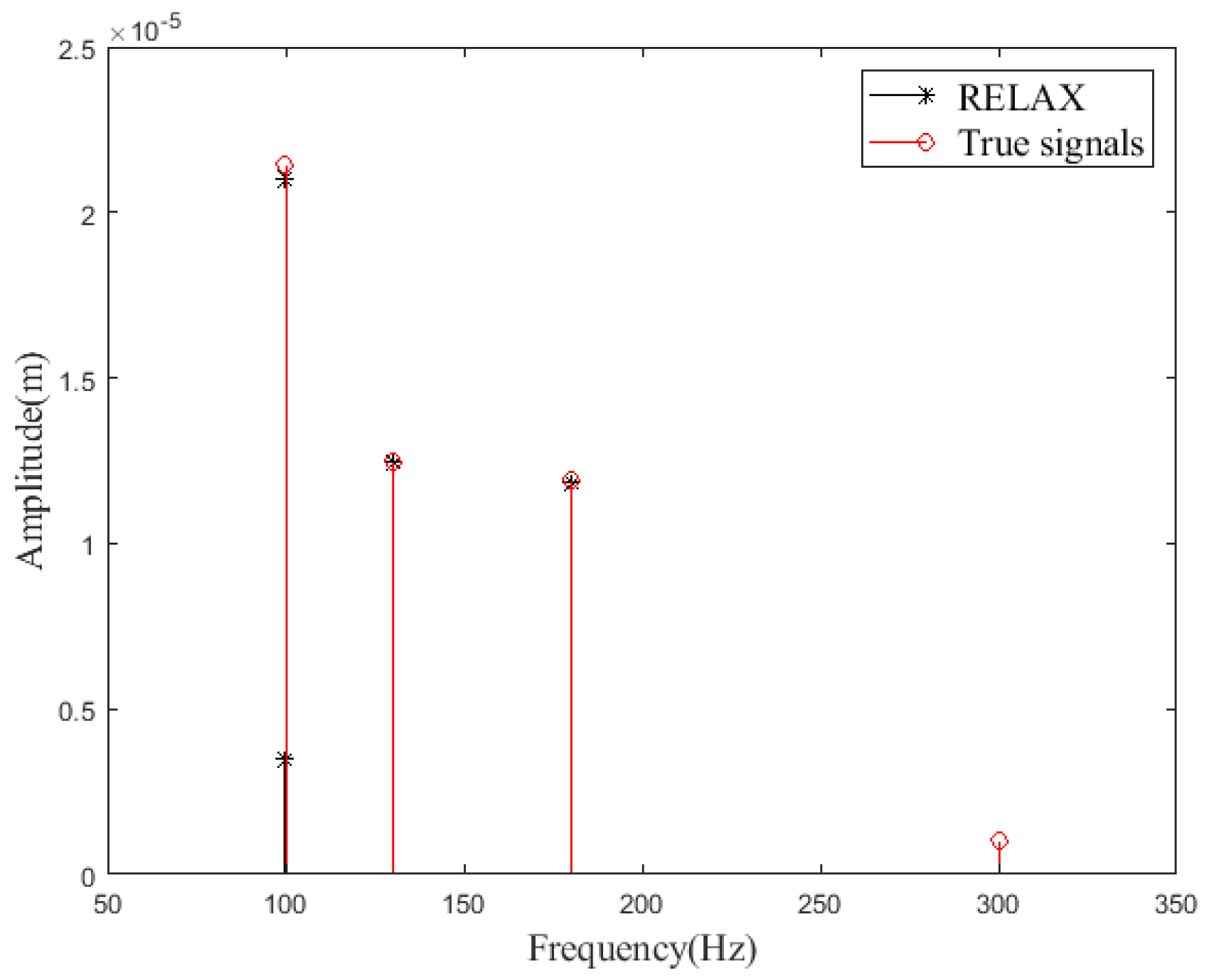
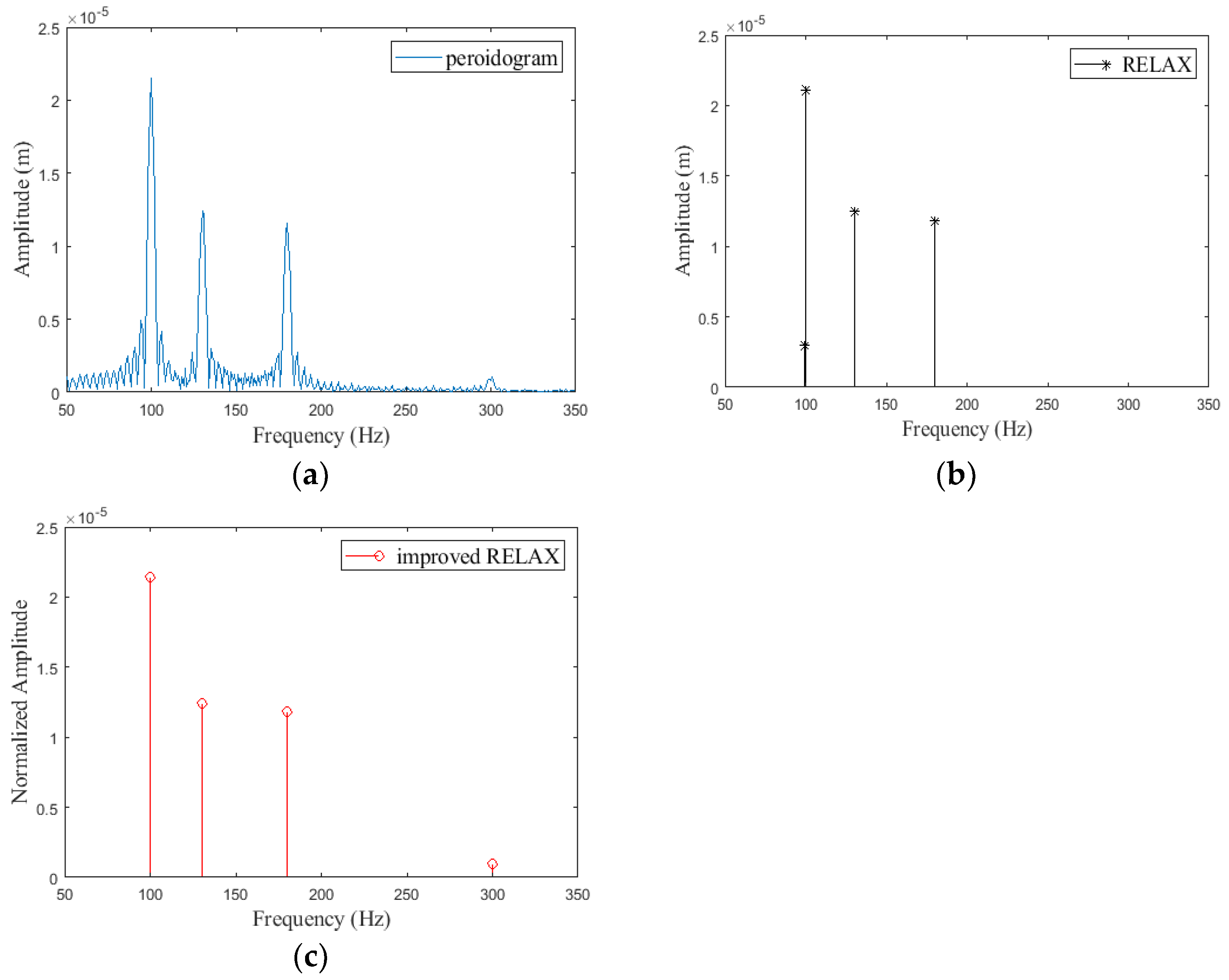
4.1. Simulation Results

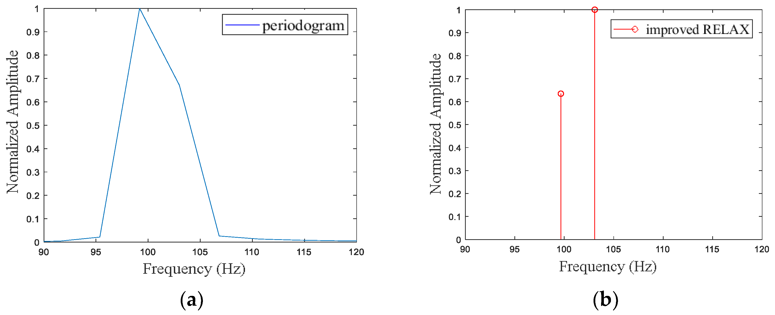
The effectiveness of the improved algorithm is verified on a simulated scenario implemented in MATLAB, involving a micro-amplitude wave model caused by underwater sound sources. The underwater sound source excites signals with two frequencies of 100 Hz and 103 Hz on the water surface, which is also affected by wind.

Table 1. Simulation parameters.

Parameters	Quantity	Value
$R_{\mathrm{radar}}$	distance from the radar to the water surface	1.5 m
$R_{\mathrm{spea}\ker }$	distance from the underwater sound source to the water surface	0.8 m
$L_{\mathrm{p}}$	sound pressure level	110 dB
$f_{\mathrm{w}1}$	transmitting frequency 1 of the underwater source	100 Hz
$f_{\mathrm{w}2}$	transmitting frequency 2 of the underwater source	103 Hz
$B_{\mathrm{r}}$	bandwidth	1.2 GHz
$T_{\mathrm{r}}$	pulse repetition time	8 us
$M$	fast-time sampling number	400
$N$	slow-time sampling number	40,000

reports the FMCW transmitted signal and the simulation parameters.

The echo matrix was obtained from the simulation accumulation of Equation (6). The simulation environment is that the underwater sound source excites 100 Hz and 103 Hz signals to the water surface, superimposed with the sea wave disturbance caused by wind. Since the WSAW amplitude and the sea wave disturbance cannot exceed one range bin, these are represented as a straight line in the echo matrix.

Regarding the method, when a single frequency has fewer sampling data points, the improved algorithm attains a higher estimation accuracy than a periodogram, which requires encoding more frequencies within a certain period, thus increasing the communication system’s transmission rate. Additionally, when the measured signal contains signals with a strong amplitude, the side lobe of this signal overwhelms the main lobe of the weak signal, affecting the accurate estimation of the WSAW frequency. The height of the WSAW is inversely proportional to the frequency of the underwater sound source. If the frequency of the underwater sources is higher, the WSAW reaches the submicron level, making it challenging to detect the WSAW signals. Therefore, the underwater communication frequency band is narrowband. The frequency interval setting for the underwater sound source coding affects the communication performance of the cross-media communication system. However, the improved algorithm can separate the two closer frequencies, thereby improving the underwater acoustic frequency band utilization.

4.1.1. Example One

The first example highlights the importance of the first improvement in a simulation environment. This trial includes three parts, with the first comparing the advantages of the improved algorithm over the periodogram when the amount of the sampled data at a single frequency is relatively small.

The simulated signal frequency is 100 Hz, and the sampling point in Figure 4a,b is 2000 and 20,000, respectively. The improved algorithm and periodogram estimation results are consistent when the sampling points are many. However, when the sampling points are few, the improved algorithm and the periodogram present an estimation error of 1.71% and 8.45% in

Table 2. Estimation error.

Algorithm		Estimation Error
periodogram	91.55 Hz	8.45%
improved RELAX	101.71 Hz	1.71%

, respectively. These results highlight the importance of the suggested algorithm, as even in fewer sampling points, the frequency can still be accurately estimated, encoding more information within a certain period and thus having a faster communication rate.

The second trial considers the frequency intervals. Specifically, the frequency band of underwater communication is narrow, and the improved algorithm supports small frequency intervals for coding, which is convenient for improving the utilization rate of the frequency points in cross-media communication.

The simulation parameters are reported in Table 1. Due to the influence of sea waves, the extracted WSAW signal is filtered to eliminate the influence of low-frequency sea waves. Figure 5a depicts the main lobes of the two peaks as superimposed on the signal of 100 Hz and 103 Hz due to smearing. Therefore, the periodogram cannot effectively distinguish these frequencies. Nevertheless, in Figure 5b, the improved RELAX algorithm distinguishes the two frequencies. The above figure includes 40,000 sampling points, and since the sampling period is eight and the sampling frequency is 125 kHz, the waveform resolution is 3.125 Hz. Therefore, the 100 Hz and 103 Hz signals cannot be separated. However, the improved RELAX algorithm finds the two frequency components and opposes the periodogram, which cannot distinguish the two frequencies due to the small interval. It should be noted that since the improved RELAX algorithm can separate two similar frequencies, more frequency points can be used in a narrow underwater acoustic frequency band.

The third trial considers the actual environment. The water surface is not calm due to external interference. Therefore, the extracted phase contains strong environmental interference. The side lobes of the strong signals cover the weak ones, not detecting the WSAW signal.

Figure 6 infers that when the underwater sound source sends multiple signals continuously, the strong signal’s side lobes will cover the weak signal’s main lobe, but despite that, the improved algorithm can still estimate the weak signal. From Equation (1), it is evident that the amplitude of the WSAW on the water surface is inversely proportional to the frequency of the underwater sound source. Therefore, the side lobe of the low-frequency signal is higher than the main lobe of the high-frequency signal, resulting in decoding errors. In Figure 6, the simulated underwater sound source continuously sends 100 Hz, 130 Hz, 180 Hz, and 300 Hz signals, while Figure 6a illustrates the estimation result of the periodogram. Indeed, the periodogram has large side lobes, with amplitude exceeding the weak signal’s main lobe at 300 Hz, leading to inaccurate estimation results. From Figure 6b, the RELAX algorithm first needs to estimate the strongest signal and then subtract the estimated strongest signal from the original signal. The weak signal will be ignored if the signal has a large side lobe, and therefore the estimated result does not include the 300 Hz signal. In Figure 6c, the improved RELAX algorithm reduces the influence of the side lobes by windowing in advance, compensates for the gain through Equation (12), and the estimation result is consistent with the frequency of the transmitted sound source.

4.1.2. Example Two

Although the WSAW signal is overall non-stationary, it is still a stationary signal during each single-frequency signal. Therefore, it is necessary to identify the interval points between the strong and the weak signals to achieve signal separation. The subsequent trial involves the 100 Hz and 200 Hz signal transmission simulation. In Figure 7, the number of sampling points of the overall signal is 60,000, and the number of sampling points for each single frequency point is 15,000. The intersection of the generalized inner product mean value and the fitted value determines the first interval point at 15,135, the same as the simulation setting frequency conversion point.

4.2. Experiment and Results

The simulation results highlight that the improved method can more accurately estimate the frequency than the periodogram. Thus, this section evaluates the proposed method’s effectiveness on measured data. Specifically, we designed a cross-media communication system, which includes an underwater sound source device that transmits underwater signals, a millimeter wave radar that receives radio frequency signals, and a host for signal processing. The actual measurement experiment aims to verify the advantages of the improved RELAX algorithm for WSAW detection.

The transmitting end of the cross-media communication system is a USW-015 underwater sound source, connected to the audio output port of the host through a power amplifier. The power level of the cross-media communication system is consistent with the standard power acoustic transducer used in the underwater communication process. The signal frequency band of the loudspeaker is set to 100–500 Hz, a typical communication frequency band in underwater communication [32].

The experiment is conducted in a large pool, with Figure 8 illustrating the measurement scene and equipment setup. The transmitting and receiving antennas illuminate the water surface vertically, each placed 0.8 m away from the water surface. The underwater sound source is 0.45 m away from the water surface, and the antenna phase center is aligned with the center of the underwater sound source.

The radar prototype applied in this WSAW detection is designed by the research of the National Key Laboratory of Microwave Imaging Technology, Chinese Academy of Sciences. The radar is a Ka-band FMCW radar, utilizing the two-horn antenna type presented in Figure 8. The radar’s key parameters are presented in

Table 3. Radar parameters.

Parameters	Value
center frequency	34.6 GHz
pulse repetition frequency (PRF)	50 kHz/125 kHz
fast-time sampling points	400/1000
slow-time sampling points	60,000
antenna gain	25 dB

.

The underwater sound source excites the water surface to form a WSAW, which carries the sound source information. Then we transmit a radar signal and receive the echo signal from the FMCW radar. Finally, we extract the phase of the reflected signal to unwrap and filter it to obtain the WSAW vibration signal. The measured signal is sinusoidal, consistent with the underwater sound source model established above.

In this section, we set up two experiments to verify the effectiveness of the improved algorithm. The first experiment considers the first algorithm improvement presented in Section 3. This trial comprises three parts. First, to verify the algorithm’s minimum detectable time, we set the duration of each frequency to 0.001 s, 0.005 s, 0.01 s, 0.05 s, and 0.1 s and compare it with the periodogram to improve the cross-media communication rate. Second, we set the frequency of the underwater sound source to send two signals with a significant difference in frequency simultaneously. Since the amplitude of the WSAW is inversely proportional to the frequency, it is verified that the algorithm can detect the weak signal even when the strong signal covers the weak signal. Third, the minimum detectable frequency range of the proposed algorithm is compared with the periodogram. Since the underwater communication frequency band is narrow, reducing the frequency interval can improve the frequency utilization.

The second set of experiments involves the second algorithm improvement introduced in Section 3. For this case, we estimate the interval points of each frequency.

4.2.1. Example One

The first part aims to verify the minimum sampling duration. The pulse repetition frequency is 125 kHz, and we set five groups of different sampling duration experiments, i.e., 0.001 s, 0.005 s, 0.01 s, 0.05 s, and 0.1 s sampling duration. Figure 9 illustrates the estimation result of the periodogram and the improved RELAX algorithm. Since the frequency of the underwater sound source is 130 Hz, to obtain a complete sine Waveform, the sampling duration must reach 0.0077 s. Neither the first nor the second group can achieve a complete waveform sampling duration, with the estimation results of both methods presenting significant errors. The third set of sampling duration is 0.01 s, the periodogram estimates 125.94 Hz, and the error is 3.15%. The improved RELAX algorithm estimates 129.7 Hz, and the estimated error is 0.23%. Due to the long duration of a single frequency in the fourth and fifth groups, the periodogram and the improved algorithm have estimated the frequency as 129.7 Hz and 130 Hz, respectively, which are the same. The detailed results are reported in

Table 4. Estimation error (transmitted frequency: 130 Hz).

Sampling Duration (s)	Periodogram		Improved RELAX
	Result (Hz)	Error	Result (Hz)	Error
0.005	141.10	8.54%	136.00	4.62%
0.01	125.90	3.15%	129.70	0.23%
0.05	129.70	0.23%	130.00	0.00%
0.1	129.70	0.23%	130.00	0.00%

.

The second part aims to verify the minimum frequency interval when the PRF is 50 kHz. We set the frequency of the underwater sound source to start from 100 Hz, increase by 3 Hz every 0.1 s, and use the periodogram and the improved RELAX algorithm to estimate the detected WSAW signal. Figure 10a illustrates the estimation result of the periodogram, which cannot distinguish two signals with close frequency intervals. Figure 10b depicts the improved RELAX algorithm that successfully separates the two signals of different frequencies. The estimated results are 100.022 Hz and 102.996 Hz, consistent with the actual transmission frequency.

The third experimental part verifies whether the weak signal of the WSAW can be monitored even when covered by the strong signal. In Figure 11a, the periodogram estimation result of the 130 Hz signal has a large side lobe, and its amplitude is larger than the 400 Hz signal. If the frequency is selected from the principle of maximum amplitude, the 400 Hz signal frequency may be missed. In Figure 11b, the RELAX algorithm first estimates the maximum amplitude signal and then subtracts the estimated signal from the original basis, but the side lobe of the 130 Hz signal is greater than the main lobe of the 400 Hz signal. The following estimate is that the frequency of the first side lobe is 144 Hz, which is incorrect. In Figure 11c, the improved RELAX algorithm reduces the side lobes of the signal by windowing the signal in advance. Therefore, the estimated results are 13 Hz and 400 Hz, which are consistent with the signal transmitted by the underwater sound source.

4.2.2. Example Two

The second set of experiments estimates the interval points for solving non-stationary signals given that the WSAW signals considered are non-stationary signals, and the above algorithm is suitable for stationary signals, the amplitude of the WSAW is inversely proportional to the frequencies of the underwater sounder source. Thus, a different sound source frequency corresponds to a different amplitude. After unwrapping, the phase is a piecewise stationary signal, and thus the interval segmentation of each stationary signal can be solved, i.e., the above-mentioned improved RELAX algorithm can be used to estimate the micro-amplitude frequency. In this example, we employ Equation (8) to solve the interval of strong and weak signals, where, the overall data length is 42,000 sampling points, the number of samples is set to 2000, and the data length of each sample is 21 sampling points. Figure 12a highlights that the number of interval points is 1111, and the interval point in the measured data can be calculated as 23,331, which is consistent with the interval point 23,275 obtained from the actual time–frequency analysis diagram of Figure 12b. Therefore, the interval points of different frequencies can be calculated and the WSAW signals are separated.

5. Discussion

In experiments, the frequencies of the underwater sound source are set to $f_0=100,f_1=200$, and the encoding method is 16QAM, with one symbol carrying 4 bits of information. Since the influence of the underwater channel is not considered, the cross-media communication will transmit 100 symbols within 1 s, and then the corresponding data rate is:

$$R_i=100*4=400 \mathrm{bit}/\mathrm{s}$$

(20)

The communication rate is consistent with the highest rate achieved by TARF. Moreover, we can further increase the communication rate by changing the encoding method.

Therefore, we propose an improved RELAX algorithm of the WSAS for cross-media communication. The results suggest that the improved algorithm can improve the frequency accuracy of the WSAS. The proposed algorithm offers a better estimation performance in case of a short signal frequency sampling time. However, the frequency estimation of the periodogram is related to the length of the sampling duration, and specifically, the shorter the duration of a single frequency point, the more inaccurate the estimation result.

Compared with the existing algorithm, the proposed improved RELAX algorithm has three main characteristics. Specifically, the developed scheme first accurately estimates the frequency when there are fewer single-frequency signals, which is beneficial to use more frequency signals for encoding within a certain period, thereby increasing the rate of the communication system. Second, since nonlinear filtering is used to improve the kernel function, the sidelobes of the strong signal are suppressed, affording an accurate estimation of the weak wave signal. Finally, the underwater communication frequency band is a narrow band range. Thus, the developed algorithm can estimate multiple frequencies with a closer frequency interval to improve the utilization of underwater communication frequency points.

Although these studies reveal essential discoveries, some limitations are also worth noting. Combining these schemes with GIP, and according to the inverse relationship between frequency and amplitude and the segmental stability characteristics, the WSAW signal is decomposed into multiple segmented stationary signals to achieve decoding. However, this strategy will increase further the calculation burden compared to the periodogram [33]. Further improvements may be possible using an optimizing parameter, which is a topic for future studies.

6. Conclusions

Accurately estimating the WSAW frequency is one of the main problems in cross-media communication. To overcome this problem, this paper presents an improved RELAX algorithm for WSAS detection, which modifies the traditional RELAX signal model to improve estimation accuracy and applicability. A critical process of the improved algorithm is to perform nonlinear filtering on the data in advance, compensating the filtered gain, thus reducing the influence of side lobe signals. The other critical process is to combine the GIP with the RELAX algorithm to process the non-stationary signals. Finally, the signals are divided into strength signals based on the micro-amplitude signal characteristics, with different signal intervals obtained to achieve normal decoding. The results demonstrate that the proposed method can accurately estimate the micro-amplitude frequency information even if the number of sampling points reduces or the frequency interval is small. Hence, the developed algorithm can improve the communication system’s performance indicators.

References

1. Lama, G.F.C.; Errico, A.; Pasquino, V.; Mirzaei, S.; Preti, F.; Chirico, G.B. Velocity uncertainty quantification based on Riparian vegetation indices in open channels colonized by Phragmites australis. J. Ecohydraulics 2022, 7, 71–76. [Google Scholar] [CrossRef]
2. Tur, R.; Yontem, S. A comparison of soft computing methods for the prediction of wave height parameters. Knowl.-Based Eng. Sci. 2021, 2, 31–64. [Google Scholar] [CrossRef]
3. Bartholomä, A. Acoustic bottom detection and seabed classification in the German Bight, southern North Sea. Geo-Mar. Lett. 2006, 26, 177–184. [Google Scholar] [CrossRef]
4. Yuan, F.; Huang, Y.; Chen, X.; Cheng, E. A biological sensor system using computer vision for water quality monitoring. IEEE Access 2018, 6, 61535–61546. [Google Scholar] [CrossRef]
5. Dietz, A.J.; Klein, I.; Gessner, U.; Frey, C.M.; Kuenzer, C.; Dech, S. Detection of water bodies from AVHRR data—A TIMELINE thematic processor. Remote Sens. 2017, 9, 57. [Google Scholar] [CrossRef] [Green Version]
6. Khan, M.A.; Sharma, N.; Lama, G.F.; Hasan, M.; Garg, R.; Busico, G.; Alharbi, R. Three-dimensional hole size (3DHS) approach for water flow turbulence analysis over emerging sand bars: Flume-scale experiments. Water 2022, 14, 1889. [Google Scholar] [CrossRef]
7. Jarry, J. SAR, NAUTILE, SAGA, ELIT—Four new vehicles for underwater work and exploration: The IFREMER approach. IEEE J. Ocean. Eng. 1986, 3, 413–417. [Google Scholar] [CrossRef]
8. McKnight, S.W.; Dimarzio, C.A.; Li, W.; Hogenboom, D.O.; Sauermann, G.O. Laser-induced acoustic detection of buried objects. In Detection and Remediation Technologies for Mines and Minelike Targets III, Proceedings of the Aerospace/Defense Sensing and Controls, Orlando, FL, USA, 13–17 April 1998; SPIE: Boston, MA, USA, 1998; Volume 3392, pp. 841–847. [Google Scholar]
9. Beverini, N.; Firpi, S.; Guerrini, P.; Maccioni, E.; Maguer, A.; Morganti, M.; Stefani, F.; Trono, C. Fiber laser hydrophone for underwater acoustic surveillance and marine mammals monitoring. In Proceedings of the SPIE—International Conference on Lasers, Applications, and Technologies, Kazan, Russian Federation, 23–27 August 2010; Volume 7994, pp. 285–291. [Google Scholar] [CrossRef]
10. Thomas, G.L.; Hahn, T.; Thorne, R. Combining passive and active underwater acousitics with video and laser optics to assess fish stocks. In Proceedings of the OCEANS 2006, Boston, MA, USA, 18–21 September 2006. [Google Scholar] [CrossRef]
11. Williamson, B.J.; Blondel, P.; Armstrong, E.; Bell, P.S.; Hall, C.; Waggitt, J.J.; Scott, B. A self-contained subsea platform for acoustic monitoring of the environment around marine renewable energy devices-field deployments at wave and tidal energy sites in Orkney, Scotland. IEEE J. Ocean. Eng. 2015, 4, 67–81. [Google Scholar] [CrossRef]
12. Manik, H. Underwater acoustic signal processing for detection and quantification of fish. In Proceedings of the 2011 International Conference on Electrical Engineering and Informatics, Bandung, Indonesia, 17–19 July 2011; pp. 3–5. [Google Scholar] [CrossRef]
13. Ameer, P.M.; Jacob, L. Underwater localization using stochastic proximity embedding and multi-dimensional scaling. Wirel. Netw. 2013, 19, 1679–1690. [Google Scholar] [CrossRef]
14. Liu, C.; Zakharov, Y.V.; Chen, T. Broadband underwater localization of multiple sources using basis pursuit de-noising. IEEE Trans. Signal Process. 2012, 60, 1708–1717. [Google Scholar] [CrossRef]
15. Cho, H.; Gu, J.; Joe, H.; Asada, A.; Yu, S. Acoustic beam profile-based rapid underwater object detection for an imaging sonar. J. Mar. Sci. Tech-Japan. 2015, 20, 180–197. [Google Scholar] [CrossRef]
16. Guerrero, J.A.; Garcia, L.A.; Contreras, J.J.; Buenrostro, R.; Cosio, M. HYRMA: A hybrid routing protocol for marine environments monitoring. IEEE Latin Am. Trans. 2015, 13, 1562–1568. [Google Scholar] [CrossRef]
17. Yoshioka, D.; Sakamoto, H.; Ishihara, Y.; Matsumoto, T.; Timischl, F. Power feeding and data-transmission system using magnetic coupling for an ocean observation mooring buoy. IEEE Trans. Magn. 2007, 43, 2663–2665. [Google Scholar] [CrossRef]
18. Lee, M.; Bourgeois, B.; Hsieh, S.; Martinez, A.; Hickman, G. A laser sensing scheme for detection of underwater acoustic signals. In Proceedings of the 1988 IEEE Southeastcon, Knoxville, TN, USA, 10–13 April 1988; pp. 253–257. [Google Scholar]
19. Antonelli, L.; Blackmon, F. Experimental demonstration of remote, passive acousto-optic sensing. J. Acoust. Soc. Am. 2004, 116, 3393–3403. [Google Scholar] [CrossRef]
20. Blackmon, F.; Antonelli, L. Remote, aerial, trans-layer, linear and non-linear downlink underwater acoustic communication. In Proceedings of the IEEE OCEANS 2006, Boston, MA, USA, 18–21 September 2006. [Google Scholar] [CrossRef]
21. Tonolini, F.; Adib, F. Networking across boundaries: Enabling wireless communication through the water-air interface. In Proceedings of the ACM SIGCOMM 2018—2018 ACM Special Interest Group on Data Communication, Budapest, Hungary, 20–25 August 2018; pp. 117–131. [Google Scholar] [CrossRef]
22. Lurton, X. An Introduction to Underwater Acoustics: Principles and Applications; Springer Science & Business Media: Berlin, Germany, 2002; p. 106. [Google Scholar]
23. Churnside, J.; Bravo, H.; Naugolnykh, K. Effects of underwater sound and surface ripples on scattered laser light. Acoust. Phys. 2008, 54, 204–209. [Google Scholar] [CrossRef]
24. Guo, C.; Deng, B.; Yang, Q.; Wang, H.; Liu, K. Modeling and simulation of water-surface vibration due to acoustic signals for detection with terahertz radar. In Proceedings of the UCMMT 2019—2019 UK-Europe-China Workshop on Millimeter Waves and Terahertz Technologies, London, UK, 20–22 August 2019. [Google Scholar] [CrossRef]
25. Moniara, R. Wireless underwater-to-air communications via water surface modulation and radar detection. In Proceedings of the Radar Sensor Technology XXIV, Anaheim, CA, USA, 26–30 April 2020. [Google Scholar] [CrossRef]
26. Li, C.; Ling, J.; Li, J.; Lin, J. Accurate doppler radar noncontact vital sign detection using the RELAX algorithm. IEEE Trans. Instrum. Meas. 2010, 3, 687–695. [Google Scholar]
27. Li, C.; Lin, J. Optimal carrier frequency of non-contact vital sign detectors. In Proceedings of the 2007 IEEE Radio and Wireless Symposium, Long Beach, CA, USA, 9–11 January 2007; pp. 281–284. [Google Scholar] [CrossRef]
28. Xiong, Y.; Peng, Z.; Xing, G.; Zhang, W.; Meng, G. Accurate and robust displacement measurement for FMCW radar vibration monitoring. IEEE Sens. J. 2018, 18, 1131–1139. [Google Scholar] [CrossRef]
29. Li, J.; Stoica, P. Efficient mixed-spectrum estimation with applications to target feature extraction. IEEE Trans. Signal Process. 1996, 44, 281–295. [Google Scholar] [CrossRef]
30. Zhang, L.; Zhang, X.; Tang, W. Amplitude measurement to weak sinusoidal water surface acoustic wave using laser interferometer. Chin. Opt. Lett. 2015, 13, 091202. [Google Scholar] [CrossRef]
31. Fuchs, J. Estimating the number of sinusoids in additive white noise. IEEE Trans. Acoust. Signal Process. 1988, 36, 1846–1853. [Google Scholar] [CrossRef]
32. Zhou, S.; Wang, Z. OFDM for Underwater Acoustic-Communications; Wiley: New York, NY, USA, 2014; pp. 2–8. [Google Scholar]
33. Liu, Z.; Li, J. Implementation of the RELAX algorithm. IEEE Trans. Aero. Elec. Sys. 1998, 34, 657–664. [Google Scholar] [CrossRef]
Figure 1. Schematic diagram of the experimental system.
Remotesensing 14 05889 g001
Figure 2. The underwater sound source sends 100 Hz, 130 Hz, 180 Hz, and 300 Hz signals, the RELAX fails to estimate the 300 Hz signals.
Remotesensing 14 05889 g002
Figure 3. Estimation of the WSAW number, where the simulated underwater sound source excites five signals of different frequencies. (a) It shows the estimation results of the above algorithm and periodogram under high SNR and (b) low SNR conditions.
Remotesensing 14 05889 g003
Figure 4. The influence of the sampling point cardinality at a single frequency on frequency estimation, involving a signal frequency sampling point of (a) 2000 and (b) 20,000.
Remotesensing 14 05889 g004
Figure 5. Estimation results of (a) periodogram and (b) improved RELAX algorithm.
Remotesensing 14 05889 g005
Figure 6. The underwater sound source sends four different frequency signals. The results of different frequency estimation algorithms based on (a) periodogram that presents large side lobes, (b) RELAX that misses the 300 Hz signal, and (c) improved RELAX, which has estimated results consistent with the frequency of the transmitted sound source.
Remotesensing 14 05889 g006
Figure 7. (a) Generalized inner product value of each sample, and (b) time–frequency analysis result of simulation data.
Remotesensing 14 05889 g007
Figure 8. Cross-media communication platform construction.
Remotesensing 14 05889 g008
Figure 9. The estimated results of the periodogram and the improved algorithm at five different durations, where thebule line and the red line represent the estimated results of periodogram and improved algorithm, respectively.
Remotesensing 14 05889 g009
Figure 10. Verification of the minimum frequency interval (a) periodogram, which cannot distinguish the 100 Hz and 130 Hz signals, and (b) improved RELAX obtaining 100.022 Hz and 102.996 Hz.
Remotesensing 14 05889 g010
Figure 11. Weak WSAW, (a) signal detection based on periodogram, where the amplitude of the 130 Hz signal side lobe is greater than the amplitude of the 400 Hz signal (b) frequency estimation results of RELAX algorithm are 130 Hz and 144 Hz. (c) frequency estimation results of the improved RELAX algorithm 130 Hz and 400 Hz.
Remotesensing 14 05889 g011
Figure 12. (a) Sample generalized inner product value; (b) time–frequency analysis result.
Remotesensing 14 05889 g012