

A Novel Echo Separation Scheme for Space-Time Waveform-Encoding SAR Based on the Second-Order Cone Programming (SOCP) Beamformer

 ,
,  ,
,
Abstract
1. Introduction
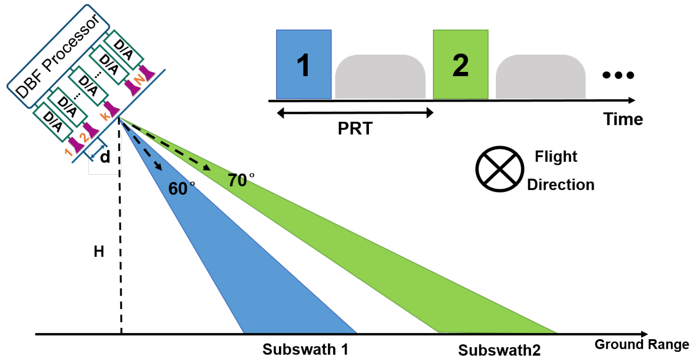
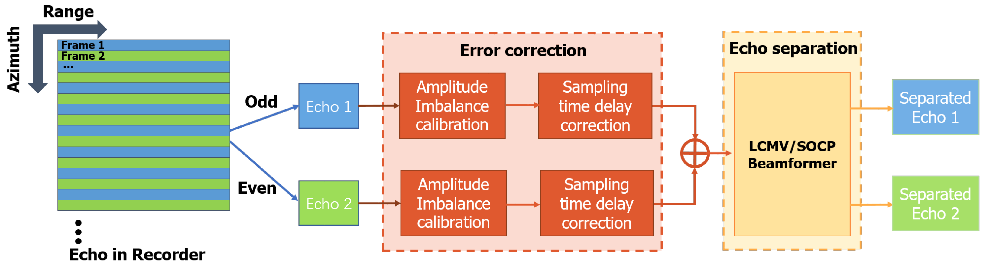
2. Materials and Methods
2.1. Signal Energy Differences
2.2. Deficiencies of the LCMV Beamformer
2.2.1. LCMV Beamformer
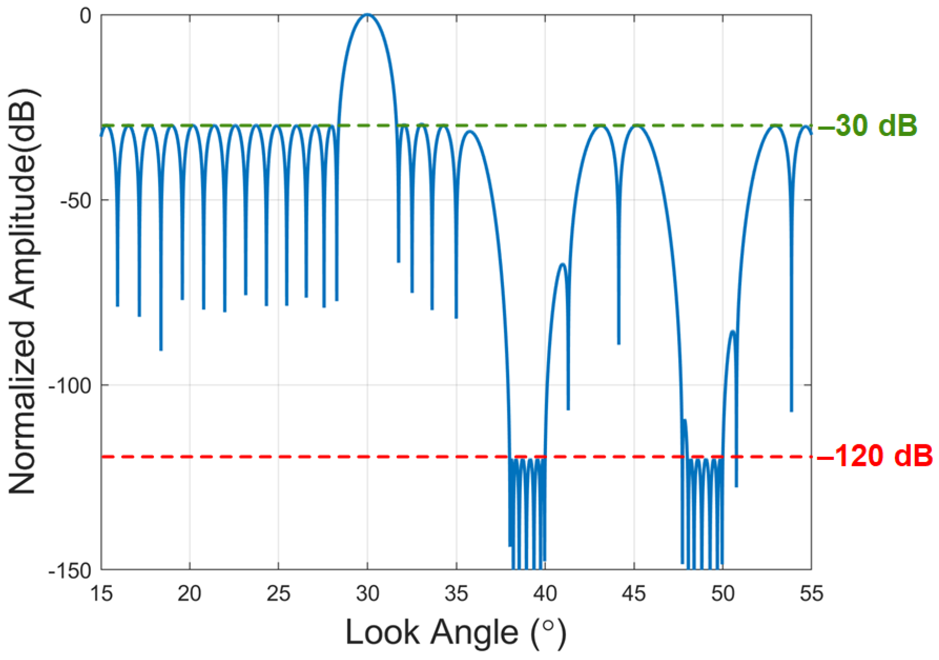
2.2.2. Restricted Notch Depth
2.2.3. Restricted Notch Width
2.3. Proposed SOCP Beamformer
2.3.1. SOCP Theory
2.3.2. Design of the Beamformer Based on SOCP Theory
3. Results
3.1. Simulation Results
3.2. Experimental Results
3.2.1. Effect of Signal Energy Differences
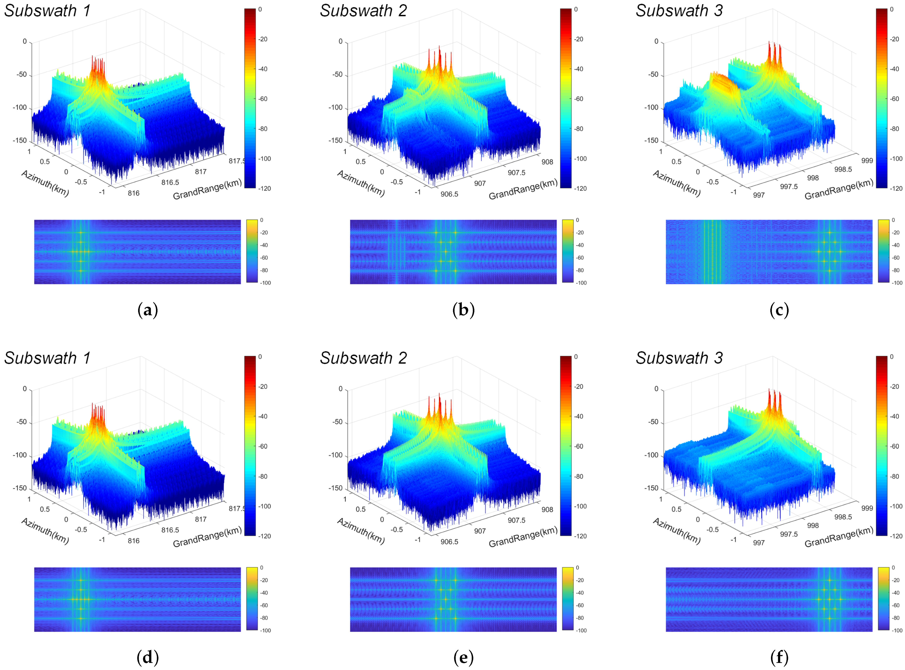
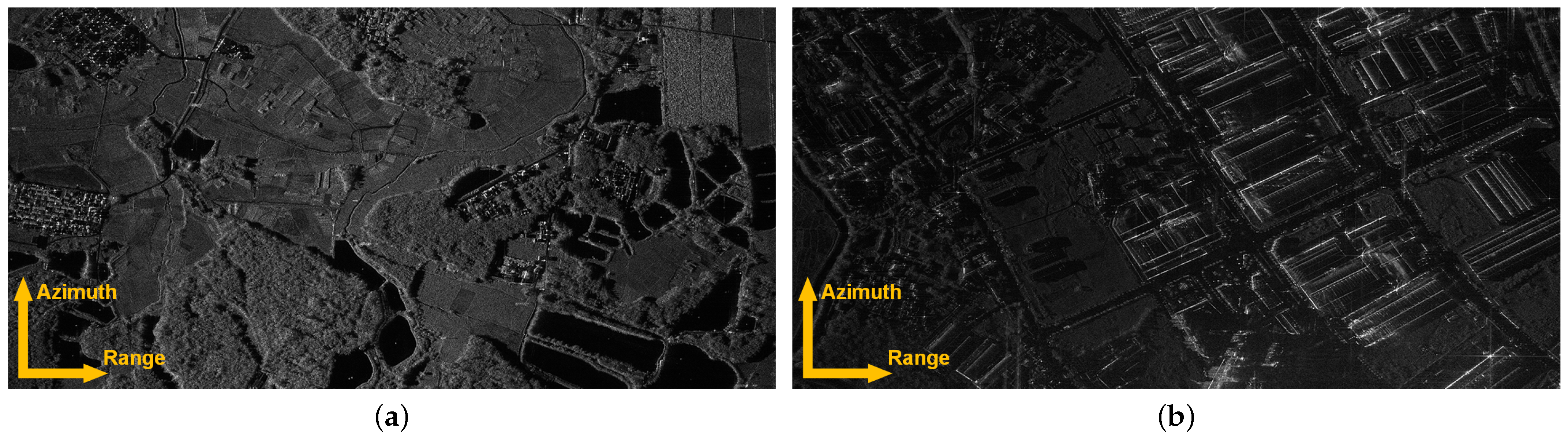
3.2.2. Comparison of Echo Separation Results
4. Discussion
5. Conclusions
Author Contributions
Funding
Data Availability Statement
Conflicts of Interest
References
- Wollstadt, S.; Lopez-Dekker, P.; De Zan, F.; Younis, M. Design principles and considerations for spaceborne ATI SAR-based observations of ocean surface velocity vectors. IEEE Trans. Geosci. Remote Sens. 2017, 55, 4500–4519. [Google Scholar] [CrossRef]
- De Almeida, F.Q.; Younis, M.; Krieger, G.; Moreira, A. Multichannel staggered SAR azimuth processing. IEEE Trans. Geosci. Remote Sens. 2018, 56, 2772–2788. [Google Scholar] [CrossRef]
- Baumgartner, S.V.; Krieger, G. Simultaneous high-resolution wide-swath SAR imaging and ground moving target indication: Processing approaches and system concepts. IEEE J. Sel. Top. Appl. Earth Obs. Remote Sens. 2015, 8, 5015–5029. [Google Scholar] [CrossRef]
- Wen, Y.; Zhang, Z.; Chen, Z.; Qiu, J.; Ren, M.; Meng, X. A Novel Time-Domain Frequency Diverse Array HRWS Imaging Scheme for Spotlight SAR. Remote Sens. 2022, 14, 1085. [Google Scholar] [CrossRef]
- Freeman, A.; Johnson, W.T.; Huneycutt, B.e.a.; Jordan, R.; Hensley, S.; Siqueira, P.; Curlander, J. The “Myth” of the minimum SAR antenna area constraint. IEEE Trans. Geosci. Remote Sens. 2000, 38, 320–324. [Google Scholar] [CrossRef]
- Krieger, G.; Gebert, N.; Moreira, A. Unambiguous SAR signal reconstruction from nonuniform displaced phase center sampling. IEEE Geosci. Remote Sens. Lett. 2004, 1, 260–264. [Google Scholar] [CrossRef]
- Gebert, N.; Krieger, G.; Moreira, A. Digital beamforming on receive: Techniques and optimization strategies for high-resolution wide-swath SAR imaging. IEEE Trans. Aerosp. Electron. Syst. 2009, 45, 564–592. [Google Scholar] [CrossRef]
- Werninghaus, R.; Buckreuss, S. The TerraSAR-X mission and system design. IEEE Trans. Geosci. Remote Sens. 2009, 48, 606–614. [Google Scholar] [CrossRef]
- Davidson, M.W.; Furnell, R. ROSE-L: Copernicus l-band SAR mission. In Proceedings of the 2021 IEEE International Geoscience and Remote Sensing Symposium IGARSS, Brussels, Belgium, 11–16 July 2021; pp. 872–873. [Google Scholar]
- Geudtner, D.; Tossaint, M.; Davidson, M.; Torres, R. Copernicus Sentinel-1 Next Generation Mission. In Proceedings of the 2021 IEEE International Geoscience and Remote Sensing Symposium IGARSS, Brussels, Belgium, 11–16 July 2021; pp. 874–876. [Google Scholar]
- Motohka, T.; Kankaku, Y.; Miura, S.; Suzuki, S. ALOS-4 L-band SAR observation concept and development status. In Proceedings of the IGARSS 2020–2020 IEEE International Geoscience and Remote Sensing Symposium, Waikoloa, HI, USA, 26 September–2 October 2020; pp. 3792–3794. [Google Scholar]
- Huber, S.; de Almeida, F.Q.; Villano, M.; Younis, M.; Krieger, G.; Moreira, A. Tandem-L: A technical perspective on future spaceborne SAR sensors for Earth observation. IEEE Trans. Geosci. Remote Sens. 2018, 56, 4792–4807. [Google Scholar] [CrossRef]
- Pinheiro, M.; Prats, P.; Villano, M.; Rodriguez-Cassola, M.; Rosen, P.A.; Hawkins, B.; Agram, P. Processing and performance analysis of NASA-ISRO SAR (NISAR) staggered data. In Proceedings of the IGARSS 2019–2019 IEEE International Geoscience and Remote Sensing Symposium, Yokohama, Japan, 28 July–2 August 2019; pp. 8374–8377. [Google Scholar]
- Bordoni, F.; López-Dekker, P.; Krieger, G. Beam-Switch Wide-Swath Mode for Interferometrically Compatible Single-Pol and Quad-Pol SAR Products. IEEE Geosci. Remote Sens. Lett. 2018, 15, 1565–1569. [Google Scholar] [CrossRef]
- Krieger, G.; Gebert, N.; Moreira, A. Multidimensional waveform encoding: A new digital beamforming technique for synthetic aperture radar remote sensing. IEEE Trans. Geosci. Remote Sens. 2007, 46, 31–46. [Google Scholar] [CrossRef]
- Feng, F.; Li, S.; Yu, W.; Huang, P.; Xu, W. Echo separation in multidimensional waveform encoding SAR remote sensing using an advanced null-steering beamformer. IEEE Trans. Geosci. Remote Sens. 2012, 50, 4157–4172. [Google Scholar] [CrossRef]
- Zhao, Q.; Zhang, Y.; Wang, W.; Deng, Y.; Yu, W.; Zhou, Y.; Wang, R. Echo separation for space-time waveform-encoding SAR with digital scalloped beamforming and adaptive multiple null-steering. IEEE Geosci. Remote Sens. Lett. 2020, 18, 92–96. [Google Scholar] [CrossRef]
- Kim, J.H.; Younis, M.; Moreira, A.; Wiesbeck, W. A novel OFDM chirp waveform scheme for use of multiple transmitters in SAR. IEEE Geosci. Remote Sens. Lett. 2012, 10, 568–572. [Google Scholar] [CrossRef]
- Krieger, G. MIMO-SAR: Opportunities and pitfalls. IEEE Trans. Geosci. Remote Sens. 2013, 52, 2628–2645. [Google Scholar] [CrossRef]
- Jin, G.; Deng, Y.; Wang, W.; Wang, R.; Zhang, Y.; Long, Y. Segmented phase code waveforms: A novel radar waveform for spaceborne MIMO-SAR. IEEE Trans. Geosci. Remote Sens. 2020, 59, 5764–5779. [Google Scholar] [CrossRef]
- Rommel, T.; Rincon, R.; Younis, M.; Krieger, G.; Moreira, A. Implementation of a MIMO SAR Imaging Mode for NASA’s Next Generation Airborne L-Band SAR. In Proceedings of the EUSAR 2018; 12th European Conference on Synthetic Aperture Radar, Aachen, Germany, 4–7 June 2018; pp. 1–5. [Google Scholar]
- Trees, H. Optimum Array Processing: Detection, Estimation, and Modulation Theory, Ser. Detection, Estimation, and Modulation Theory; Wiley-Interscience: Hoboken, NJ, USA, 2004. [Google Scholar]
- Liu, J.; Gershman, A.B.; Luo, Z.Q.; Wong, K.M. Adaptive beamforming with sidelobe control: A second-order cone programming approach. IEEE Signal Process. Lett. 2003, 10, 331–334. [Google Scholar]
- Sturm, J.F. Using SeDuMi 1.02, a MATLAB toolbox for optimization over symmetric cones. Optim. Methods Softw. 1999, 11, 625–653. [Google Scholar] [CrossRef]
- Cumming, I.G.; Wong, F.H. Digital processing of synthetic aperture radar data. Artech House 2005, 1, 108–110. [Google Scholar]
- Lobo, M.S.; Vandenberghe, L.; Boyd, S.; Lebret, H. Applications of second-order cone programming. Linear Algebra Appl. 1998, 284, 193–228. [Google Scholar] [CrossRef]
- Lorenz, R.G.; Boyd, S.P. Robust minimum variance beamforming. IEEE Trans. Signal Process. 2005, 53, 1684–1696. [Google Scholar] [CrossRef]
- Zhou, Y.; Wang, W.; Chen, Z.; Wang, P.; Zhang, H.; Qiu, J.; Zhao, Q.; Deng, Y.; Zhang, Z.; Yu, W.; et al. Digital beamforming synthetic aperture radar (DBSAR): Experiments and performance analysis in support of 16-channel airborne X-band SAR data. IEEE Trans. Geosci. Remote Sens. 2020, 59, 6784–6798. [Google Scholar] [CrossRef]
- Yang, T.; Lv, X.; Wang, Y.; Qian, J. Study on a novel multiple elevation beam technique for HRWS SAR system. IEEE J. Sel. Top. Appl. Earth Obs. Remote Sens. 2015, 8, 5030–5039. [Google Scholar] [CrossRef]
- Krieger, G.; Younis, M.; Huber, S.; Bordoni, F.; Patyuchenko, A.; Kim, J.; Laskowski, P.; Villano, M.; Rommel, T.; Lopez-Dekker, P.; et al. Digital beamforming and MIMO SAR: Review and new concepts. In Proceedings of the EUSAR 2012; 9th European Conference on Synthetic Aperture Radar, Nuremberg, Germany, 23–26 April 2012; pp. 11–14. [Google Scholar]
- Villano, M.; Krieger, G.; Moreira, A. Staggered SAR: High-resolution wide-swath imaging by continuous PRI variation. IEEE Trans. Geosci. Remote Sens. 2013, 52, 4462–4479. [Google Scholar] [CrossRef]
- Mittermayer, J.; Krieger, G. Floating swarm concept for passive Bi-static SAR satellites. In Proceedings of the EUSAR 2018; 12th European Conference on Synthetic Aperture Radar, Aachen, Germany, 4–7 June 2018; pp. 1–6. [Google Scholar]


| Parameter | Value |
|---|---|
| Orbit height (km) | 700 |
| Platform velocity (m/s) | 7474 |
| Carrier frequency (GHz) | 9.6 |
| Signal bandwidth (MHz) | 100 |
| Pulse duration (s) | 10 |
| Oversampling rate | 1.2 |
| Antenna height (m) | 1.6 |
| Antenna length (m) | 9.6 |
| Numbers of channels | 40 |
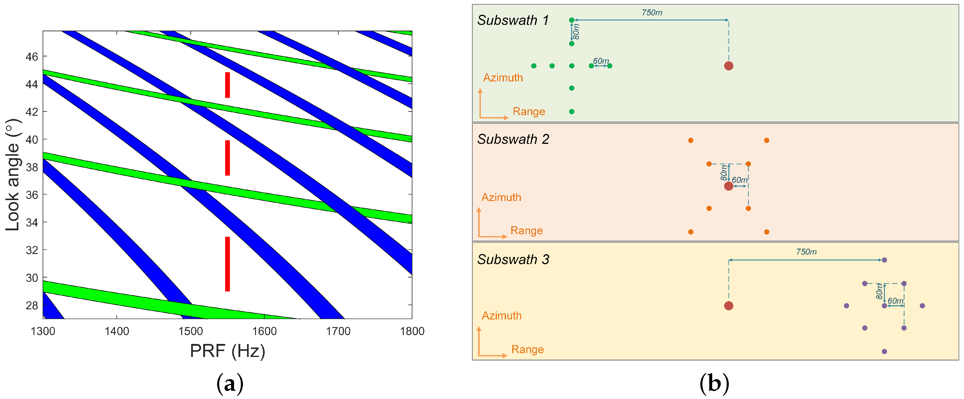
| PRF (Hz) | 1550 |
| Look angle of antenna normal direction () | 30 |
| Index | PRF (Hz) | Look Angle () |
|---|---|---|
| 1 | 1550 | [28.97, 32.92] |
| 2 | 1550 | [37.35, 39.91] |
| 3 | 1550 | [42.97, 44.82] |
| Beamformer | Desired | Interference Subswath | ||
|---|---|---|---|---|
| Subswath | 1 | 2 | 3 | |
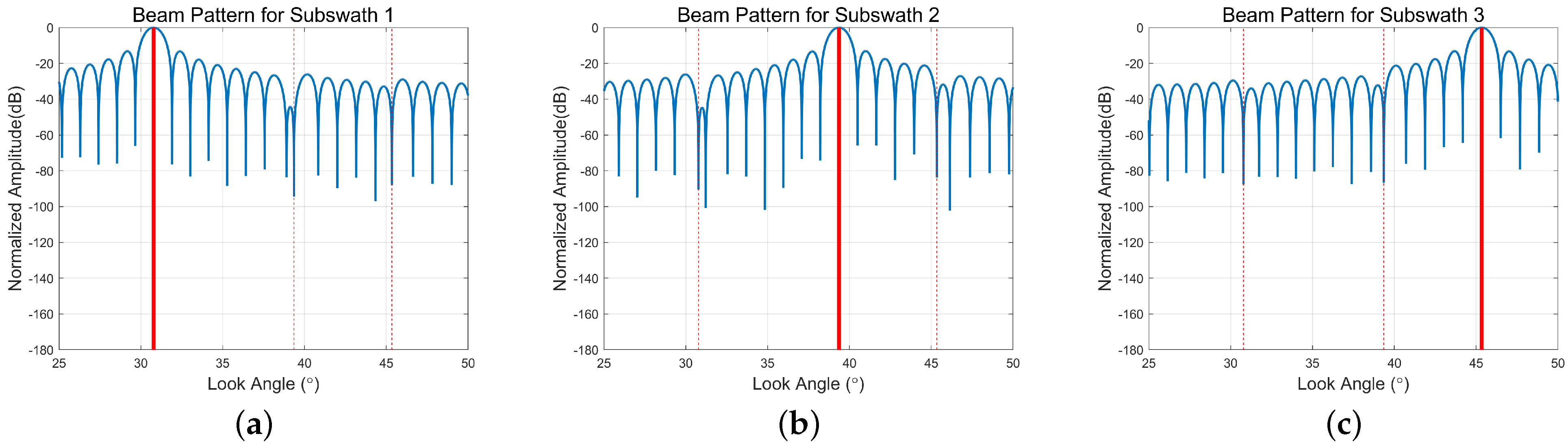
| LCMV | 1 | \ | −55.36 dB | −59.70 dB |
| 2 | −47.72 dB | \ | −66.33 dB | |
| 3 | −23.33 dB | −54.10 dB | \ | |
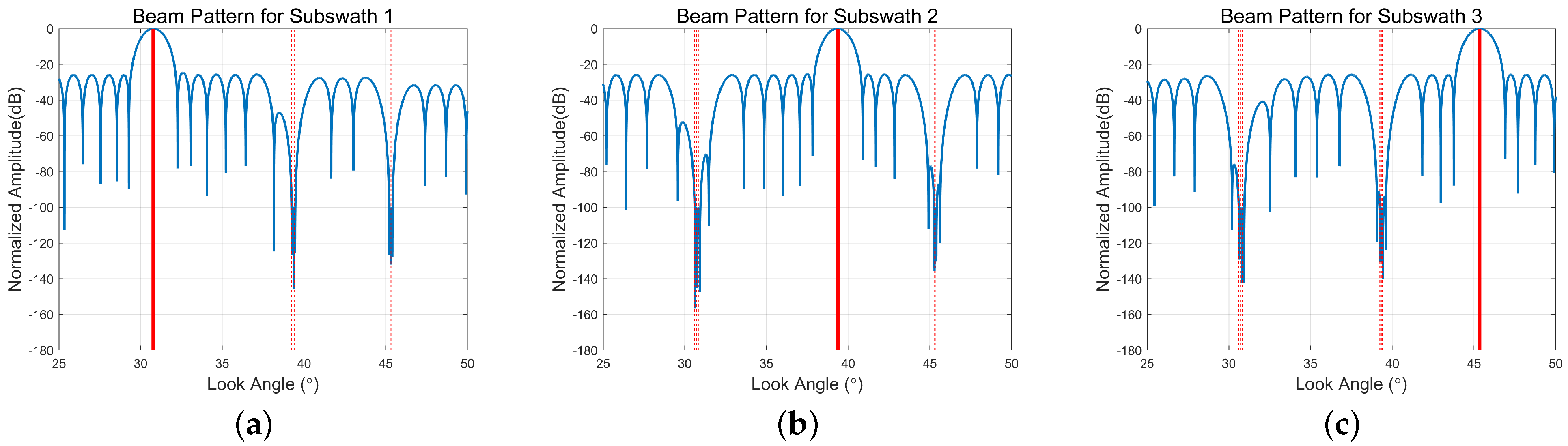
| SOCP | 1 | \ | −55.36 dB | −59.70 dB |
| 2 | −62.96 dB | \ | −66.37 dB | |
| 3 | −62.45 dB | −58.03 dB | \ | |
| Parameter | Value |
|---|---|
| Height (m) | 4200 |
| Platform velocity (m/s) | 80 |
| Carrier frequency (GHz) | 9.6 |
| Signal bandwidth (MHz) | 500 |
| Pulse duration (s) | 10 |
| Oversampling rate | 1.2 |
| Antenna height (m) | 0.32 |
| Antenna length (m) | 0.496 |
| Numbers of channels | 16 |
| PRF (Hz) | 1500 |
| Look angle of antenna normal direction () | 65 |
Publisher’s Note: MDPI stays neutral with regard to jurisdictional claims in published maps and institutional affiliations. |
© 2022 by the authors. Licensee MDPI, Basel, Switzerland. This article is an open access article distributed under the terms and conditions of the Creative Commons Attribution (CC BY) license (https://creativecommons.org/licenses/by/4.0/).
Share and Cite
Han, S.; Deng, Y.; Wang, W.; Zhao, Q.; Qiu, J.; Zhang, Y.; Chen, Z. A Novel Echo Separation Scheme for Space-Time Waveform-Encoding SAR Based on the Second-Order Cone Programming (SOCP) Beamformer. Remote Sens. 2022, 14, 5888. https://doi.org/10.3390/rs14225888
Han S, Deng Y, Wang W, Zhao Q, Qiu J, Zhang Y, Chen Z. A Novel Echo Separation Scheme for Space-Time Waveform-Encoding SAR Based on the Second-Order Cone Programming (SOCP) Beamformer. Remote Sensing. 2022; 14(22):5888. https://doi.org/10.3390/rs14225888
Chicago/Turabian StyleHan, Shuo, Yunkai Deng, Wei Wang, Qingchao Zhao, Jinsong Qiu, Yongwei Zhang, and Zhen Chen. 2022. "A Novel Echo Separation Scheme for Space-Time Waveform-Encoding SAR Based on the Second-Order Cone Programming (SOCP) Beamformer" Remote Sensing 14, no. 22: 5888. https://doi.org/10.3390/rs14225888
APA StyleHan, S., Deng, Y., Wang, W., Zhao, Q., Qiu, J., Zhang, Y., & Chen, Z. (2022). A Novel Echo Separation Scheme for Space-Time Waveform-Encoding SAR Based on the Second-Order Cone Programming (SOCP) Beamformer. Remote Sensing, 14(22), 5888. https://doi.org/10.3390/rs14225888