A Multi-Channel Descriptor for LiDAR-Based Loop Closure Detection and Its Application

Abstract

Simultaneous localization and mapping (SLAM) algorithm is a prerequisite for unmanned ground vehicle (UGV) localization, path planning, and navigation, which includes two essential components: frontend odometry and backend optimization. Frontend odometry tends to amplify the cumulative error continuously, leading to ghosting and drifting on the mapping results. However, loop closure detection (LCD) can be used to address this technical issue by significantly eliminating the cumulative error. The existing LCD methods decide whether a loop exists by constructing local or global descriptors and calculating the similarity between descriptors, which attaches great importance to the design of discriminative descriptors and effective similarity measurement mechanisms. In this paper, we first propose novel multi-channel descriptors (CMCD) to alleviate the lack of point cloud single information in the discriminative power of scene description. The distance, height, and intensity information of the point cloud is encoded into three independent channels of the shadow-casting region (bin) and then compressed it into a two-dimensional global descriptor. Next, an ORB-based dynamic threshold feature extraction algorithm (DTORB) is designed using objective 2D descriptors to describe the distributions of global and local point clouds. Then, a DTORB-based similarity measurement method is designed using the rotation-invariance and visualization characteristic of descriptor features to overcome the subjective tendency of the constant threshold ORB algorithm in descriptor feature extraction. Finally, verification is performed over KITTI odometry sequences and the campus datasets of Jilin University collected by us. The experimental results demonstrate the superior performance of our method to the state-of-the-art approaches.

1. Introduction

SLAM [1] is a key technology in the field of UGV, which can provide a prior map for UGV to perform the positioning function. The SLAM system [2,3,4] estimates the poses of vehicles within a certain period of time through the continuous data collected by the sensors and builds incremental maps via these estimated poses to achieve the goals of self-orientation and mapping. Undoubtedly, accurate estimation of poses is a key link in the whole process. The higher the accuracy of pose estimation, the higher the mapping quality. However, the traditional pose estimation methods that rely only on the interframe matching of the odometer are prone to the problem of error accumulation. The estimated trajectory of a system in long-time operation is bound to deviate significantly from the actual moving trajectory. These drift errors can be corrected by additional information provided by the LCD algorithm [5,6], which can recognize the revisited region by building a new constraint relationship between the current and historical frames to supplement the inter-frame pose estimation. However, existing LCD solutions, including vision and light detection and ranging (LiDAR) based methods, remain defective in some aspects and cannot meet the demands of practical applications.

The existing vision-based LCD algorithms mainly adopt the strategy of combining Oriented FAST and rotated BRIEF (ORB) bag-of-words model [7] and Random Sample Consensus (RANSAC) [8,9] method. These LCD methods have the advantages of high retrieval efficiency and rotation invariance regardless of the changes in viewpoints. However, the bag-of-words database must be built in advance, and the subsequent candidate verification steps are cumbersome. In addition, the performance of these vision-based methods is susceptible to the factors such as light, weather, and perspective. Compared with vision-based methods, common radar LCD methods involve one more step to project point clouds into a 2D image. The main difficulty of these methods is manifested in how to design descriptors and ensure the similarity score calculation is rotation-invariant. Scan Context (SC) [10,11] exploits a bird-eye view (BEV) to project 3D point clouds into an expanded image. Though maximum height and intensity information reflect the environmental information condition to some extent, they are both low-dimensional descriptors generated according to the single features of point clouds at the loss of much information contained in point clouds. The discriminative power of these descriptors weakens in the case of many similar buildings in the data collection process. Moreover, this coding approach transforms the rotational change of sensors into the column sequence change of images so that the traditional scheme of extracting rotation-invariant features from images is no longer applicable. It is because the change relation between columns in the descriptors via brute-force retrieval is essential before calculating the similarity. Evidently, this method has enormous room for improvement. Shan [12] used LiDAR with 128 channels to generate a ring view of the environment based on the intensity information. Then an ORB descriptor and RANSAC combined method was successfully introduced into the LiDAR-based LCD. Despite the success of this method in applying the traditional image feature extraction method to the LiDAR-based method, the process of extracting image features is heavily dependent on high-resolution LiDAR; otherwise, it would be difficult for descriptors generated on low-resolution LiDAR to acquire valid features.

According to the above analysis, the existing LCD algorithms remain open to the following problems: (1) The descriptors constructed via the single information of point clouds are lacking in the discriminative power of scene description; (2) the constant threshold ORB algorithm is hard to extract descriptor features effectively; (3) the common similarity calculation methods are sensitive to rotation and poor in interpretability, leading to misdetection or omitted detection of loop closure. To address these issues, this paper begins by bringing forth a method for the construction of multi-channel descriptors (CMCD), with the distance, height, and intensity information of point clouds introduced, coded into three separate channels in the projection subregions (bins), and then compressed into 2D global descriptors. Next, an ORB-based dynamic threshold feature extraction algorithm, DTORB, is designed. This algorithm calculates the dynamic threshold according to the standard deviation of objective global pixel values and the difference between pixel values within local areas and then extracts the features of descriptors according to the dynamic threshold. Finally, a DTORB-based similarity measurement method is proposed. This approach transforms the problem of similarity between point clouds into the problem of similarity between images and calculates the similarity score derived from the Hamming distance between these features by matching the DTORB features of two images. This process is also visualized. The main contributions of our paper can be summarized as below:

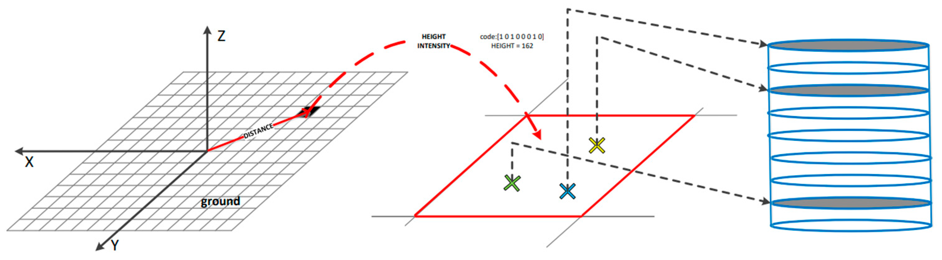
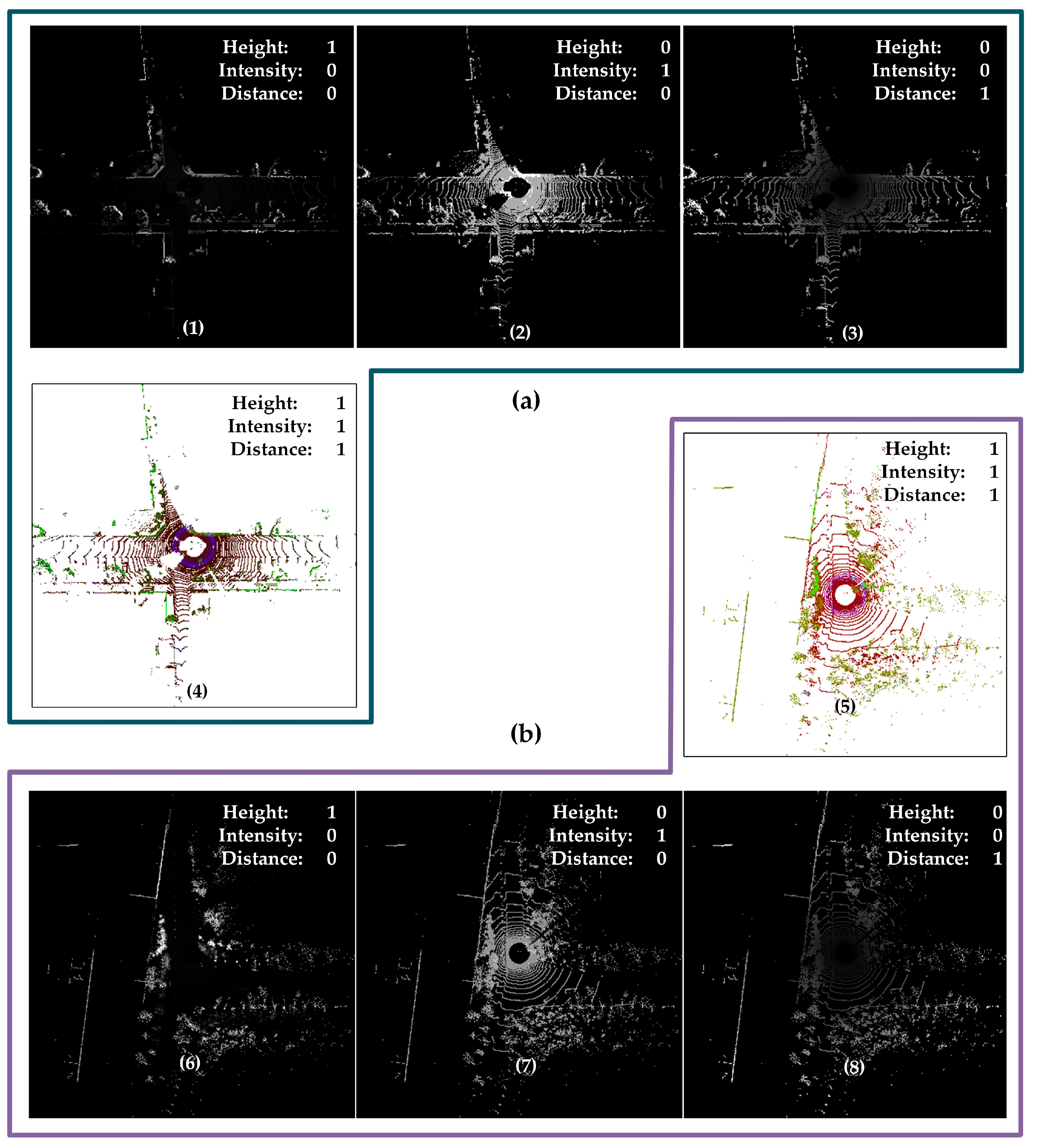
• The method for CMCD: A novel CMCD method is proposed to resolve the lack of point clouds in the discriminative power of scene description. It enhances the discriminative power of descriptors and mitigates the effect of abnormal pixel values in a single channel on subsequent feature screening by synthesizing the distance, height, and intensity features of point clouds.
• The feature extraction algorithm DTORB: The feature extraction algorithm DTORB is designed to get rid of the subjective tendency of the constant threshold ORB algorithm in extracting descriptor features. A dynamic threshold is designed to screen features via the objective global and local distributions of point clouds to ensure high-quality features can still be extracted from the three-channel images generated using point clouds. Meanwhile, the rotation-invariance property of ORB features guarantees DTORB features are also rotation-invariant.
• A rotation-invariant similarity measurement method is developed to figure out the similarity score between descriptors by calculating the Hamming distance between matched features. Its theoretical basis is also visualized.
• A comprehensive evaluation of our solution is made over the KITTI odometry sequences with a 64-beam LiDAR and the campus datasets of Jilin University collected by a 32-beam LiDAR, and the results demonstrate the validity of our proposed LCD method.

The remaining part of this paper is organized as follows: Section 2 reviews the existing LCD methods; Section 3 elaborates on our LCD algorithm, including the construction of multi-channel descriptors, determination of the loop candidate set, DTORB feature extraction, and similarity measurement; Section 4 displays the experimental results; Section 5 draws the conclusion. Figure 1 is a schematic of CMCD blocks for multi-channel descriptors.

2. Related Work

2.1. Vision-Based LCD

Existing LCD methods can generally be classified into vision-based and LiDAR-based solutions. Most common in vision-based LCD is the bag-of-words [8] model that builds a dictionary via the extracted image features and then a bag-of-words vector according to whether the feature appears in the image. Sivic et al. [13] were the first to use the bag-of-words model in the vision-based LCD task. They built a visual dictionary by discretizing the extracted image features to figure out the frequency of occurrence of different words describing different scenes and decide whether there existed a loop closure. Cummins [14] implemented LCD by combining Speeded Up Robust Features (SURF) [15] with a dependency tree to generate a bag-of-words model. Mur-Artal et al. [16] extracted ORB features with rotation invariance and scale invariance to construct a bag-of-words vector for LCD and used Random Sample Consensus (RANSAC) to eliminate mismatched loop frames. Dorian et al. [17] constructed a vocabulary tree of discrete binary descriptor space to accelerate the geometric verification process of the bag-of-words model. Liu et al. extracted the compact high-dimensional descriptors from single images and used PCA to reduce the dimensionality of LCD to boost computational efficiency. However, the images acquired using a camera by the vision-based LCD method are susceptible to changes in the environment, illumination, and perspective during loop detection, leading to insufficient accuracy of follow-up feature extraction and greatly affecting the performance of LCD.

2.2. LiDAR-Based LCD

The LiDAR-based LCD method has stronger adaptiveness to changes in the environment, illumination, and perspective and higher robustness, and can acquire rich information, such as 3D coordinates, distance, azimuthal angles, surface normal vector, and depth, from point clouds. The LiDAR-based LCD method can be further divided into two categories: one is to extract local or global descriptors directly from point clouds, and the other is to use the image as the intermediate representation.

The first category of methods lays a particular emphasis on extracting local or global descriptors directly from point clouds. ESF [18] constructs global descriptors of point clouds using three features: distance, angle, and area distributions. However, this solution overlooks the effects of rotation and translation. Rusu et al. [19] proposed the Fast Point Feature Histogram (FPFH), using the local normal lines of scanning points to construct a key point feature histogram to detect a loop, but the normal line information has high computational complexity and poor real-time performance. Bosse et al. [20] extracted Gestalt key points and descriptors from point clouds and used key point voting to identify positions. SegMatch et al. [21] segmented a point cloud into distinct elements, extracted features from each segmented result, and then matched the features by the deep learning method. PointNetVLAD [22] utilized PointNet [23] to extract features from point clouds and used NetVLAD [24] to generate global descriptors. All these above methods are poor in generalization as they need training with mass data.

The second category projects LiDAR point clouds onto the 2D plane(s) by means of dimensionality reduction and then solves the LCD problem using a 2D method. M2DP [25] projects point clouds onto multiple 2D planes and calculate the left and right singular vectors of each plane as global descriptors according to the density feature, but it overlooks the rotation problem. SC divides a BEV into several bins, each of which takes the maximum height to form SC descriptors in terms of the azimuthal angle and radial direction and adopts a two-stage search to detect a loop. Although the effect of LiDAR viewpoint changes is mitigated by brute-force matching, SC [10] is not ideal for dealing with rotation invariance. As an improvement over SC, ISC [26] constructs a global descriptor for the value assigned to each bin in the combination of point cloud density and geometrical information, using a two-stage layered recognition process for loop detection. Although making up for the detection error due to the maximum height merely used by SC, ISC still leaves the rotation invariance problem unresolved. To solve the brute-force matching problem of SC, IRIS [27] projects point clouds into a BEV and obtains a binary image through Log-Gabor filtering and threshold operation to search loop candidates. Although it has solved the rotation invariance problem, its effectiveness is unsatisfactory in practical application. BVMatch [28] constructs a maximum index map via the Log-Gabor filter to acquire the local descriptors of BEV Feature and then a bag-of-words vector for scene recognition. OverlapNet [29] uses range, normal vector, intensity, and semantic information to project point clouds into 2D images and adopts a Siamese neural network to estimate the overlapping ratio and relative yaw angle of the images and to ultimately complete loop closure detection and correction. However, such a deep learning-based method is weak in generalization and needs to undergo transfer training to be applied in specific scenarios with mass data and high computational complexity. Shan et al. [12] projected the point clouds of a 128-beam imaging-level LiDAR into an intensity map in the light of a point cloud sphere. Subsequently, they built a bag-of-words model to query for the loop candidate set by extracting ORB features from the image. This method has not only a high requirement on the equipment but also a certain requirement on the size of the bag-of-words model, needing to update the bag-of-words model whenever a new scene appears.

Our motivation in this paper is to introduce relevant methods of 2D LCD into 3D LCD tasks. The crux is to design a 3D-to-2D projection method, which requires considering the high fidelity of point cloud data on the one hand and whether the descriptors are consistent due to sensor viewpoint change on the other hand. Therefore, the method for CMCD, which is distinguished from the foregoing descriptors containing only the single features, is designed. The distribution, vertical structure, and reflection information of point clouds are made full use of to enhance the discriminative power of descriptors and reduce the interference of outliers occurring in the single information to follow-up feature extraction while saving the information content. The rotation invariance problem is approached by extracting DTORB features. Although our generated descriptors constitute a BEV, which might rotate with sensor viewpoint change, it remains possible for us to extract consistent features from the rotated image based on the rotation invariance of ORB descriptors. Finally, the similarity score of descriptors is obtained from the Hamming distance between matched features. In a visualized way, we displayed the extracted features and the matching condition between them, giving a visual presentation of the rationality of this method. The entire method proposed by us is distinguished from the LiDAR-based method using ORB features and from the vision-based methods. Having low requirements on the resolution of LiDAR, our method is applicable to both high- and low-beam LiDAR data. Our proposed method does not require the construction of dictionary vectors. Different from the bag-of-words model, our algorithm first extracts the retrieval vector of the descriptor. Then, based on this vector, the nearest 10-frame point cloud is retrieved from the KD tree. Next, the DTORB features of the descriptors corresponding to the current point cloud and candidate point cloud are extracted. Finally, the Hamming distance of matched features is calculated to score the similarity. Since the distances of DTORB features are computed directly, rather than calculating scores against the dictionary as in the bag-of-words model, there is no need to construct an appropriately sized dictionary in advance or update the dictionary as new scenes emerge.

3. Methods

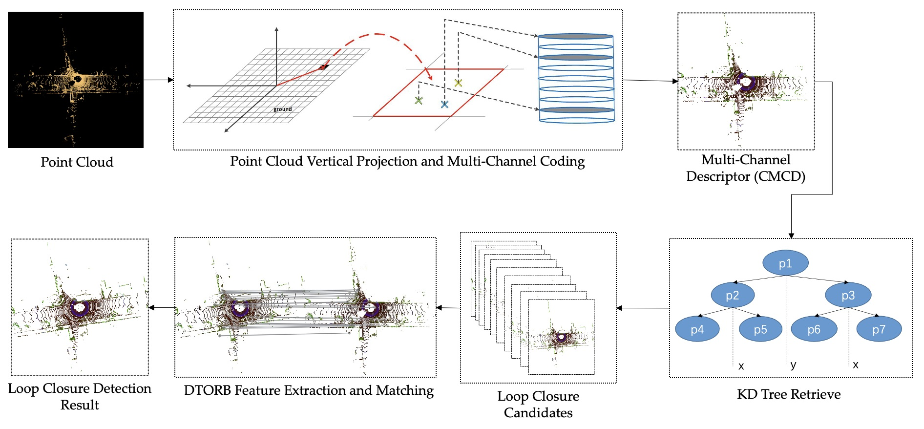
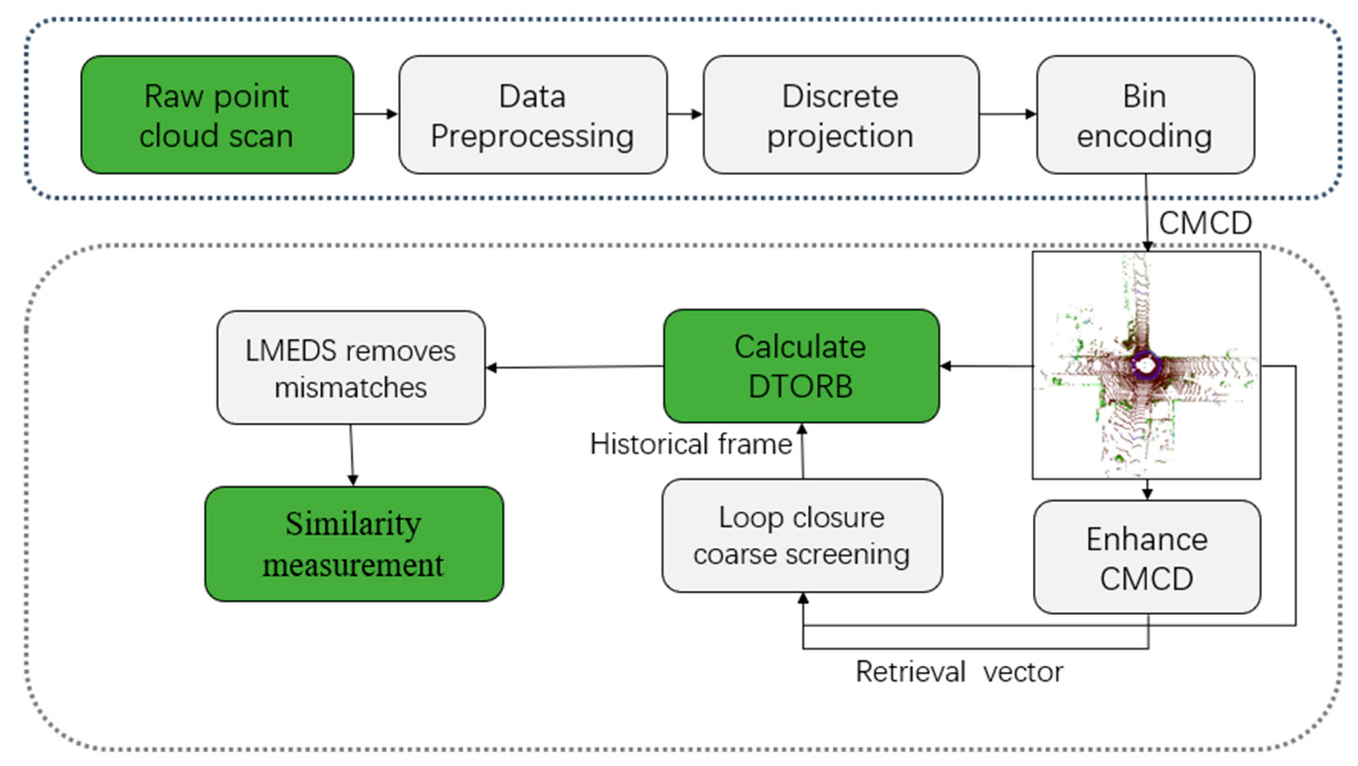
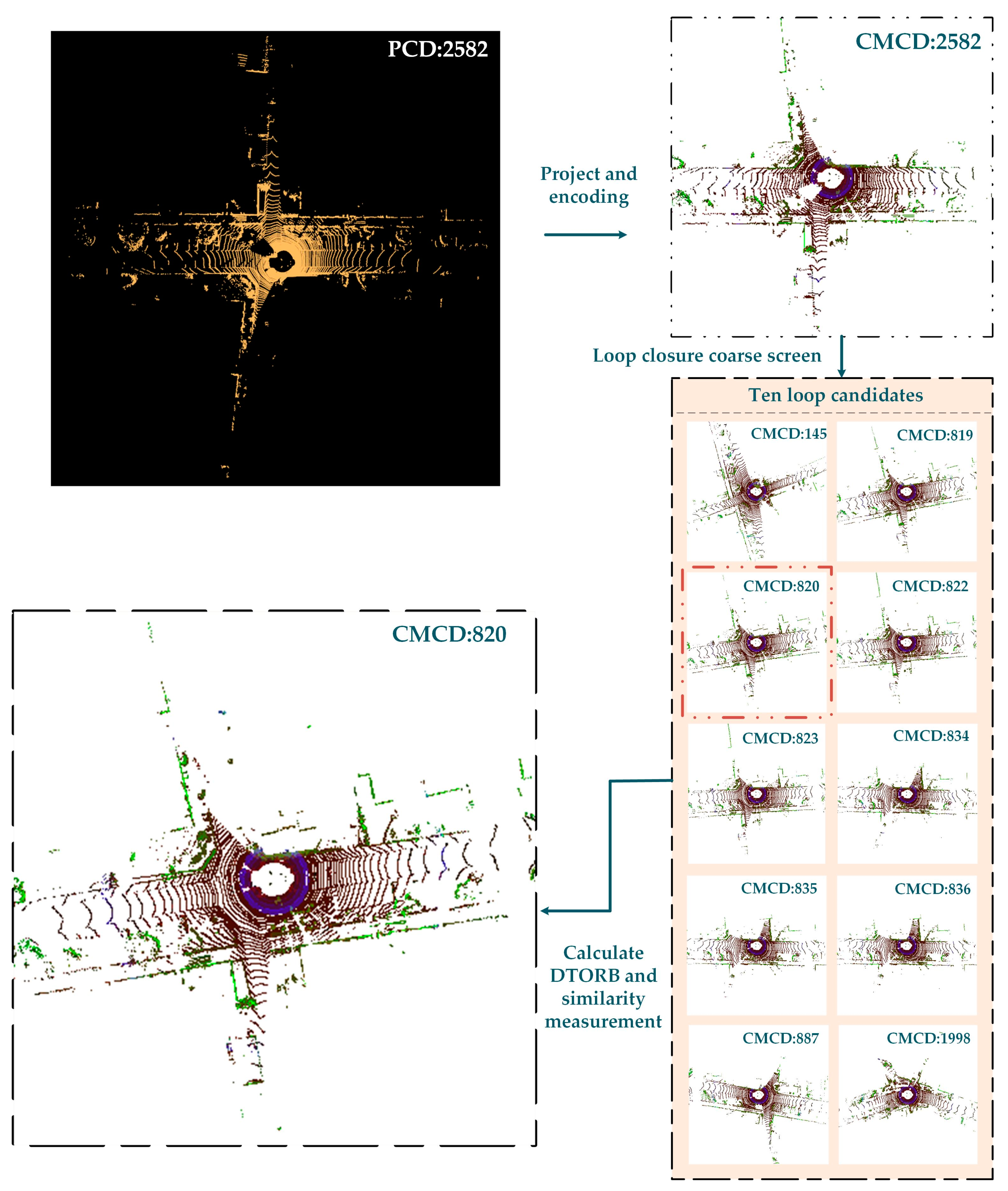
3.1. System Overview

This section introduces our solution in four major stages: construction of multi-channel descriptors, selection of loop candidates, DTORB feature extraction, and similarity measurement. The concrete pipeline of the procedure is shown in Figure 2. To start with, the point clouds are projected and encoded into multi-channel descriptors after undergoing data preprocessing. Next, possible loop candidates are selected by the descriptors. The first step is to calculate the translation-invariant retrieval vector and linear weighted distance for CMCD to get the loop candidate set of the current point clouds; the second step is to extract rotation-invariant DTORB features for the descriptors; the third step is to calculate the Hamming distance between matched rotation-invariant features as the similarity score and decide whether the two-frame point clouds are a loop-closing pair.

3.2. Construction of Multi-Channel Descriptors

Given a 3D point cloud P, project it vertically onto the $xOy$ plane of the sensor coordinate system. Select the square region with area $RANGEX\times RANGEY$ centered at Origin O as the region of interest (ROI). Segment ROI into $N_x$ × $N_y$ subregions with equal size, where $N_x$ and $N_y$ correspond to the number of blocks divided on each side of the square region, respectively, as shown in Figure 3. Each subregion at the row $i$ and the column $j$ is symbolized by $B_j^i$ for all point clouds in it. The row index and column index of this subregion are calculated by the following formulae:

$$P=\underset{iϵN_x,jϵN_y}{{\displaystyle \cup }}{B}_j^i$$

(1)

$$i=\frac{\frac{x\left(p\right)+RANGEX}{2}}{RANGEX}\times N_x$$

(2)

$$j=\frac{\frac{y\left(p\right)+RANGEY}{2}}{RANGEY}\times N_y$$

(3)

where p denotes a point among the point clouds within the current subregion $B_j^i$; $x\left(p\right)$ and $y\left(p\right)$ represent the x- and y-coordinate information about point $p$, respectively; $RANGEX$ and $RANGEY$ are offsets which ensure the row index and column index of point cloud block $B_j^i$ fall within the range of positive integers. In this paper, we set $RANGEX=120 \mathrm{m}$, $RANGEY=120 \mathrm{m}$, $N_x=160$, and $N_y=160$. At this point, the size of the scanning region in real scenes corresponding to each subregion is 0.75 m × 0.75 m.

A one-frame point cloud is divided into several subregions after undergoing the above partitioning. Traditional descriptors mostly adopt the single features of point clouds, but it would be difficult to make a distinction between different point clouds when part of the rich information contained is used. Moreover, the existing descriptors are hard to extract traditional image features. So, we designed multi-channel descriptors CMCD, using multiple features to construct descriptors and represent point clouds by multi-channel means. Referring to the RGB color pattern of images, we set three information channels for each subregion, which were assigned values in terms of the distance, height, and intensity features of the point clouds within that subregion.

The value assigned to the first channel is the maximum distance $R_{B_j^i}$ between the points in $B_j^i$ and Origin $O$ of the sensor coordinate system, as calculated by the formula:

$$R_{B_j^i}=max\sqrt{x{\left(p\right)}^2+y{\left(p\right)}^2},pϵB_j^i$$

(4)

The value assigned to the second channel is the height information coding result $H_{B_j^i}$ for the points in $B_j^i$. We encoded the height values into octal codes and then converted them into decimal numbers as the final $H_{B_j^i}$ for all points within a subregion by referring to IRSI [27]. The specific way of height coding is described as below: For the set of point clouds within each subregion, firstly, sort them by height. Then, linearly discretize them into eight bins (not each bin has points, and the value of the bins with points is 1, whereas the value of those without is 0) so as to obtain 8-bit binary codes for the height information. Finally, convert them into decimal numbers, as shown in Figure 3.

The value assigned to the third channel is the intensity information coding result $I_{B_j^i}$ for the points in $B_j^i$. The intensity information is encoded into the final result $I_{B_j^i}$ in the same way as the height information.

Through partitioning and coding, and then compressing the codes into grayscale global descriptors containing rich information, a point cloud is represented as a multi-channel descriptor CMCD, as shown in Figure 3. A CMCD reveals the distributional structure, vertical structure, and reflection information of the ambient and can accurately discriminate different scenes while reducing the interference of outliers to follow-up feature extraction.

3.3. Selection of Loop Candidates

To speed up the retrieval, the translation-invariant search vector [10] is designed by which to build a fast-retrieving KD tree [30]. Furthermore, the linear weighted distance is devised by performing nearest-neighbor retrieval to find the most similar historical point cloud to the current ones and construct a loop candidate point cloud set. To follow the concrete steps, the CMCD is flipped in the x-direction and y-direction, respectively, to get the enhanced descriptors; the L1-norms of all rows are taken for the original and enhanced descriptors and added up to get a 160-dimensional original retrieval vector. The enhanced descriptors ensure the most similar candidates are still retrievable when the sensor viewpoint is reversed. The retrieval vector calculated in the x-direction is endowed with translation invariance, ensuring the nearest neighbors are retrievable in the event of horizontal translation. Meanwhile, for the retrieval vector stored in the KD tree to be more representative, and to reduce dimensionality and speed up the retrieval. The principal component analysis (PCA) [31] is conducted on the original retrieval vector to derive an eigenmatrix $Q$ by which to reduce the dimensionality of the original retrieval vector. The new retrieval vector after dimensionality reduction is stored in the KD tree for retrieving historical frames. The new retrieval vector $Query$ is calculated by the formula:

$$Query=\left(\mu \left(I^1\right),\dots ,\mu \left(I^i\right)\right)$$

(5)

$$\mu (I^i)=( {\displaystyle \sum }_{j=0}^{159}(L(I_j^i)+L({I_x}_j^i)+L({I_y}_j^i)))\times Q$$

(6)

where $I_j^i$ is the pixel value of the subregion corresponding to the original descriptors, $I_x{}_j^i$ and $I_y{}_j^i$ are pixel values of the subregion corresponding to the enhanced descriptors; $i$ and $j$ are the row and column indexes of CMCD, respectively; $L()$ signifies calculating the L1-norm of the element within the parentheses; $Q$ is the eigenmatrix obtained after PCA processing.

To speed up the retrieval of the KD tree and meet the real-time performance requirement of LCD, the linear combination of the Manhattan distance $D_1$, and the chessboard distance $D_{\infty }$ with low computational complexity is selected instead of the Euclidean distance as the criterion for KD tree retrieval. The Manhattan distance $D_1$ is calculated by the formula:

$$D_1\left(x,y\right)={\displaystyle \sum }_{i=1}^n\left|x_i-y_i\right|$$

(7)

The chessboard distance $D_{\infty }$ is calculated by the formula:

$$D_{\infty }=\underset{1\le i\le n}{\max }\left\{\left|x_i-y_i\right|\right\}$$

(8)

The linear combination is calculated by the formula below:

$$D=\omega \times (D_1+D_{\infty })$$

(9)

where the weight $\omega =0.5$.

The retrieval vector of CMCD is then by Formula (5) and stored in the KD tree. The ten most similar historical point clouds, of which the IDs are in a candidate set of loop-closing pairs, to the current point clouds are retrieved by Formula (9). The results of the selection of loop candidates are shown in Figure 4. We project and encode the point cloud at frame 2582 of KITTI-05 to obtain the descriptor CMCD. Then we calculate the retrieval vector for CMCD according to the formula and quickly retrieve the ten most similar loop candidates from the KD tree according to the linear combination distance. The frame IDs of the ten most similar loop candidates are 145, 819, 820, 822, 823, 834, 835, 836, 887, and 1998, respectively.

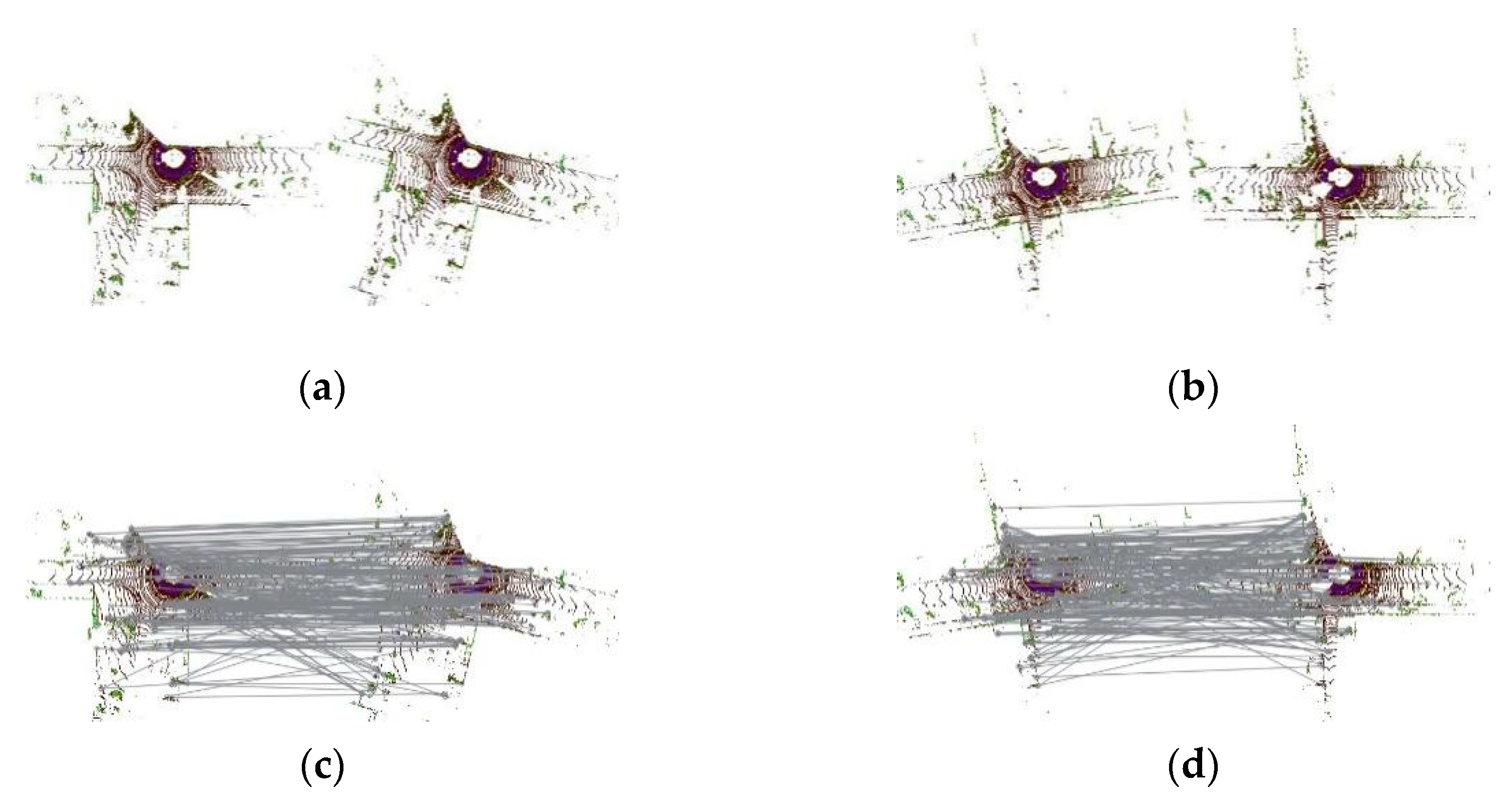
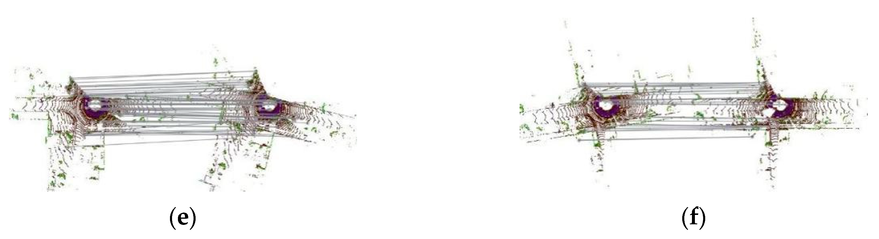
3.4. DTORB Feature Extraction Algorithm

Considering that LiDAR data undergo viewpoint change or horizontal shift in the revisited place, it is necessary to extract rotation-invariant features from the current CMCD and those corresponding to the loop candidate set. The ORB feature extraction algorithm [7] can extract rotation-invariant and scale-invariant features from the image to meet our requirements. However, given that the ORB algorithm is applied in traditional images, it would be too subjective to screen features using a fixed threshold, and it would deviate from the intended effect if used directly to extract the rotation-invariant features of CMCD. Therefore, the aspect of feature extraction of ORB algorithm by designing a dynamic threshold feature extraction and description algorithm DTORB. This algorithm sets a global threshold via the degree of dispersion of the pixel values of the entire descriptor, as well as a local threshold via the difference between the pixel values within a local region, according to the thought of the variable-threshold method. The global and local thresholds are integrated to calculate the dynamic threshold to extract feature points discriminatively. The specific procedure is described as follows:

DTORB adopts a three-layer image pyramid to obtain CMCD with distinct resolutions after graying the image and then extracting FAST [32] feature points for each CMCD using the dynamic threshold. Considering the degree of dispersion of pixel values of the entire descriptor, the dynamic global threshold of the entire CMCD is first calculated. To avoid the effect of outliers on the threshold, the standard deviation of grayscale values excluding the maximum and the minimum is taken as the global threshold ${\alpha }_t$:

$${\alpha }_t=\sqrt{\frac{{\sum }_{i=1}^N{(I_i-I_m)}^2}{N}}$$

(10)

where $N$ is the total number of points in the image; $I_i$ is the grayscale value of each point; $I_m$ is the mean of grayscale values of the remaining points after excluding the maximum and minimum grayscale values.

Considering the degree of deviation of data within the neighborhood, the dynamic local threshold ${\beta }_t$ of the neighborhood encompassing each point is calculated by the following formula:

$${\beta }_t=k_1\times \frac{I_{max}-I_{min}}{I_m}$$

(11)

where $I_{max}$ and $I_{min}$ are the maximum and minimum grayscale values, respectively; $I_m$ is the mean of grayscale values of the 14 remaining points after excluding $I_{max}$ and $I_{min}$; $k_1$ is typically taken as 2–5.

The final dynamic threshold of feature points is selected as

$${\theta }_t=k\times {\alpha }_t+\left(1-k\right)\times {\beta }_t$$

(12)

where $k$ is typically taken as 0.5–1; ${\alpha }_t$ is the global dynamic threshold; ${\beta }_t$ is the local dynamic threshold.

Feature points are extracted by the following formula depending on the dynamic threshold ${\theta }_t$:

$$f\left(I_x,I_p\right)=\left\{\begin{array}{c}1,\left|I_x-I_p\right|\ge {\theta }_t\\ 0,\left|I_x-I_p\right|<{\theta }_t\end{array}\right.$$

(13)

$$N={\displaystyle \sum }_{x\in \left[1,16\right]}f\left(I_x,I_p\right)$$

(14)

where $I_x$ represents the grayscale value of the current point; $I_p$ represents the grayscale value of a neighborhood point, which is considered a feature point when $N$ ranges from 9 to 12.

After extracting FAST feature points according to the dynamic threshold, the follow-up steps of ORB are adopted for feature extraction. With the vector direction from the geometrical center to the center of mass of the feature point found within the feature point’s neighborhood as the feature point’s principal direction, the BRIEF [33] algorithm at the second stage of ORB is used to describe the feature point to acquire the rotation-invariant features of CMCD.

3.5. Similarity Measurement

At the stage of similarity measurement, the rotation-invariant features are first calculated for the current CMCD, and so are those corresponding to the loop candidate set by the DTORB feature extraction algorithm. Next, the distance between features is calculated after the mismatched ones are eliminated to decide whether the two-frame point clouds are a loop-closing pair. Since the rotation-invariant features are in binary form, the matching point between two features is first searched for, and then the Hamming distance between matched feature points is calculated for similarity measurement. The distance between feature points is calculated as follows:

$$d\left(des{c}_1,des{c}_2\right)={\displaystyle \sum }_{i=1}^{256}(x_i\oplus y_i)$$

(15)

where $des{c}_1$ and $des{c}_2$ are binary representations for two feature points, and $des{c}_1=[x_1,x_2,\dots ,x_{256}]$, $des{c}_{c2}=\left[y_1,y_2,\dots ,y_{256}\right]$; $\oplus$ denotes XOR operation; the values of x and y are 0 or 1.

At the feature point matching stage of rotation-invariant features, LMEDS [34] method is adopted to eliminate mismatched points to avoid their effect on the matching precision. This algorithm is sensitive to Gaussian noise, while DTORB has processed the CMCD image with Gaussian Blur before calculating features, so LMEDS is suitable for eliminating mismatched points after extracting features by DTORB, which delivers high precision and robustness. After mismatched points are eliminated, the distance between two rotation-invariant features is calculated as follows:

$$\mathrm{D}\left(DES{C}_{\mathrm{q}},DES{C}_c\right)=\frac{1}{N_k}{\displaystyle \sum }_{i=1}^{N_k}d$$

(16)

where $DES{C}_q$ and $DES{C}_c$ are rotation-invariant features of the current CMCD and historical CMCD; $N_k$ is the number of matched points; $d$ is the Hamming distance between matched feature points (See Formula (13)).

When the distance between rotation-invariant features is smaller than or equal to the given threshold, the two CMCDs are similar, and the corresponding two-frame point clouds are a loop-closing pair. For the loop candidate set obtained at the rough screening stage of loops, the distances between the rotation-invariant features of the current CMCD and each candidate CMCDs are calculated, and the candidate point cloud with the minimum distance is taken as the LCD result of the current point clouds, as formulated below:

$$c^{*}={}_{c_{k\in C}}{}^{argmin}D\left(DES{C}_q,DES{C}_{c_k}\right),s.t D<\tau$$

(17)

where $C$ is the index of the nearest candidate point cloud retrieved by the KD tree; $\tau$ is the given acceptance threshold, typically taken as 0.4–0.56; $c^{*}$ is the index of the most similar point cloud among the candidate point clouds to the current ones. These two-frame point clouds are a loop-closing pair. Feature matching is visualized in Figure 5:

4. Results

In this section, our algorithm is verified by comparative experiments with four common algorithms in LCD: SC [10], ISC [26], M2DP [25], and ESF [18]. The codes for SC [35], ISC [36], and M2DP [37] algorithms are downloadable from the author’s website, while ESF [38] algorithm is implemented in the point cloud library (PCL). The entire point cloud is deemed as a reference point, like the center of mass, of which the ESF descriptors are figured out to represent the frame of point clouds. All experiments are done on the same computer with OS Ubuntu20.04, 3.07 GHz frequency, CPU Intel X5675, and 16 GB memory.

4.1. Datasets

All experiments were done over four KITTI odometry sequences [39], and four datasets were collected on the campus of Jilin University. The datasets adopted by us are diversified, e.g., the diverse types of 3D LiDAR sensors (Velodyne HDL-64E with 64 beams and Velodyne HDL-32E with 32 beams) and of loop closure (both obverse and reverse loop closures). The KITTI odometry sequences are obtained by Velodyne HDL-64E mounted on vehicles, providing indexed scans and widely used in SLAM and LCD. Four sequences (00, 02, 05, and 06) are selected with loops among the 11 KITTI odometry sequences with ground truth for loop closure verification. The sequence KITTI-00 consists of 4541 frames of point clouds in total, with five segments of obverse loop closure; the sequence KITTI-02 consists of 4661 frames of point clouds in total, with two segments of obverse loop closure and one segment of reverse loop closure; the sequence KITTI-05 consists of 2761 frames of point clouds in total, with three segments of obverse loop closure; the sequence KITTI-06 has one segment of obverse loop closure.

Multiple segments of data with obverse and reverse loop closures are collected from the campus of Jilin University. The data are acquired by the devices 32-beam LiDAR Velodyne HDL-32E and inertial navigator NovAtel NPOS220S erected on Volkswagen Tiguan, with the vehicle’s speed maintained at about 30 km/h. Four scenes, jlu00, jlu01, jlu02, and jlu03, with distinct scales, are selected from our datasets to validate our method. Among them, jlu00 has 4626 frames, with two segments of obverse loop closure and one segment of reverse loop closure; jlu01 has 1262 frames in total, with one segment of obverse loop closure; jlu02 has 3894 frames in total, with one segment of obverse loop closure and one segment of reverse loop closure; jlu03 has 6190 frames in total, with one segment of obverse loop closure.

4.2. Experimental Settings

To obtain the actual precision rate and recall rate, the ground truth pose distance between the query and the matched frame is set as the criterion for loop detection. If the distance is smaller than 4 m, then the loop is considered true positive. To avoid matching with adjacent point clouds, no similarity judgment is made for the previous 50 frames and the next 50 frames to the current frame. Each frame of point clouds is projected into CMCD, the DTORB features are calculated after the rough screening by the KD tree, and the similarity between point clouds is measured according to the distance between features. Next, our parameters are optimized over the KITTI odometry sequences, and the distance threshold is continuously improved to accurately screen loop frames. In this paper, the parameters of CMCD are set as follows: the size of CMCD = 160 × 160, range of point cloud selection = 120 m × 120 m, dimension of the retrieval vector stored in the KD tree = 120, number of the nearest neighbors retrieved by the KD tree = 10. In SC, the number of the nearest neighbors retrieved by the KD tree is set as 10, the number of bins as 20 × 60, and the maximum radius as 80 m. In ISC, the number of bins is set as 20 × 90, and the maximum radius is set as 60 m. There is no parameter to set in ESF. In M2DP, the number of bins per 2D plane is set as 8 × 16, and the number of 2D planes to use is set as 4 × 16. These parameters are set according to the open-source code and the paper.

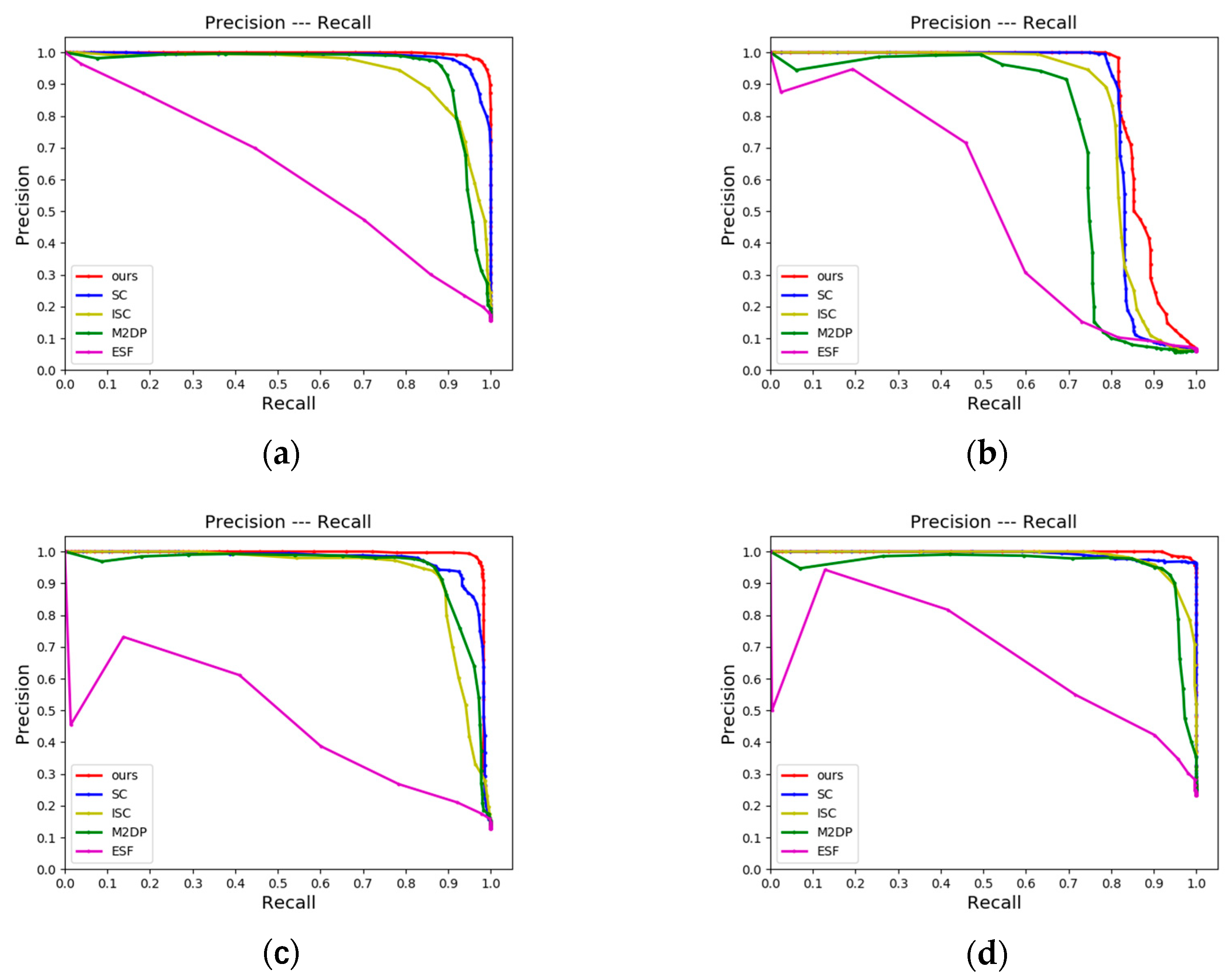
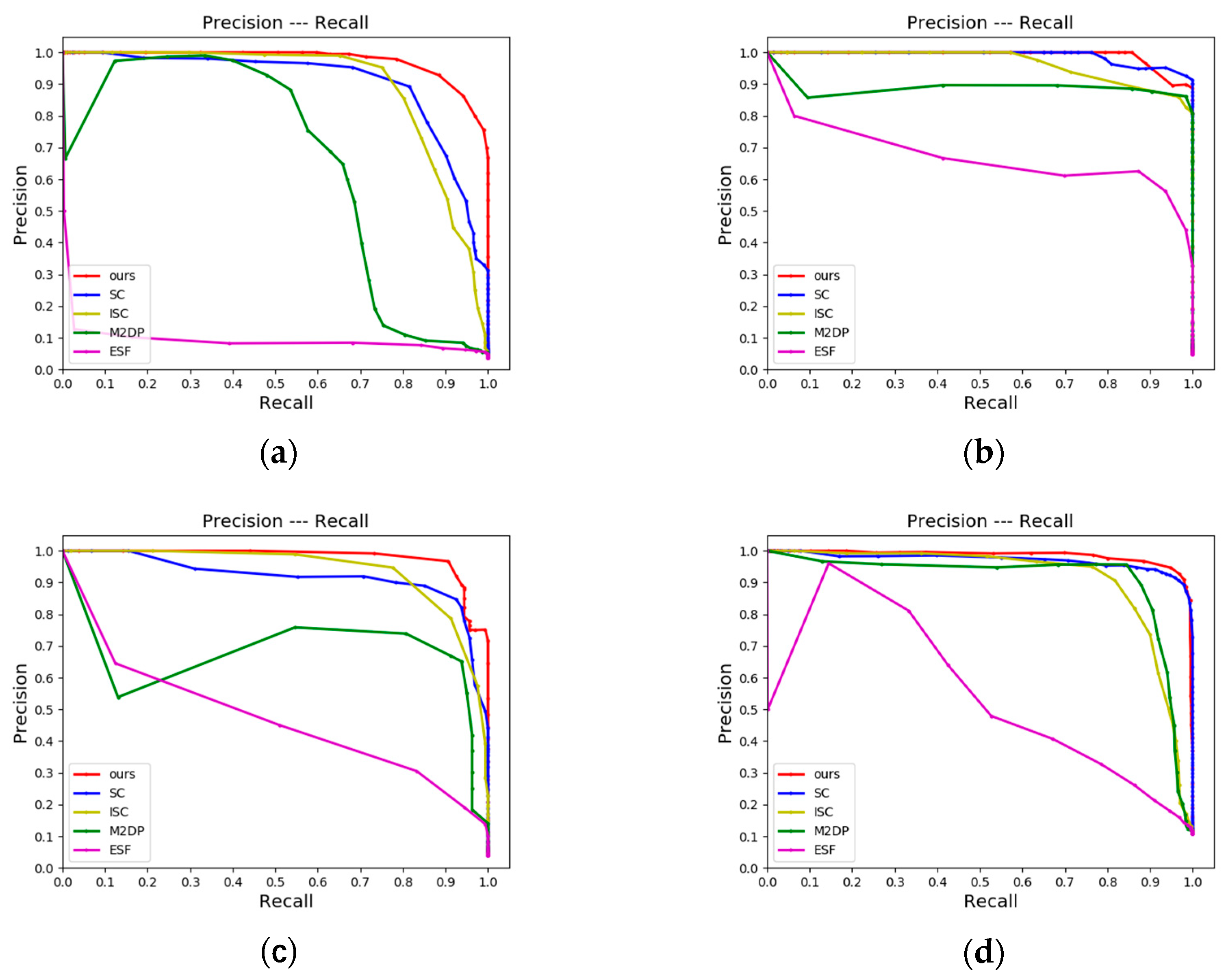
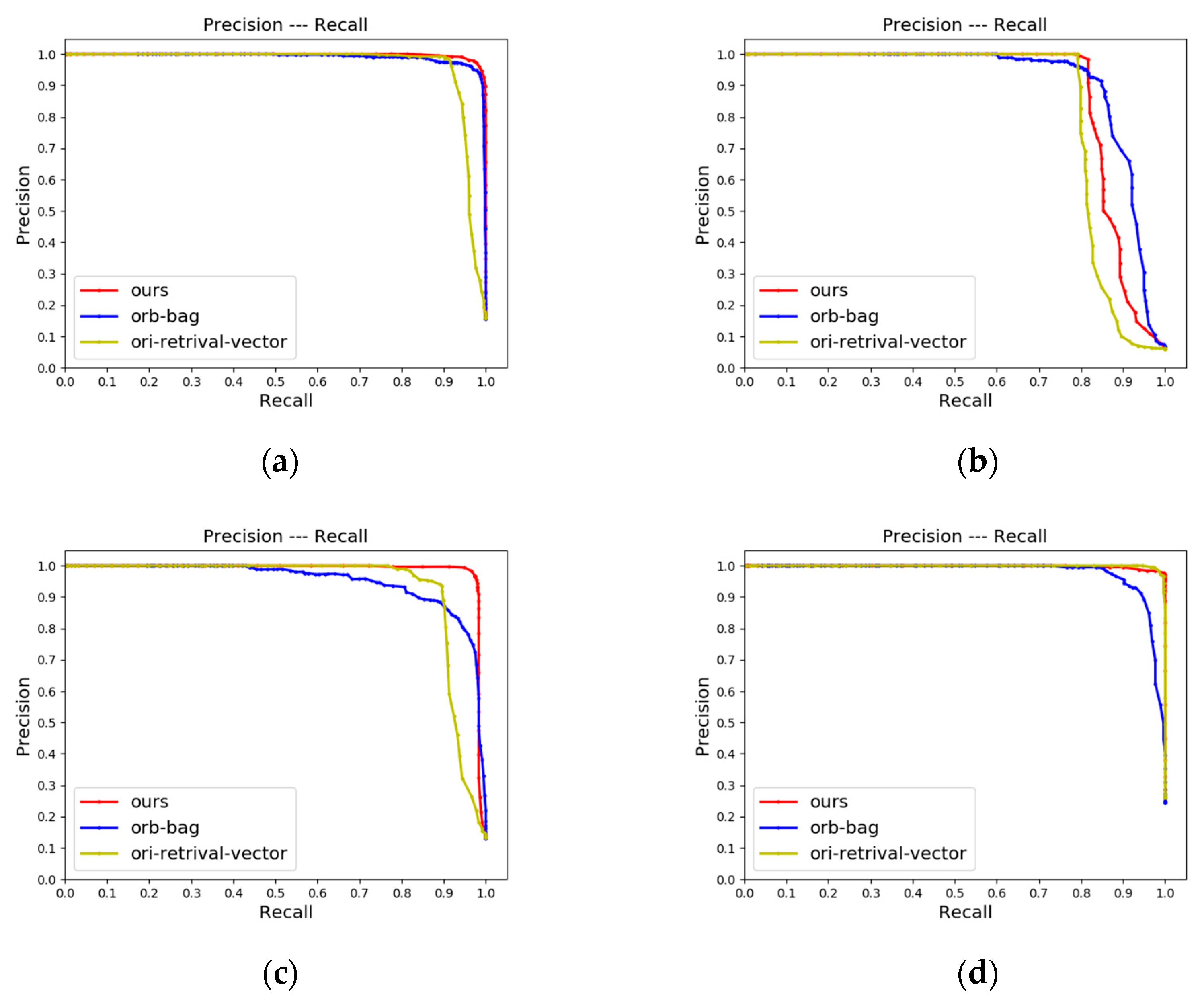
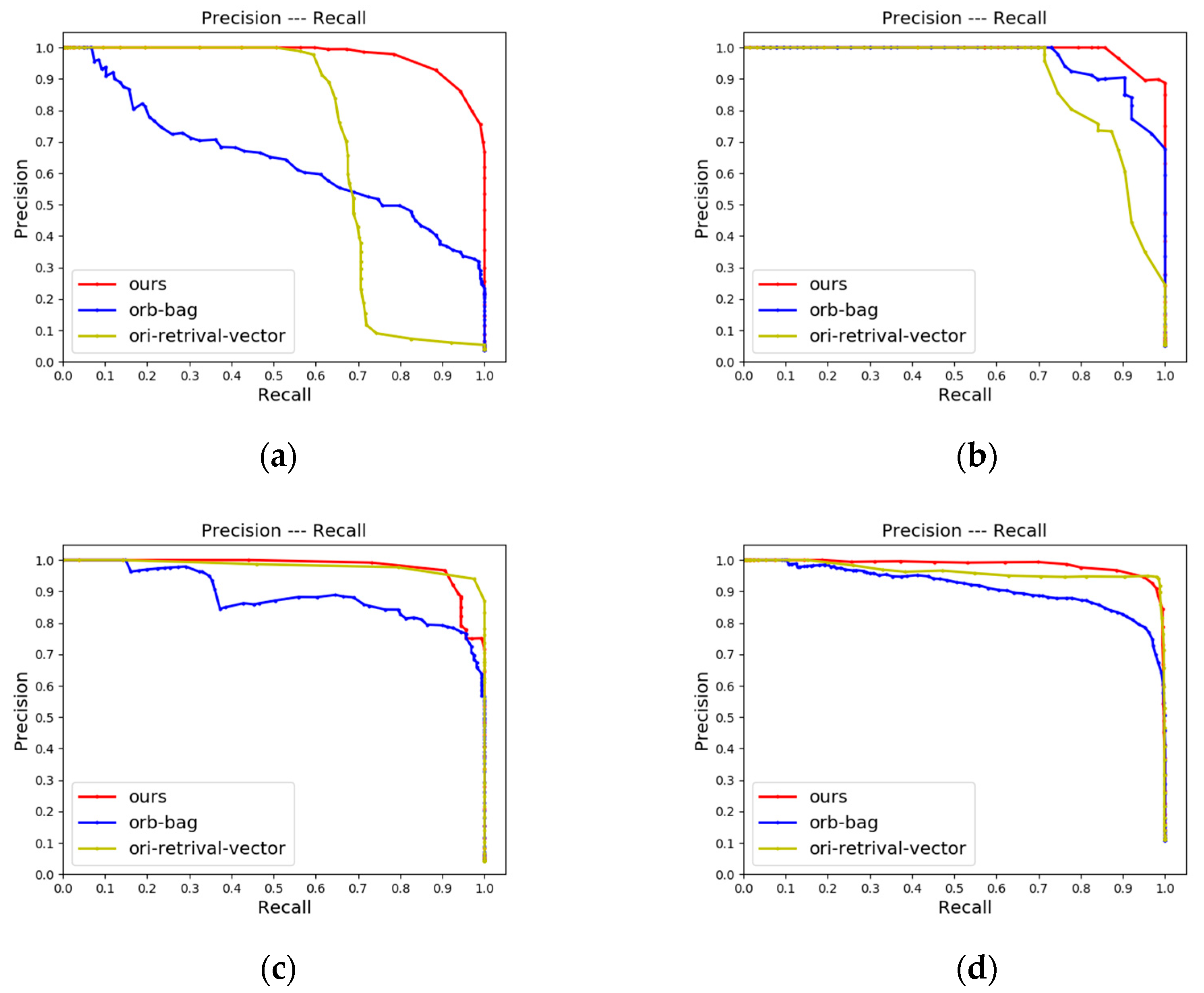
4.2.1. LCD Performance

The precision rate versus recall rate (P-R) curve and F1-score are adopted to compare the performances of the five algorithms. The F1-score is defined as:

$$F_1=2\times \frac{P\times R}{P+R}$$

(18)

where $P$ is the precision rate; $R$ is the recall rate; $F_1$ is the harmonic average of $P$ and $R$ of the model, which gives simultaneous consideration to the model’s precision rate and recall rate. Distinct loop acceptance thresholds are set within the interval [0, 1] in the experiments, and the P-R curves of the algorithms are plotted to evaluate the LCD performance.

First, our method is evaluated over the KITTI odometry sequences, using the original point cloud as the input to evaluate the performance of CMCD according to the P-R curves in Figure 6. It is found that ESF exhibits inferior performance on all datasets because this method relies on the histogram and cannot make an accurate distinction between positions unless the environmental change is great. M2DP delivers a very high precision rate at a very low recall rate on most of the datasets since it has correctly detected the obverse loop closure. However, without considering the rotational and translational changes of scenes, this method fails to detect the reverse loop closure, and the slopes of curves decrease rapidly. SC and ISC deliver relatively good detection performance, but neither possesses the rotation invariance in theory; they are implemented relying on brute-force matching, and both rely on vertical structural information, so their performance is limited when the vertical height in the environment varies little. Our method mainly relies on the projection approach to solve the translation transformation problem and on DTORB features to address contra-revisit. The detection performance of our method over both KITTI-00 and KITTI-05 is superior to all other methods and is almost on par with the best-performing SC over KITTI-02 and KITTI-06. Over the four sequences, the P-R curves of our method show a slight decrease in precision rate with the increase in recall rate, and the precision rate is still high at the maximum recall rate. The high recall rate signifies our method can effectively search the loop candidates with the less missing report, whereas the high precision rate can prevent erroneous loops from being registered into the map. According to Figure 6, the detection performances of all algorithms over KITTI-02 are poorer than over any other sequence, probably because the reverse loop closure in the data has the occlusion issue.

The experimental evaluation method over JLU datasets is the same as over KITTI odometry sequences. Through analysis of the performance of CMCD according to the P-R curves in Figure 7, it can be found that the overall performance is consistent with that of the KITTI odometry sequences. Since our datasets have been acquired by the 32-beam LiDAR, while the KITTI odometry sequences have been acquired by the 64-beam LiDAR, it is feasible to adopt DTORB of image features to decide whether a loop is constituted after projecting 3D point clouds into a 2D image. This approach is not only independent of LiDAR type, but it also has low equipment requirements, excellent robustness, and generalization ability. It can be found from Figure 7 that the LCD performances of M2DP and ESF remain inferior, and their effects are much unsatisfactory, especially over the dataset jlu00. Since the dataset jlu00 contains one segment of reverse loop closure, while neither M2DP nor ESF can recognize a reverse loop closure, the performance degrades dramatically. Point cloud occlusion is not severe in the relatively simple campus environment, so our algorithm can achieve a high precision rate over jlu00. Our algorithm delivers a higher precision rate than all the others at the same recall rate over the datasets jlu02 and jlu03. With the increase in recall rate, the precision rate of our scheme declines slowly, meaning that the LCD performance is stable. Additionally, among these sequences, the P-R curve of our algorithm almost completely covers those of other algorithms. Besides, the area under the curve of our algorithm is significantly larger than that of any other algorithm, demonstrating that our algorithm has outstanding discriminative performance and the ability to detect loop closure effectively. The performances of all algorithms are almost on par with the dataset jlu01, mainly because the scenes of this dataset only encompass a single segment of a positively directed loop.

4.2.2. Place Recognition Performance

EP score is used to evaluate the performance of our algorithm in place recognition. EP is defined as:

$$EP=\frac{1}{2} \left(P_{R0}+R_{P100}\right)$$

(19)

where $P_{R0}$ is the precision rate at the minimum recall rate; $R_{P100}$ is the maximum recall rate at 100% precision rate. $EP$ is an indicator specially used to evaluate the performance of a place recognition algorithm. See

Table 1. F1 scores and EP scores over KITTI odometry sequences and JLU datasets.

Methods	KITTI-00	KITTI-02	KITTI-05	KITTI-06	jlu00	jlu01	jlu02	jlu03
SC	0.9493/0.8719	0.8776/0.8746	0.9189/0.8326	0.9809/0.8957	0.8520/0.7407	0.9545/0.8809	0.8843/0.6776	0.9366/0.5396
ISC	0.8693/0.7141	0.8365/0.7935	0.8825/0.7564	0.9298/0.8677	0.8397/0.6485	0.9104/0.7857	0.8532/0.6056	0.8596/0.5321
M2DP	0.9188/0.7809	0.7902/0.5722	0.8892/0.5844	0.9328/0.6737	0.6667/0.4333	0.9185/0.7286	0.7717/0.3692	0.8970/0.4833
ESF	0.5653/0.4821	0.5589/0.4375	0.4795/0.2273	0.6216/0.45	0.1500/0.25	0.7285/0.53	0.4781/0.3226	0.5108/0.25
Ours	0.9754/0.8969	0.8950/0.8560	0.9729/0.8989	0.9827/0.9001	0.9056/0.7986	0.9403/0.8786	0.9359/0.7205	0.9478/0.5933

Notes: F1-score/EP score; figures in bold indicates the optimal performance.

for the comparison of EP score lists among different algorithms.

The F1 score is used to evaluate the robustness of LCD, and the EP score is used to evaluate the robustness of place recognition. From Table 1, the indicators of our method surpass other methods in most of the sequences. Over the dataset jlu00, where there exist two segments of obverse loop closure and one segment of reverse loop closure, the F1-score of our method is 0.9056, higher than that of the SC algorithm by 6%; the EP score of our algorithm is 0.7986, higher than that of the best-performing SC algorithm by 8%. This indicates our algorithm can accurately recognize obverse and reverse loop closures with higher robustness to rotational variation. The EP scores over most of the KITTI odometry sequences are all higher than those of other algorithms, meaning our algorithm can be used in preliminary place recognition. Over our own datasets, the LCD task is more challenging given the dynamic campus environment with a large number of pedestrians and parked vehicles. Although the EP score over the dataset jlu01 is slightly lower than that of the SC algorithm, the EP scores of our algorithm over other datasets are superior to other algorithms. For example, the EP score of our algorithm over the dataset jlu02 increases by 95% as compared to that of M2DP. Therefore, our method has good generalization ability and practical application value.

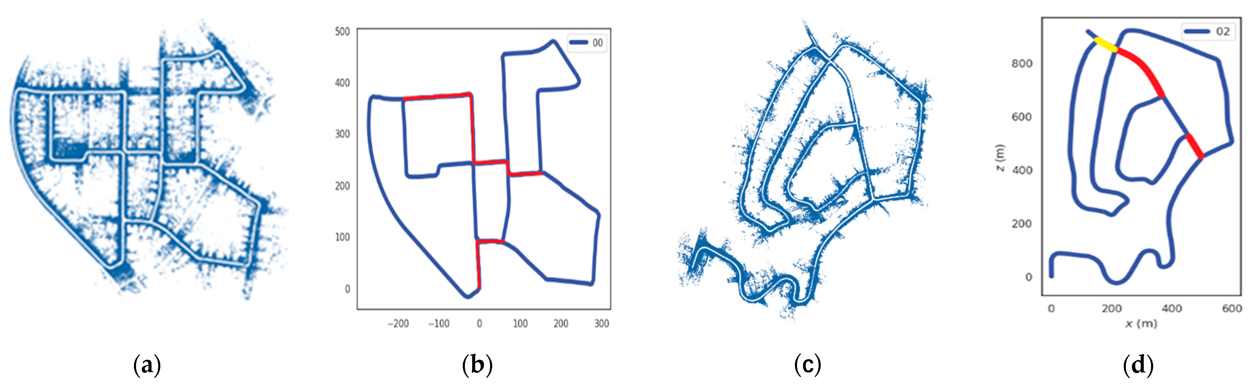
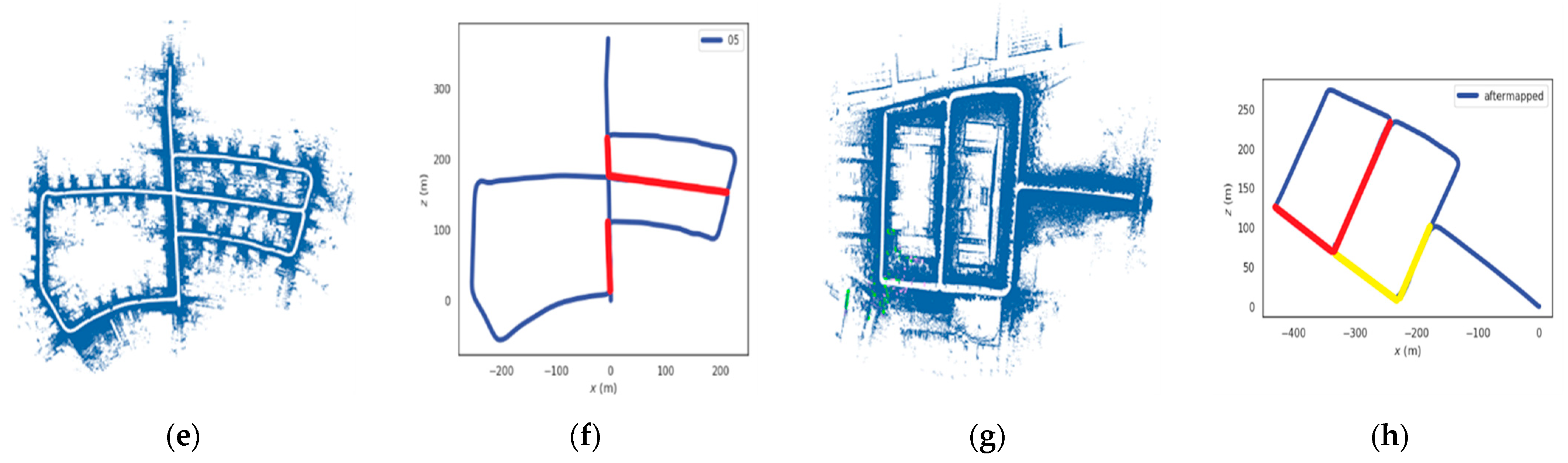
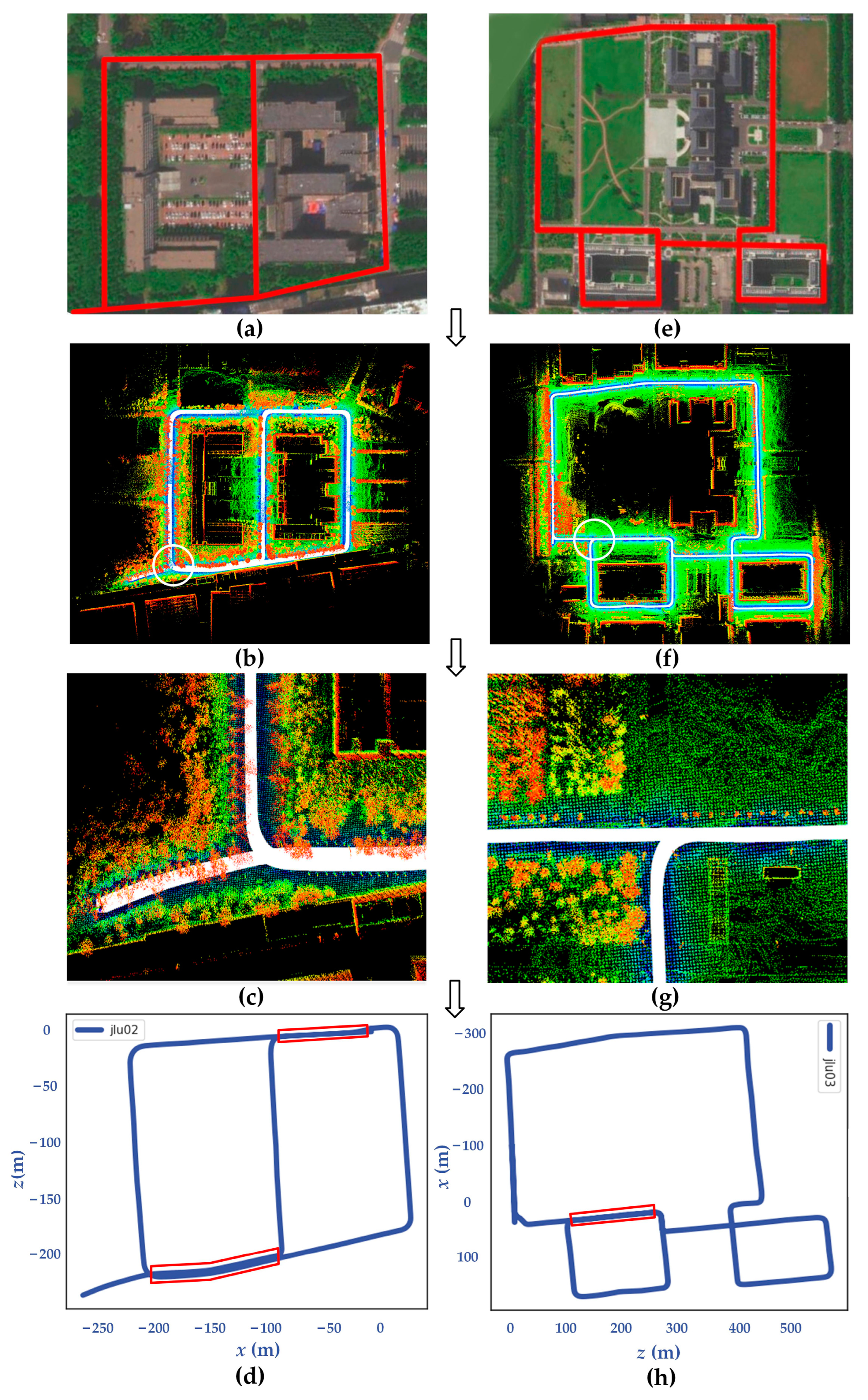
4.2.3. Improvement of the Mapping

In this experiment, the LCD module is added into the LeGO-LOAM [3,5,40] framework, using ICP [41] to match the current point clouds with historical ones of loop closure upon detecting loop closure, and a constraint factor is built. Afterward, the LiDAR odometry factor obtained at the frontend of LeGO-LOAM and the constraint factor obtained in our LCD scheme are both added into GTSAM [42] for mapping after backend optimization. The estimated trajectory on KITTI odometry sequences and JLU datasets after adding our own loop constraint into Lego-LOAM is shown in Figure 8. In Figure 8, the detected obverse loop closures are marked with red lines, and the detected reverse loop closure are marked with yellow lines. As shown in Figure 8a,b, the loop closures detected on the KITTI-00 sequence are completely closed in the map; the estimated trajectories show no intersection, overlap, or disconnection. As shown in Figure 8g,h, loop closures can still be accurately detected on the jlu00 sequence, thereby avoiding map drift. This suggests our method can accurately detect loop closure at different locations, avoid drift due to cumulative error, and improve the performance of mapping results. At the closed-loop position, the current trajectory coincides with the historical trajectory without ghosting and drift problems. In addition, wrong loop closure information is not registered in the estimated trajectory, so the accuracy of mapping is high. In addition, we show the mapping of jlu02 and jlu03 in detail. As can be seen from Figure 9, the constructed maps in jlu02 and jlu03 have no drift and ghost, where the overall layout of buildings and the extension direction of roads correspond to the scenes in Figure 9a,e. Figure 9b,c,f,g show the global mapping and local LCD results, respectively. Figure 9c,g is a magnification of the positions circled in Figure 9b,f, all of which are located in the closed part of the loop marked in red in Figure 9d,h. Therefore, the SLAM algorithm with CMCD as an LCD module can accurately detect loop closure in real scenes without errors.

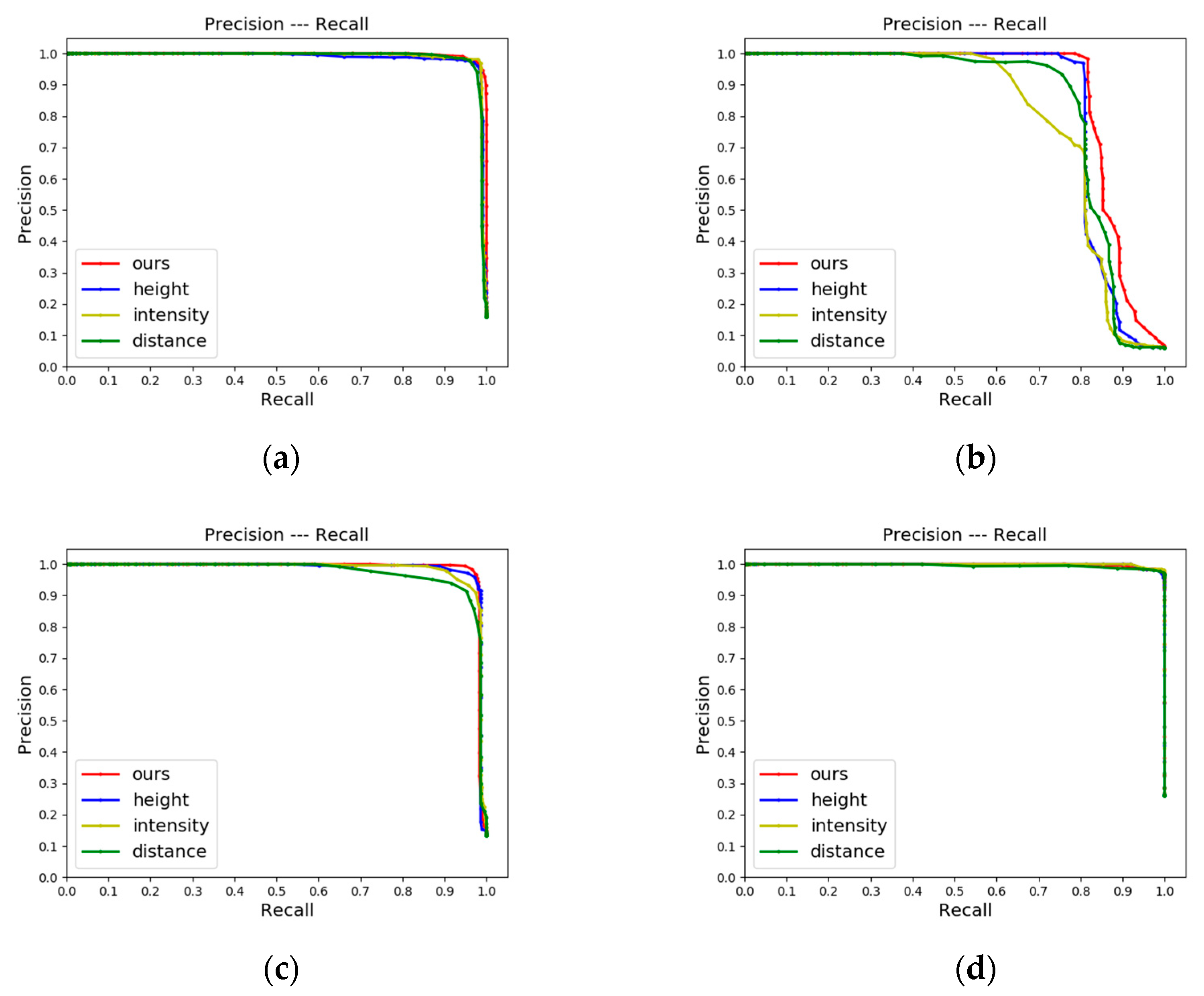
4.2.4. Ablation Experiments

In this section, we designed three groups of ablation experiments to analyze the impact of three methods, namely different point cloud projections, different similarity measurements, and retrieval vectors with or without enhancement, on loop closure detection performance.

In the first ablation experiment, we compare the performance of four projection methods, CMCD, bird-eye view projection using height information, bird-eye view projection using intensity information, and bird-eye view projection using distance information, on the KITTI odometry sequences and JLU datasets. The main difference between these four methods is different projection strategies, and other experimental settings are unchanged. Figure 10 shows the CMCD projection of a frame point cloud in KITTI odometry sequences and JLU datasets, respectively as well as the simple bird’s eye view of height, intensity, and distance. As can be seen from Figure 10, the three simple projections are different in detail, which indicates that the information they provide will be different. This further indicates that more feature information can be obtained by combining them to improve the performance of the algorithm.

The P-R curves in Figure 11 and Figure 12 show the difference in algorithm performance between the four projection methods due to different feature information. According to the experimental results, we can find that firstly, CMCD improves in both accuracy and recall of loop closure detection with a larger area under the curve compared to projection using a single message. Secondly, CMCD seems to be more accurate on sequences with reverse loop closure (refer to the results of sequences KITTI-02, jlu00 in Figure 11 and Figure 12). One possible explanation is that the global descriptor information is richer and more discriminative due to the multi-channel encoding, which reduces the occurrence of false matches. Finally, this experiment can find that CMCD detects loop closure significantly better than other schemes on the JLU datasets (refer to the results of sequences jlu00 and jlu03 in Figure 12). The JLU datasets are collected by 32-beam LiDAR, and the number of point clouds in a single frame is not as rich as 64-beam LiDAR used by KITTI odometry sequences. Thus, the information loss is more serious after using single-channel projection, which leads to poor loop closure detection performance. It can be concluded that our CMCD method can significantly improve the information content and lead to better performance.

In the second ablation experiment, we compared our method with the method using the bag-of-words model constructed by DTORB features for retrieval on KITTI odometry sequences and JLU datasets, respectively. The main difference between them is the different strategies of similarity metrics. The red and blue lines in Figure 13 and Figure 14 are the results of our method and the bag-of-words model method, respectively. It can be seen from the figures that in most scenarios on KITTI odometry sequences and JLU datasets, the P-R curve (red lines) of the proposed method is above the compared method (blue lines). This indicates that the retrieval effect of our method is better than the compared method in most cases. Our result is slightly worse than the compared method on KITTI-02. The main reason is that the trajectory of KITTI-02 is more complex than the other three sequences containing loops. It makes the scene vary greatly, and the discrimination between word vectors is better. This indicates that the retrieval strategy based on the bag-of-words model depends on the richness of features and the size of the bag of words. Because the dictionary needs to be built in advance, its effect and stability are difficult to predict in advance.

In the third ablation experiment, we used two different retrieval vectors. One is the enhanced retrieval vector proposed in this paper, and the other is the ordinary retrieval vector (ori-retrieval-vector). The ordinary retrieval vector is obtained by taking the L1-norms of all rows for the descriptor and summing them. Other experimental settings are unchanged. An illustration of the selected candidates is shown in Figure 15. According to the enhanced retrieval vector, we find the ten most similar loop candidates of frame 2582 of KITTI-05 and frame 3715 of jlu02, respectively. The frame IDs of the ten most similar loop candidates of frame 2582 are 145, 819, 820, 822, 823, 834, 835, 836, 887, and 1998 respectively. The frame IDs of the ten most similar loop candidates of frame 3715 are 1314, 1318, 2841, 2842, 2843, 2847, 2848, 2849, 2850, and 2851, respectively.

The loop closure detection results of two retrieval vectors on different data sets are located in Figure 13 and Figure 14. By comparing the red line (enhanced retrieval vector proposed in this paper) and the yellow line (original retrieval vector) in Figure 13 and Figure 14, it can be seen that the enhanced retrieval vector has a more significant effect. The area wrapped by the P-R curve is obviously larger on the data with longer distances and more frames, such as KITTI-00, KITTI-02, KITTI-05, jlu00, and jlu01. The visualization shows that our algorithm can not only find the most similar frame but also find the region where the loop is located, indicating that our algorithm has good robustness.

4.2.5. Analysis of Computation Time

To evaluate the real-time performance and computational complexity of the proposed method, we adopt the following two methods for analysis: (1) Analyze the time complexity of the proposed method, which is O$(M\times N+K$). $M$ and $N$ are the length and width of the image, and $K$ is the number of point cloud frames. (2) Calculate the average execution time of each frame point cloud. Specifically, we calculate and accumulate the processing time of each frame point cloud from the initial projection process to the final selection of the most similar candidate frames. Furthermore, we divide the total processing time above by the total frames to obtain the average execution time.

Table 2. Average execution time over KITTI odometry sequences and JLU datasets.

Methods	Avg KITTI Execution Time (s/Query)				Avg JLU Execution Time (s/Query)
	KITTI-00	KITTI-02	KITTI-05	KITTI-06	jlu00	jlu01	jlu02	jlu03
SC	0.0867	0.0861	0.0885	0.0846	0.0583	0.0558	0.0658	0.0732
ISC	0.0697	0.0687	0.0678	0.0656	0.0537	0.0513	0.0580	0.0605
M2DP	0.3655	0.3873	0.3869	0.3827	0.3974	0.3554	0.3739	0.3538
ESF	0.0728	0.0784	0.0785	0.0664	0.0724	0.0574	0.0541	0.0655
Ours	0.0603	0. 0601	0.0589	0.0525	0.0587	0.0483	0.0539	0.0598

Notes: figures in bold indicates the optimal performance.

shows the average execution time per frame of the point cloud for different methods.

As can be seen, the average execution time of each frame of our method is lower than that of other method on the KITTI odometry sequences. As for JLU datasets, the average execution time for each frame of our algorithm in jlu01, jlu02, and jlu03 is lower than that of other methods. Although the execution time in jlu01 is slightly poor, it is also within the acceptable range. In the future, we will continue to improve the DTORB features to optimize the execution time of the algorithm.

5. Conclusions

In this paper, we have proposed a novel method for the construction of global descriptors, CMCD. Multi-channel descriptors have been constructed by the CMCD method; then, DTORB features have been extracted for the descriptors; finally, the similarity score between point clouds has been calculated according to the features. Overall, our algorithm has made full use of the structural information of point clouds and compressed the point cloud information into a 2D image, thereby introducing the visual method into the LiDAR point clouds. Compared with the state-of-the-art LCD methods, our method has achieved an average precision rate of 0.9565 and an average recall rate of 0.8879 over the KITTI odometry sequences, and a maximum precision rate of 0.9478 and a maximum recall rate of 0.8786 over our own datasets. The experiments have demonstrated that our algorithm can accurately detect loop closure with high efficiency and robustness. We plan to extend our method to point cloud matching and try to apply more mature and efficient visual SLAM methods to the LiDAR algorithm in the future.

References

1. Huang, B.; Zhao, J.; Liu, J. A Survey of Simultaneous Localization and Mapping. arXiv 2019, arXiv:1909.05214. [Google Scholar]
2. Zhang, J.; Singh, S. LOAM: Lidar odometry and mapping in real-time. In Proceedings of the Robotics: Science and Systems, Berkeley, CA, USA, 12–16 July 2014; pp. 1–9. [Google Scholar]
3. Shan, T.; Englot, B. Lego-loam: Lightweight and ground-optimized lidar odometry and mapping on variable terrain. In Proceedings of the 2018 IEEE/RSJ International Conference on Intelligent Robots and Systems (IROS), Madrid, Spain, 1–5 October 2018; pp. 4758–4765. [Google Scholar]
4. Shan, T.; Englot, B.; Meyers, D.; Wang, W.; Ratti, C.; Rus, D. Lio-sam: Tightly-coupled lidar inertial odometry via smoothing and mapping. In Proceedings of the 2020 IEEE/RSJ International Conference on Intelligent Robots and Systems (IROS), Las Vegas, NV, USA, 25–29 October 2020; pp. 5135–5142. [Google Scholar]
5. Chen, S.; Zhou, B.; Jiang, C.; Xue, W.; Li, Q. A LiDAR/Visual SLAM Backend with Loop Closure Detection and Graph Optimization. Remote Sens. 2021, 13, 2720. [Google Scholar] [CrossRef]
6. Wang, W.; Liu, J.; Wang, C.; Luo, B.; Zhang, C. DV-LOAM: Direct visual lidar odometry and mapping. Remote Sens. 2021, 13, 3340. [Google Scholar] [CrossRef]
7. Rublee, E.; Rabaud, V.; Konolige, K.; Bradski, G. ORB: An efficient alternative to SIFT or SURF. In Proceedings of the 2011 International Conference on Computer Vision, Barcelona, Spain, 6–13 November 2011; pp. 2564–2571. [Google Scholar]
8. Mur-Artal, R.; Montiel, J.M.M.; Tardos, J.D. ORB-SLAM: A versatile and accurate monocular SLAM system. IEEE Trans. Robot. 2015, 31, 1147–1163. [Google Scholar] [CrossRef] [Green Version]
9. Derpanis, K.G. Overview of the RANSAC Algorithm. Image Rochester NY 2010, 4, 2–3. [Google Scholar]
10. Kim, G.; Kim, A. Scan context: Egocentric spatial descriptor for place recognition within 3d point cloud map. In Proceedings of the 2018 IEEE/RSJ International Conference on Intelligent Robots and Systems (IROS), Madrid, Spain, 1–5 October 2018; pp. 4802–4809. [Google Scholar]
11. Kim, G.; Choi, S.; Kim, A. Scan context++: Structural place recognition robust to rotation and lateral variations in urban environments. IEEE Trans. Robot. 2021, 38, 1856–1874. [Google Scholar] [CrossRef]
12. Shan, T.; Englot, B.; Duarte, F.; Ratti, C.; Rus, D. Robust place recognition using an imaging lidar. In Proceedings of the 2021 IEEE International Conference on Robotics and Automation (ICRA), Xi’an, China, 30 May–5 June 2021; pp. 5469–5475. [Google Scholar]
13. Sivic, J.; Zisserman, A. Video Google: A text retrieval approach to object matching in videos. In Proceedings of the IEEE International Conference on Computer Vision, Nice, France, 13–16 October 2003; pp. 1470–1477. [Google Scholar]
14. Cummins, M.; Newman, P. FAB-MAP: Probabilistic localization and mapping in the space of appearance. Int. J. Robot. Res. 2008, 27, 647–665. [Google Scholar] [CrossRef]
15. Bay, H.; Tuytelaars, T.; Gool, L.V. Surf: Speeded up robust features. In Proceedings of the European Conference on Computer Vision, Graz, Austria, 7–13 May 2006; pp. 404–417. [Google Scholar]
16. Mur-Artal, R.; Tardós, J.D. Fast relocalisation and loop closing in keyframe-based SLAM. In Proceedings of the 2014 IEEE International Conference on Robotics and Automation (ICRA), Hong Kong, China, 31 May–7 June 2014; pp. 846–853. [Google Scholar]
17. Gálvez-López, D.; Tardos, J.D. Bags of binary words for fast place recognition in image sequences. IEEE Trans. Robot. 2012, 28, 1188–1197. [Google Scholar] [CrossRef]
18. Wohlkinger, W.; Vincze, M. Ensemble of shape functions for 3d object classification. In Proceedings of the 2011 IEEE International Conference on Robotics and Biomimetics, Karon Beach, Thailand, 7–11 December 2011; pp. 2987–2992. [Google Scholar]
19. Rusu, R.B.; Blodow, N.; Beetz, M. Fast point feature histograms (FPFH) for 3D registration. In Proceedings of the 2009 IEEE International Conference on Robotics and Automation, Kobe, Japan, 12–17 May 2009; pp. 3212–3217. [Google Scholar]
20. Bosse, M.; Zlot, R.; Flick, P. Zebedee: Design of a spring-mounted 3-d range sensor with application to mobile mapping. IEEE Trans. Robot. 2012, 28, 1104–1119. [Google Scholar] [CrossRef]
21. Dubé, R.; Dugas, D.; Stumm, E.; Nieto, J.; Siegwart, R.; Cadena, C. Segmatch: Segment based place recognition in 3d point clouds. In Proceedings of the 2017 IEEE International Conference on Robotics and Automation (ICRA), Singapore, 29 May–3 June 2017; pp. 5266–5272. [Google Scholar]
22. Uy, M.A.; Lee, G.H. Pointnetvlad: Deep point cloud based retrieval for large-scale place recognition. In Proceedings of the IEEE Conference on Computer Vision and Pattern Recognition, Salt Lake City, UT, USA, 18–22 June 2018; pp. 4470–4479. [Google Scholar]
23. Qi, C.R.; Su, H.; Mo, K.; Guibas, L.J. Pointnet: Deep learning on point sets for 3d classification and segmentation. In Proceedings of the IEEE Conference on Computer Vision and Pattern Recognition, Honolulu, HI, USA, 21–26 July 2017; pp. 652–660. [Google Scholar]
24. Arandjelovic, R.; Gronat, P.; Torii, A.; Pajdla, T.; Sivic, J. NetVLAD: CNN architecture for weakly supervised place recognition. In Proceedings of the IEEE Conference on Computer Vision and Pattern Recognition, Las Vegas, NV, USA, 27–30 June 2016; pp. 5297–5307. [Google Scholar]
25. He, L.; Wang, X.; Zhang, H. M2DP: A novel 3D point cloud descriptor and its application in loop closure detection. In Proceedings of the 2016 IEEE/RSJ International Conference on Intelligent Robots and Systems (IROS), Daejeon, Korea, 9–14 October 2016; pp. 231–237. [Google Scholar]
26. Wang, H.; Wang, C.; Xie, L. Intensity scan context: Coding intensity and geometry relations for loop closure detection. In Proceedings of the 2020 IEEE International Conference on Robotics and Automation (ICRA), Paris, France, 31 May–31 August 2020; pp. 2095–2101. [Google Scholar]
27. Wang, Y.; Sun, Z.; Xu, C.-Z.; Sarma, S.E.; Yang, J.; Kong, H. Lidar iris for loop-closure detection. In Proceedings of the 2020 IEEE/RSJ International Conference on Intelligent Robots and Systems (IROS), Las Vegas, NV, USA, 25–29 October 2020; pp. 5769–5775. [Google Scholar]
28. Luo, L.; Cao, S.-Y.; Han, B.; Shen, H.-L.; Li, J. BVMatch: Lidar-Based Place Recognition Using Bird’s-Eye View Images. IEEE Robot. Autom. Lett. 2021, 6, 6076–6083. [Google Scholar] [CrossRef]
29. Chen, X.; Läbe, T.; Milioto, A.; Röhling, T.; Vysotska, O.; Haag, A.; Behley, J.; Stachniss, C. OverlapNet: Loop closing for LiDAR-based SLAM. arXiv 2021, arXiv:2105.11344. [Google Scholar]
30. Hou, W.; Li, D.; Xu, C.; Zhang, H.; Li, T. An advanced k nearest neighbor classification algorithm based on KD-tree. In Proceedings of the 2018 IEEE International Conference of Safety Produce Informatization (IICSPI), Chongqing, China, 10–12 December 2018; pp. 902–905. [Google Scholar]
31. Shlens, J. A tutorial on principal component analysis. arXiv 2014, arXiv:1404.1100. [Google Scholar]
32. Rosten, E.; Drummond, T. Machine learning for high-speed corner detection. In Proceedings of the European Conference on Computer Vision, Graz, Austria, 7–13 May 2006; pp. 430–443. [Google Scholar]
33. Calonder, M.; Lepetit, V.; Strecha, C.; Fua, P. Brief: Binary robust independent elementary features. In Proceedings of the European Conference on Computer Vision, Crete, Greece, 5–11 September 2010; pp. 778–792. [Google Scholar]
34. Meer, P.; Mintz, D.; Rosenfeld, A.; Kim, D.Y. Robust regression methods for computer vision: A review. Int. J. Comput. Vis. 1991, 6, 59–70. [Google Scholar] [CrossRef]
35. The Code of SC Algorithm. Available online: https://github.com/gisbi-kim/scancontext (accessed on 24 September 2021).
36. The Code of ISC Algorithm. Available online: https://github.com/wh200720041/iscloam (accessed on 13 March 2021).
37. The Code of M2DP Algorithm. Available online: https://github.com/gloryhry/M2DP-CPP (accessed on 14 January 2022).
38. The Code of ESF Algorithm. Available online: http://pointclouds.org/documentation/classpcl_1_1_e_s_f_estimation.html (accessed on 15 November 2021).
39. Geiger, A.; Lenz, P.; Stiller, C.; Urtasun, R. Vision meets robotics: The kitti dataset. Int. J. Robot. Res. 2013, 32, 1231–1237. [Google Scholar] [CrossRef]
40. Xue, G.; Wei, J.; Li, R.; Cheng, J. LeGO-LOAM-SC: An Improved Simultaneous Localization and Mapping Method Fusing LeGO-LOAM and Scan Context for Underground Coalmine. Sensors 2022, 22, 520. [Google Scholar] [CrossRef] [PubMed]
41. Rusinkiewicz, S.; Levoy, M. Efficient variants of the ICP algorithm. In Proceedings of the Third International Conference on 3-D Digital Imaging and Modeling, Quebec City, QC, Canada, 28 May–1 June 2001; pp. 145–152. [Google Scholar]
42. Dellaert, F. Factor Graphs and GTSAM: A Hands-On Introduction; Georgia Institute of Technology: Atlanta, GA, USA, 2012. [Google Scholar]
Figure 1. Schematic of CMCD blocks for multi-channel descriptors. The red area represents a pixel in the figure, and the point cloud in the corresponding three-dimensional region of the red area will be projected into this pixel.
Remotesensing 14 05877 g001
Figure 2. System overview.
Remotesensing 14 05877 g002
Figure 3. A visual illustration of the CMCD coding process: each channel corresponds to distance, intensity, and height information, respectively.
Remotesensing 14 05877 g003
Figure 4. The execution result figure of selection of loop candidate: retrieve the ten most similar loop candidates of the point cloud at frame 2582 of KITTI-05.
Remotesensing 14 05877 g004
Figure 5. The visualization of DTORB matching progress, they should be listed as (a,b) two pairs of LCD in KITTI-05; (c,d) the visualization of matching performed by traditional ORB; (e,f) the visualization of the proposed DTORB.
Remotesensing 14 05877 g005aRemotesensing 14 05877 g005b
Figure 6. P-R curves corresponding to KITTI odometry sequences should be listed as the (a) P-R curve of KITTI-00; (b) P-R curve of KITTI-02; (c) P-R curve of KITTI-05; (d) P-R curve of KITTI-06.
Remotesensing 14 05877 g006
Figure 7. P-R curves corresponding to JLU datasets should be listed as the (a) P-R curve of jlu00; (b) P-R curve of jlu01; (c) P-R curve of jlu02; (d) P-R curve of jlu03.
Remotesensing 14 05877 g007
Figure 8. Mapping and LCD results should be listed as the (af) mapping and LCD results on KITTI-00, KITTI-02, and KITTI-05; (g,h) mapping and LCD results on jlu00. The red and yellow lines indicate the detected obverse and reverse loop closures, respectively.
Remotesensing 14 05877 g008aRemotesensing 14 05877 g008b
Figure 9. The mapping results of CMCD in SLAM on jlu02 and 03: (a,e) BEV images of jlu02 and jlu05, the red lines represent the driving route at the time of data collection; (b,f) the visualized results of the point cloud map; (c,g) the local LCD results; (d,h) the mapping and LCD results, the red box indicates that this trajectory has loop closure.
Remotesensing 14 05877 g009
Figure 10. Illustration of CMCD and simple bird’s eye view projection: (a) The CMCD projection of frame 2582 on KITTI-05 (as shown in (4)) and the corresponding single-channel projection of height, intensity, and distance (as shown in (1), (2) and (3), respectively); (b) The CMCD projection of frame 3715 of jlu02 (as shown in (5)) and the corresponding single-channel projection of height, intensity, and distance (as shown in (6), (7) and (8), respectively). In the legend, “Height: 1; Intensity: 0; Distance: 0,” indicates that the image is projected according to the height information.
Remotesensing 14 05877 g010
Figure 11. P-R curves of CMCD, single-channel projection of height, intensity, and distance on KITTI Odometry sequences: (a) The P-R curve of KITTI-00; (b) The P-R curve of KITTI-02; (c) The P-R curve of KITTI-05; (d) The P-R curve of KITTI-06.
Remotesensing 14 05877 g011
Figure 12. P-R curves of CMCD, single-channel projection of height, intensity, and distance on JLU datasets: (a) P-R curve of jlu00; (b) P-R curve of jlu01; (c) P-R curve of jlu02; (d) P-R curve of jlu03.
Remotesensing 14 05877 g012
Figure 13. P-R curves of CMCD, orb-bag, and ori-retrieval-vector on KITTI odometry sequences: (a) The P-R curve of KITTI-00; (b) The P-R curve of KITTI-02; (c) The P-R curve of KITTI-05; (d) The P-R curve of KITTI-06.
Remotesensing 14 05877 g013
Figure 14. P-R curves of CMCD, orb-bag, and ori-retrieval-vector on JLU datasets: (a) The P-R curve of jlu00; (b) The P-R curve of jlu01; (c) The P-R curve of jlu02; (d) The P-R curve of jlu03.
Remotesensing 14 05877 g014
Figure 15. The retrieval results of the enhanced retrieval vector: (a) frame 2582 of KITTI-05 and its candidate set; (b) frame 3715 of jlu02 and its candidate set.
Remotesensing 14 05877 g015