Abstract
The monitoring of ships is of paramount importance for ocean and coastal area surveillance. The synthetic aperture radar is shown to be a key sensor to provide effective and continuous observation of ships due to its unique imaging capabilities. When advanced synthetic aperture radar imaging systems are considered, the full scattering information is available that was demonstrated to be beneficial in developing improved ship detection and classification algorithms. Nonetheless, the capability of polarimetric synthetic aperture radar to observe marine vessels is significantly affected by several imaging and environmental parameters, including the incidence angle. Nonetheless, how changes in the incidence angle affect the scattering of ships still needs to be further investigated since only a sparse analysis, i.e., on different kinds of ships of different sizes observed at multiple incidence angles, has been performed. Hence, in this study, for the first time, the polarimetric scattering of the same ship, i.e., a small fishing trawler, which is imaged multiple times under the same sea state conditions but in a wide range of incidence angles, is analysed. This unique opportunity is provided by a premium L-band UAVSAR airborne dataset that consists of five full-polarimetric synthetic aperture radar scenes collected in the Gulf of Mexico. Experimental results highlight the key role played by the incidence angle on both coherent, i.e., co-polarisation signature and pedestal height, and incoherent, i.e., multi-polarisation and total backscattering power, polarimetric scattering descriptors. Experimental results show that: (1) the polarised scattering component is more sensitive to the incidence angle with respect to the unpolarised one; (2) the co-polarised channel under horizontal polarisation dominated the polarimetric backscattering from the fishing trawler at lower angles of incidence, while both co-polarised channels contribute to the polarimetric backscattering at higher incidence angles; (3) the HV polarisation provides the largest target-to-clutter ratio at lower incidence angles, while the HH polarisation should be preferred at higher angles of incidence.
1. Introduction
The synthetic aperture radar (SAR) is a microwave remote sensing tool that, due to its all-day and almost all-weather imaging capabilities together with its fine spatial resolution and wide area coverage, is a key instrument for open ocean and coastal area surveillance, including the observation of metallic targets at sea [1,2]. SAR monitoring of marine vessels is an important application that triggered the development of many approaches that can be roughly classified in image processing- and scattering-based methods. When dealing with the latter, several methods, which are either based on single- [3,4] or multi-polarisation measurements [5,6,7], have been proposed. Generally speaking, SAR observation of ships relies on the fact that the metallic structures of marine vessels are characterised by a backscattered signal stronger than the one from the surrounding sea. However, the difference in sea–ship backscattering is severely affected by SAR imaging parameters, e.g., incident wavelength and incidence angle, meteo-marine conditions and by the properties of the marine vessel, e.g., the material it consists of, the heading, and the geometric structure. This effect, together with the availability of more advanced Earth observation satellite missions equipped with polarimetric SAR (polSAR) imaging sensors, triggered the development of scattering-based marine vessel observation approaches. Hence, for the purpose of this study, a brief overview of polSAR methods to monitor marine vessels is due.
In [8], a constant false alarm rate (CFAR) method was proposed to detect ships—according to the polarimetric whitening filter detector—in simulated and actual C-band NASA (National Aeronautics and Space Administration)/JPL (Jet Propulsion Laboratory) AIRSAR (Airborne SAR) airborne polSAR imagery. The results demonstrate the importance of statistical modelling of sea clutter in developing CFAR methods and that the proposed detector outperforms the conventional two-parameter CFAR especially when a low target-to-clutter ratio (TCR) applies. In [9], a ship detection algorithm that combines the polarisation cross-entropy feature derived from the eigen-decomposition of the polSAR coherency matrix and a CFAR method was proposed. Experimental results, undertaken on C-band NASA/JPL AIRSAR airborne data show that the coherent information exploited by the proposed detector allows distinguishing ships from the background sea better than detectors based on incoherent information, i.e., the total backscattered power and the cross-polarised backscattering intensity. In [10], ships were observed using full-polarimetric L- and C-band imagery from the Advanced Land Observing Satellite (ALOS) Phased Array type L-band Synthetic Aperture Radar (PALSAR) and the Radarsat-2 polSAR satellite missions. Two detectors based on the different polarimetric scattering properties that characterise marine vessels and sea surface, i.e., reflection symmetry and level of scattering depolarisation, were proposed. Results demonstrate the effectiveness of using polarimetric scattering descriptors to enhance the observation of ships. In [11], the different speckle characteristics that affect ship and sea cross-polarised backscattering were exploited to effectively characterise marine vessels. Results obtained from C-band full-polarimetric Radarsat-2 SAR data show the key role played by the coherent scattering component in detecting the ships. In [12], a geometrical perturbation-polarimetric notch filter was developed to detect ships in polSAR imagery. Experimental results relevant to a X-band TerraSAR-X full-polarimetric SAR dataset demonstrate that the proposed approach is robust with respect to sea state conditions and that its detection performance depends on the ship’s size. In [13], C-band Gaofen-3 satellite SAR images and L-band UAVSAR (Uninhabited Aerial Vehicle SAR) and AIRSAR airborne polSAR measurements were considered to detect small ships by exploiting their polarimetric scattering behaviour. Results, based on the TCR metric, showed that surface scattering is the dominant scattering mechanism for most of the small ships and that this information is beneficial to enhance the detectability of small ships, especially when a rough sea surface is in place. In [14], since the detectability of ships in SAR imagery is significantly affected by the scattering process, the ship detection performance was discussed against the incident wavelength. C-band Sentinel-1 and X-band TerraSAR-X satellite SAR measurements were analysed and the TCR was considered as the figure of merit. They found that the X-band shorter wavelength results in a larger TCR if compared to the longer C-band wavelength. In [15], a scattering model-based approach was developed to detect ships in actual C-band full-polarimetric Radarsat-2 and SIR-C/X (Spaceborne Imaging Radar) SAR imagery as well as in simulated compact polarimetric SAR data. Experimental results demonstrate that the detection performance is sensitive to the transmitted polarisation and that the ellipticity angle, together with the relative phase of the two compact polarimetric channels, are effective in detecting marine vessels. Together with scattering-based ship detection algorithms, it must be pointed out that, in the recent years, advanced machine learning-based methods, including deep learning, have been proposed [16,17,18,19,20]. It was shown that they allow detecting ships in a very accurate, robust, and effective way, providing high detection probabilities and low false alarm rates under different SAR imaging parameters and environmental conditions.
A fundamental aspect that arises from the analysis of polSAR-based methods for ship monitoring is that polarimetric scattering of marine vessels depends significantly on SAR imaging parameters and environmental conditions. Among the former ones, the angle of incidence (AOI) plays a key role [21,22,23]. Nonetheless, in the literature, few studies addressed the effects of AOI on polSAR scattering of marine vessels and, in addition, those studies only refer to different ships, with different sizes, observed at sparse AOI. In [21], the sensitivity of multi-polarisation features to ships was investigated by means of full-polarimetric C-band polSAR measurements collected by an airborne platform. The performance of different detectors were investigated and ranked according to the TCR metric, which was discussed against AOI and polarisation. Experimental results show that the HH- and HV-polarised backscattering information results in the largest TCR for incidence angles > and <, respectively. In [22], a dataset that consists of forty-three ships of different sizes imaged by the airborne Convair-580 SAR system was used to discuss the TCR against the polarisation and AOI. Results suggest that the AOI remarkably impacts the TCR, whose largest values were obtained at HH and VV polarisation when high and low AOIs were considered, respectively. In [23], ten marine vessels of different size were observed using full-polarimetric Radarsat-2 SAR measurements collected under different sea state conditions at AOIs falling in the range 29–40. Both coherent and incoherent polSAR features were considered that were shown to be more effective than the single-polarisation backscattering intensities in detecting ships. They also observed that the cross-polarised backscattering intensity provides a TCR larger than that of the co-polarised ones at lower AOIs and that the degree of polarisation is almost AOI-independent.
The key issue that stems from the above discussion relies on the strong link between the scattering properties of marine vessels and the AOI. Although this issue has been addressed in the literature, there are still some uncertainties that mainly results from the use of multiple datasets where different ships are imaged at different AOIs and a lack of an in-depth analysis on the change in scattering characteristics when varying the AOI.
Hence, in this study, the polarimetric scattering of a small ship, i.e., a fishing trawler, is investigated in the L-band by means of a full-polarimetric UAVSAR dataset collected in a wide range of AOI (about 35–50). The study is performed under given conditions, i.e., the same low-to-moderate sea state conditions and true heading of the ship under analysis at the time of the UAVSAR flight. Accordingly, this premium high-quality dataset offered the unique opportunity of investigating the effects of AOI in the L-band polarimetric scattering of a small ship, which represents a challenging case study due to the small size of the target under investigation if compared with the spatial resolution of the SAR sensor. It is also worth noting that the analysis tools used in this study can be applied even to larger ships where, nonetheless, it is likely to expect that they are characterised by a very different structure. To the best of our knowledge, the multi-polarisation L-band scattering properties of a small ship observed under the same imaging conditions except for the incidence angle are analysed in this study for the first time. The findings presented in this study will help in better understanding the polarimetric scattering process and, since several ship detection and classification algorithms have been proposed that rely on the scattering features of the target extracted from polarimetric SAR imagery [8,12,13,21], to improve the performance of existing methods and foster the development of more advanced and robust techniques.
2. Theoretical Background
In this section, a brief polarimetric background is provided. A full-polarimetric SAR measures the scattering matrix that links the incident wave with the scattered one [24]:
where and are the scattered and incident electric fields, respectively, j is the imaginary unit, k is the wave number, r represents the distance between the SAR and the target and the subscripts H and V stand for horizontal and vertical polarisations, respectively. In (1), the scattering matrix is a complex-valued matrix whose elements are termed scattering amplitudes. The scattering amplitudes, for each combination of transmitting and receiving polarisation, represent the capability of the targets within the SAR resolution cell to scatter off the electromagnetic energy received from the sensor. It is worth noting that, once the acquisition geometry is given, they depend on the observed target only. When dealing with a random distributed targets, the Jones formalism (1) is not suitable and a more general formalism must be adopted which is based on the Stokes formalism [24]:
The Stokes vector associated with the wave scattered by the observed scene is related to the incident one through the Mueller matrix which is a non-symmetric real value matrix that, in the backscattering case, is given by [24,25,26]:
where ⊗ is the direct product between two matrices, means ensemble average, while the superscript * stands for complex conjugate. Equation (2) represents a second-order incoherent scattering model and it is the most general way to deal with polarimetric scattering. The Mueller matrix contains basic elements to synthesise the power measured from any combination of transmit/receive antenna polarisation basis. Under the backscatter alignment convention, the normalised radar cross section (NRCS) for a given transmitted (subscript q) and received (subscript p) polarisation is given by:
where stands for the NRCS, the superscript T means transpose, is a zero matrix whose diagonal elements are 1, 1, 1, and −1, and are the given transmitting and receiving antennas’ polarisation described according to the Stokes formalism:
where and are the ellipticity and orientation angle, respectively, defined in the polarisation plane, see Figure 1. The polarisation signature is typically displayed in the co- and cross-polarised cases, i.e., ; and + 90; + 90, respectively, using (4). The linear and circular polarisation can be achieved by varying the and angles. The linearly polarised waves can be achieved for any when . In particular, horizontally and vertically polarised waves are represented by or and , respectively [27,28]. The circularly polarised waves are achieved for any when (left-hand) and (right-hand). Once the co-polarisation signature is available, while normalising the received power to the maximum, the pedestal on which the signature is set represents the amount of backscattered energy that does not depend on polarisation. Hence, from the normalised co-polarisation signature, the pedestal height (PH) can be derived as an estimator of the unpolarised energy scattered of the observed target [29]. Several estimators have been proposed to evaluate the normalised PH, i.e., the ratio between the lowest and the largest eigenvalue of the coherency matrix, see [24,30,31]. In this study, we obtain the PH as follows:
from which it should be clear that the PH represents the minimum NRCS, measured at the SAR antenna when the co-polarisation case is considered, by varying any possible polarisation state. It is worth noting that the polarisation signature and the normalised PH are very popular coherent descriptors used to characterise the polarimetric scattering from actual targets [23,29,32]. Nonetheless, a full-polarimetric SAR measurement, i.e., the complete scattering matrix S or, equivalently, the complete Mueller matrix M (see (1) and (3), respectively), is needed to evaluate such coherent polarimetric descriptors. Hence, the same approach cannot be followed when a dual-polarimetric SAR measurement, including a compact-polarimetric one, is available since, in that case, only partial polarimetric information is provided that does not allow performing a complete polarimetric scattering analysis.
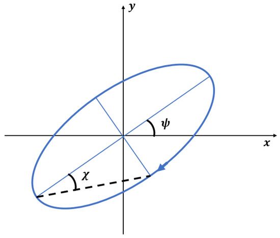
Figure 1.
Sketch of the ellipticity () and orientation () angles defined on the polarisation plane (where x and y can be horizontal, H, and vertical, V, axes). The blue ellipse represents the most general polarisation state of a monochromatic plane electromagnetic wave.
It is worth noting that, when using the Stokes formalism, the partially polarised wave scattered off a distributed target can be uniquely decomposed into a coherent component, i.e., a fully polarised wave with a unitary degree of polarisation (P), and an incoherent component, i.e., a fully unpolarised wave with zero degree of polarisation [33]:
where the SPAN is the total backscattered power measured along all the polarimetric channels:
Note that when a non-zero fully unpolarised component is observed, a random scattering mechanism is in place.
When dealing with the observation of marine vessels using polSAR data, two scattering scenarios must be distinguished: sea surface and vessel. The sea surface scattering can be modelled by the Bragg/tilted Bragg scattering theory [34], for which the backscattered signal is due to the surface roughness whose height is small if compared to the radar wavelength and which is randomly distributed on the scattering surface. In the case of open sea surface observed at intermediate AOI under low-to-moderate wind conditions, low depolarisation is expected. Similarly, the ship/sea contrast changed with the sea roughness; if the sea roughness increases, the ship/sea contrast may decrease because the backscattered return from a rougher sea is higher as compared with a calm sea.
The scattering from a marine vessel significantly depends on the structure and the material the vessel consists of. It is worth expecting that the backscatter from vessels consists of several mechanisms that include: (a) direct reflection from metallic tiles oriented perpendicularly to the radar beam; (b) double backscattering generated by the propagation paths involving sea–ship interactions or the interaction with dihedral structures that may form within the ship; (c) multiple interactions between the electromagnetic wave and sea/ship structures. The random combination of these elementary scattering mechanisms affects both the polarised and unpolarised parts of the scattered wave. The former affects the shape of the polarisation signature, while the latter manifests itself in a pedestal on which the co-polarisation signature is set. The larger the unpolarised component, the larger is the height of the pedestal.
In this study, according to the above-described theoretical background, the polarimetric L-band backscattering from a fishing trawler is analysed when varying the AOI using both incoherent, i.e., multi-polarisation NRCSs and SPAN, and coherent, i.e., normalised co-polarisation signature and PH, scattering descriptors.
3. SAR Dataset
The UAVSAR is an airborne full-polarimetric SAR that operates in the L-band (from 1.2175 GHz to 1.2975 GHz) with a bandwidth of 80 MHz observing a 22 km wide ground swath with an AOI spanning from about to . The noise equivalent sigma zero (NESZ) of the system is −53 dB at mid-range. The UAVSAR has a spatial resolution of 1.7 m × 1 m in range and azimuth direction, respectively. Additional information on the UAVSAR characteristics is provided in Table 1.

Table 1.
UAVSAR operating parameters.
The dataset consists of five UAVSAR SAR scenes collected in the Gulf of Mexico on November 17, 2016, from 15:50 and 17:20 UTC over an area that includes a fishing trawler moving along the range direction from south-west to north-east, see PolSAR flight 16100 in the gulfco_27086 archive [35]. The UAVSAR acquisition geometry is shown in Figure 2. At the time of the SAR acquisitions, the aircraft was flying towards the east direction at an average altitude of about 12.5 km with a heading of approximately , see the red line. Figure 2 also shows the area observed during the UAVSAR acquisition flight, see the light green region, along with the locations of the small ship under investigation through the whole dataset, see the small blue boxes. The latter are labelled according to the AOI at which the ship is observed from the UAVSAR sensor, from lowest (“1”) to highest (“5”). In addition, the traveling direction of the fishing trawler is annotated as a dashed blue arrow. Note that the ship motion has components along both azimuth and range directions, respectively. This high-quality SAR dataset provides a unique opportunity to study the scattering properties of a small ship in a broad range of AOI. According to AIS (Automatic Identification System) information, the fishing trawler under investigation is 20.85 m long and 6.74 m wide. Unfortunately, the image of the fishing trawler under test is not available and, therefore, to get information about its structure and geometry is not possible. In addition, it is worth noting that fishing trawlers may have very different geometries. Nonetheless, as a showcase, a simplified sketch of a fishing trawler is shown in Figure 3. At the time of the UAVSAR flight, the fishing trawler was moving with an average speed of 16 km/h under low sea state conditions, i.e., buoy measurements from PILL1 (29.179N, 89.259W) and PSTL1 (28.932N, 89.407W) NOAA stations provided a wind speed of approximately 5 m/s and a significant wave height lower than 1 m [36].
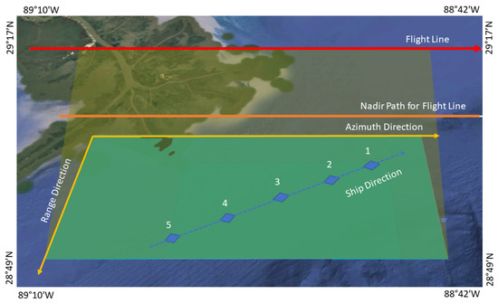
Figure 2.
UAVSAR acquisition geometry. The flight line is depicted in red, while the observed area is shown as a light green patch. The ship location in the five SAR scenes is highlighted by the blue boxes, while its motion is depicted with the dashed blue arrow. The blue boxes are labeled from “1” to “5” that correspond to SAR acquisition at the lowest and highest AOI, respectively.
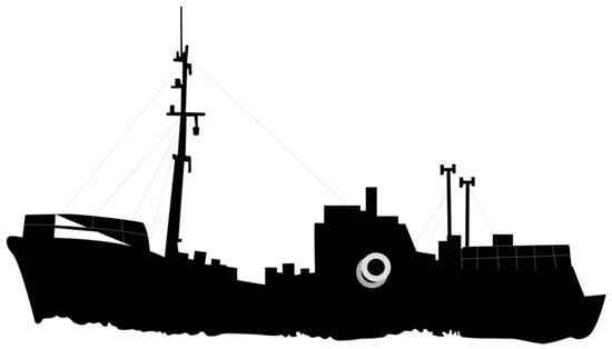
Figure 3.
Simplified sketch of a typical fishing trawler [37].
In this study, the multi-looked complex (MLC) polSAR covariance matrix with (range × azimuth) looks is considered. According to [38], the relationship between the range pixel and the AOI is provided in Figure 4, where the AOI associated with the fishing trawler observed in the five UAVSAR images are also annotated along with the corresponding UTC time. It results that the fishing trawler under investigation was observed by UAVSAR during a time period of about 90 min with an AOI that spans from approximately 35 to about 50. The false colour Pauli-coded UAVSAR images related to the SAR scenes collected at the lowest and highest AOI (see labels “1” and “5” in Figure 2 and Figure 4, respectively) are shown in Figure 5a,b, respectively. They show a coastal area (the Louisiana coast on the northwestern corner) where some large dark features at sea are visible together with several ships that appear as spots brighter than the background sea. The location of the fishing trawler under investigation is highlighted in both images within the white ellipse, where the corresponding AOI is also annotated. Note how, during the two acquisitions, whose time span is about 90 min, the small ship moved from north-east to south-west, see also Figure 2. An inset showing an enlarged version of the Pauli images focused on the fishing trawler under analysis is also included, where differences can be observed in the sea surface and fishing trawler signatures relevant to the lowest and highest AOI, suggesting that further investigation is needed. It is worth noting that the multi-polarisation backscattering properties of a target depend, among all, on its relative orientation with respect to SAR observation direction. Hence, since we are interested in analysing the relationship between the small ship scattering properties and the AOI, i.e., the true heading of the fishing trawler must be first estimated. This information is depicted in Figure 6, where a mosaic image is used as the background image by merging the area that includes the ship excerpted from the five Pauli images. The true heading is represented by straight lines with different colours that connect the fishing trawler position in each sub-image of the mosaic. It can be noted that, during the UAVSAR acquisition flight, the ship kept its true heading constant (about 70) and, therefore, changes in its multi-polarisation backscattering properties are likely to be attributed to variations in the AOI, i.e., to the fishing trawler motion component along the range direction.
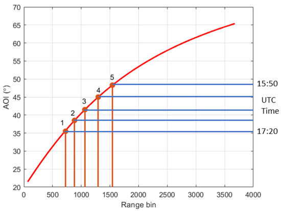
Figure 4.
AOI versus range bin for the UAVSAR geometry. The AOI corresponding to the small ship to be analysed and the SAR acquisition UTC times are also annotated.
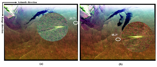
Figure 5.
False colour Pauli image related to the UAVSAR scenes collected at the: (a) lowest and (b) highest AOI. The fishing trawler under investigation, enclosed in the white ellipse, is highlighted in the zoomed-in version of the image.
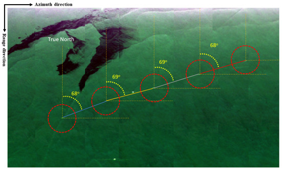
Figure 6.
Estimated heading of the fishing trawler annotated on a mosaic composed by the Pauli images excerpted from the whole UAVSAR dataset.
4. Experiments
In this section, the variability of multi-polarisation scattering of the fishing trawler with respect to AOI is analysed. The surrounding sea surface is also considered as a reference scattering scenario. To this purpose, two equal-size ( pixels in range and azimuth directions, respectively) regions of interest (ROIs) are excerpted over the small ship under investigation and sea surface at the same AOI for each SAR scene of the UAVSAR dataset. The polarimetric scattering analysis includes both incoherent and coherent polarimetric descriptors. The former consist of the multi-polarisation NRCSs (HH, HV and VV channels) and the SPAN, while the latter are the co-polarised signature and the PH. To assess the degree of separability between ship and sea signals, the TCR metric in dB scale is used, which is defined as [21,39]:
where X∈ {, , , SPAN, PH} is the mean value of the feature evaluated within the ROI excerpted over the fishing trawler (subscript t) and the sea surface (subscript s), respectively.
The first experiment is to analyse the incoherent scattering descriptors, i.e., the multi-polarisation NRCSs and the SPAN, evaluated over the sea surface and the ship under investigation at the five AOIs, see Figure 7, where the mean values evaluated over the sea (dashed lines) and ship (continuous lines) ROIs are shown. The corresponding mean values are also listed in Table 2. When dealing with the reference sea surface, it can be noted that typical signatures of Bragg/tilted-Bragg surface scattering applies. The latter results in the largest VV-polarised backscattering (blue plot) and a cross-polarised NRCS (red plot) which is significantly lower, i.e., from about 10 dB to 20 dB, than the co-polarised backscattering channels. In addition, the NRCSs all decrease with AOI due to the fact that, when increasing AOI, the sea surface roughness is responsible of a scattered signal mainly directed towards the forward direction rather than towards the backward direction where the SAR antenna is placed. As a result, the HV-, VV-, and HH-polarised (see black plot) backscattered signals are—at the highest AOI, i.e., approximately 48—about 1.6 dB, 2.5 dB, and 6.6 dB, respectively, lower than that their corresponding values at the lowest AOI, i.e., about 36.
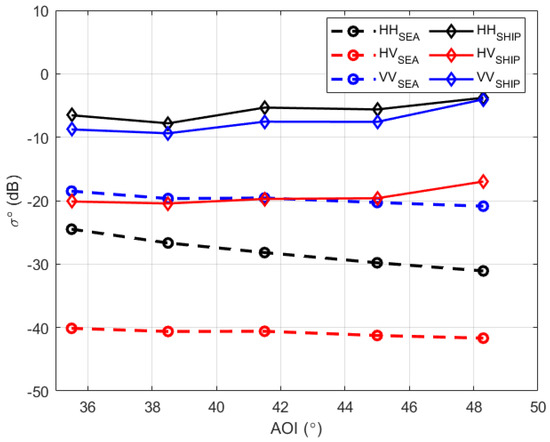
Figure 7.
Average multi–polarisation NRCSs with respect to AOI. Dashed lines with circle markers and continuous lines with diamond markers refer to sea and ship ROIs, respectively, while black, red, and blue colours refer to HH, HV, and VV polarisation, respectively. The dB scale is adopted.
Table 2.
Mean values (in dB) of incoherent scattering descriptors, i.e., multi-polarisation NRCSs and SPAN, evaluated over both sea and ship ROIs at the five AOIs.
When dealing with the backscattering of the fishing trawler, a different behaviour is in place. The metallic structure of the ship results in a backscattered signal much larger than the sea surface one, see the NRCSs continuous plots which are at least about 10 dB higher than the corresponding continuous curves. This behaviour is emphasized when dealing with the cross-polarised NRCS that, due to the complicated structure of the ship giving rise to multiple and helix scattering mechanisms, shows backscattering values 20 dB larger than the sea surface ones at any AOI. However, although even in this case, the co-polarised backscattering is much larger than the cross-polarised one (about 12 dB difference), the largest NRCS is observed for the HH channel. The NRCSs also show a non-negligible increasing trend (approximately from 2.5 dB to 5 dB variation) with AOI.
Once the behaviour of multi-polarisation NRCSs is analysed with respect to AOI, the SPAN is considered whose results are depicted in Figure 8, where (a) and (b) refer to sea surface and fishing trawler ROIs, respectively. The corresponding mean values are also listed in Table 2. When dealing with sea surface, see Figure 8a, a low SPAN is observed at all AOIs that lie in a 3 dB range from about −20.5 dB up to −17.5 dB. This is due to the actual low sea state conditions at the time of the UAVSAR flight which result in moderate surface roughness and to the L-band dielectric properties of sea surface. In addition, as expected from the Bragg/tilted-Bragg scattering theory, the SPAN is characterised by a decreasing trend with AOI.
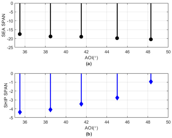
Figure 8.
SPAN evaluated at the five AOIs for: (a) sea and (b) ship ROIs. The dB scale is used.
With reference to the fishing trawler, it must be pointed out that a different scattering behaviour applies in terms of the total backscattered power, see Figure 8b. First, it can be noted that the metallic material the ship consists of and its complex geometric structure result in a much larger SPAN, spanning from about −4.5 dB up to −1 dB, with respect to sea surface (see Table 2). This is why the fishing trawler appears as a bright spot in the Pauli images of Figure 5. In addition, the SPAN of the fishing trawler exhibits an increasing trend with AOI. Given the relative orientation between the ship and the SAR look direction, this behaviour can be likely attributed to the fact that, when increasing AOI, the scattering surfaces responsible of the signal scattered off the fishing trawler are mostly oriented, on average, towards the backward direction and, therefore, a larger part of the incident electromagnetic wave is scattered off towards the SAR antenna. It is also worth noting that the same absolute SPAN variation, i.e., about 3 dB, applies over both sea and ship ROIs when moving from the lowest to the highest AOI. Results shown in Figure 8 suggest to further investigate the behaviour of the incoherent scattering descriptors when the AOI changes.
To this aim, to better understand the relative contribution of the single polarimetric scattering channels to the SPAN, a second experiment is undertaken that consists of evaluating the behaviour of multi-polarisation NRCSs, normalised to the SPAN, versus the AOI. Results are shown in Figure 9 for the five AOIs and for both sea surface and fishing trawler ROIs. In Figure 9a–c, the symbols refer to the relative scattering contribution of HH-, HV-, and VV-polarised NRCS, while black and blue colours refer to sea and ship ROI, respectively.
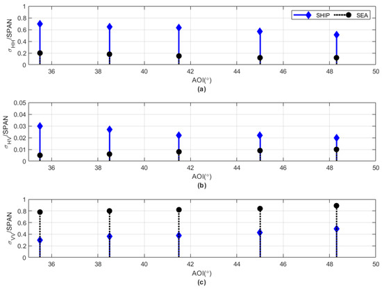
Figure 9.
Relative contribution to the SPAN of multi-polarisation NRCSs evaluated over sea (black) and ship (blue) ROIs. (a): HH-, (b) HV-, and (c) VV-polarised NRCS. The linear scale is adopted.
When dealing with the reference sea surface, as expected from the Bragg scattering theory, the dominant contribution to the signal scattered off sea surface is provided by the VV channel that contributes no less than 80% of the SPAN. The other relevant scattering contribution, ranging from about 10% to 20%, comes from the HH channel, while the cross-polarised contribution is negligible, i.e., no larger than 2%, at all AOIs. This is due to the non-depolarising nature of sea surface scattering that results in a negligible cross-polarised backscattered signal. In Figure 9, it can be also observed that the relative contribution to the total backscattering of the HH-polarised NRCS decreases with AOI, while this is no longer the case of HV and VV channels, which increase with AOI. In fact, while the relative contribution of the VV-polarised NRCS to the SPAN moves from approximately 80% to about 90%, the corresponding contribution related to the HH channels decreases from about 20% down to approximately 10%. This means that, in the L-band, observing the sea surface under low-to-moderate conditions while moving from 35 to 49 results in about 10% of the total backscattered power switching from HH to VV polarisation.
With reference to the fishing trawler under investigation, a completely different scattering behaviour is observed, see blue plots in Figure 9. If the variability of sea surface backscattering with AOI is marginal, overall, this is no longer the case of the ship, which exhibits significant changes in backscattering when varying AOI. This must be attributed to the fact that, differently from the sea surface case, the structure of the ship is composed by surfaces with different orientations, vertical structures, dihedral scatterers, etc., making the backscattered signal much more sensitive to changes in the observation geometry, i.e., AOI. The total backscattered power is ruled by the HH-polarisation, which represents at least 50% of the SPAN at all AOIs. As for the sea surface case, the cross-polarised contribution provides the lowest contribution to the SPAN (i.e., no larger than 3%), even if, given an AOI, the relative contribution of the HV-polarised NRCS of the ship is about 2 (at about 48)—6 (at approximately 36) times larger than that of the corresponding sea contribution. With respect to sea surface, over the fishing trawler, the backscattering contribution of the co-polarised channels is more balanced since no dominant scattering mechanism is in place. Considering the trend of the normalised multi-polarisation NRCSs with AOI, it must be noted that HH- and HV-polarised channels decrease when increasing AOI, while the VV-polarised contribution increases with AOI, see Figure 9c. Considering that co-polarised backscattering dominates over both sea surface and fishing trawler (see Figure 7) and that here the relative contribution provided by the different polarimetric channels is shown once the total backscattered power is given, it is expected that the difference between HH- and VV-polarised NRCS as well as their relative contribution to the backscattered energy change with AOI. In particular, when AOI increases, we found that part of backscattered energy measured in the HH channel is converted into the VV channel. When dealing with the dominant co-polarised channels over the ship, their relative contribution tends to get closer when the AOI increases. In fact, if the relative contribution at about 36 is approximately 70% and 30% for HH and VV channels, it changes into about 55% and 45%, respectively, at approximately 48. This means that at highest AOI, the total backscattering from the fishing trawler is equally split into the co-polarised channels.
A joint analysis of Figure 8 and Figure 9 shows that the decreasing trend with AOI of the sea surface SPAN (see Figure 8a) is due to the relative contribution of the HH channel that decreases with increasing AOI, see Figure 9a. Similarly, the fishing trawler SPAN that increases with AOI is mostly due to the increasing contribution of the VV channel with AOI, see Figure 9c. To quantitatively discuss those insights, the relative contribution of multi-polarisation NRCSs to the SPAN is evaluated, for the five AOIs, as the percentage change (PC) between ship and sea ROI backscattering, according to the following metrics:
where the subscript X refers either to HH- and HV-polarised channel, while the subscript V refers to the VV-polarised channel. The different definition of the PC metric for the VV channel is due to the fact that the relative contribution of the VV-polarised sea surface backscattering is larger than the ship one, while this is no longer the case of HH- and HV-polarised signals (see Figure 9c). In (10), the NRCSs represent the mean value evaluated within the ROI excerpted over the fishing trawler (subscript t) and the sea surface (subscript s), respectively. The results, listed in Table 3, confirm the significant dependence of the backscattering to the AOI. The PC of ship to sea relative backscattering reduces for all the polarimetric channels when AOI increases from about 36 to approximately 48. In particular, spanning the considered AOI range, reduces from about 76% down to approximately 65%, while decreases from approximately 82% to about 52%. The VV channel exhibits the lowest variability with AOI, since slightly reduces from 45% down to 40.5% when increasing AOI.
Table 3.
Multi-polarisation PC metrics evaluated at the five AOIs.
The third experiment consists of analysing the ship/sea backscattering separability at different AOIs according to the TCR metric, see (9). Experimental results are shown in Figure 10, where the dB scale is adopted and where black, red, and blue lines refer to HH-, HV-, and VV-polarised TCR, respectively. The corresponding values are also listed in Table 4 for the five AOIs. It can be pointed out that the TCR increases with AOI independently on the polarisation, meaning that when single-polarisation NRCSs are considered for ship detection, higher AOIs should be preferred since they show a better separability between sea surface and fishing trawler backscattering. Experimental results also show that the VV-polarised channel provides the lowest TCR values (i.e., from about 9 dB at approximately 36 up to about 17 dB at approximately 48) at all AOIs. This is due to the fact that, as witnessed by the previous experiments, the VV channel provides the largest sea surface backscattering, therefore resulting in a reduced TCR, see (9). In addition, the TCR plots depicted in Figure 10 also show that a non-negligible AOI-dependent difference (no larger than 3 dB) applies for HH- and HV-polarised TCR. In fact, at lower (higher) AOIs, i.e., AOI <40 (AOI >40), the HV channel results in a TCR larger (lower) than the HH one. This finding agrees with the outcomes observed in [7].
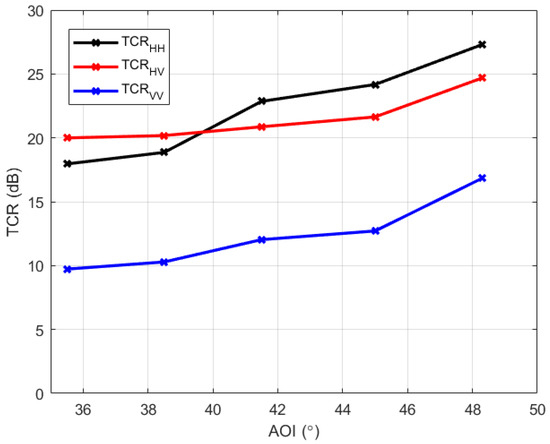
Figure 10.
TCR versus AOI for different polarisations. Black, red, and blue plots refer to the HH-, HV-, and VV-polarised channels.
Table 4.
Mean TCR values (in dB) estimated for the multi-polarisation NRCSs at the five AOIs.
The fourth experiment is to analyse the coherent scattering descriptors, i.e., the normalised co-polarisation signatures and PH, evaluated over the sea surface and the ship under investigation at the five AOIs. The normalised co-polarisation signatures estimated over the sea surface and ship ROIs are shown in Figure 11 and Figure 12, respectively.
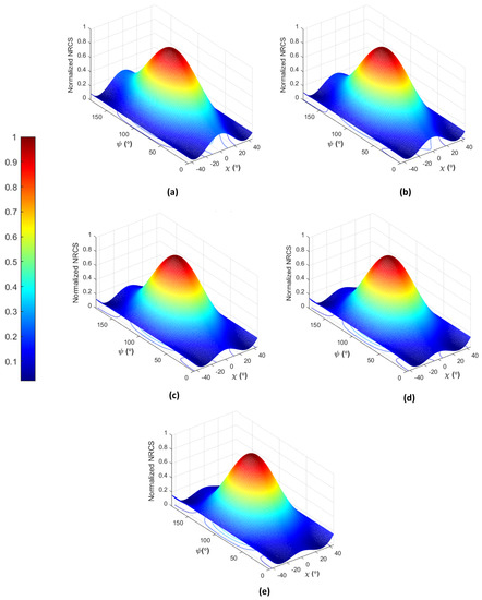
Figure 11.
Normalised co–polarisation signature evaluated over the sea surface ROI at: (a) AOI = 35.7, (b) AOI = 38.5, (c) AOI = 41.5, (d) AOI = 45, (e) AOI = 48.3.
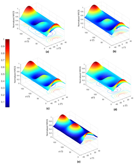
Figure 12.
Normalised co–polarisation signature evaluated over the fishing trawler ROI at: (a) AOI = 35.7, (b) AOI = 38.5, (c) AOI = 41.5, (d) AOI = 45, and (e) AOI = 48.3.
With reference to the sea surface, the normalised co-polarisation signature depicted in Figure 11 shows that the shape of signature does not change with AOI. In fact, the normalised co-polarisation signature is characterised by the well-known Bragg shape at all the AOIs [29,40]. This leads to the typical signature of sea surface scattering according to the Bragg theory, i.e., largest backscattering at VV polarisation ( = 0, = 90), lowest backscattering close to circular polarisations ( = ± 45, ∀), and low amount of unpolarised backscattered energy (i.e., low PH). Only small differences can be observed in the normalised co-polarisation signature of the sea surface when the AOI increases, see the slight increase in the PH and the small reduction in the HH-polarised relative backscattering ( = 0, = 0, 180). This confirms the result shown in Figure 9.
When dealing with the normalised co-polarisation signature of the fishing trawler, see Figure 12, a very different shape is in place if compared to the sea surface one. First, it must be pointed out that the shape of the ship’s signature is by far more complicated than that the Bragg-like one characterising the sea surface, since it results from the combination of different elementary scattering mechanisms whose relative contribution depends on several factors (e.g., the relative orientation of the scattering structures the ship consist of with respect to the SAR look direction, the materials these structures are made of, etc.). Nonetheless, even if a non-negligible sensitivity to AOI can be noted for the ship’s signature, some peculiar features of the backscattering from the fishing trawler are clearly observed. First, it can be noted that the normalised co-polarisation signature has maxima at HH polarisation (i.e., = 0 and = 0/180, see Figure 1), regardless the AOI. This agrees with the results observed in Figure 9, demonstrating that, given the acquisition geometry, the largest backscattering for the fishing trawler under analysis occurs when horizontal polarisation is transmitted while receiving in horizontal polarisation. A local maximum can be observed at VV polarisation (i.e., = 0, = 90, see Figure 1) at any AOI, whose value increases with AOI. At the highest AOI, see Figure 12e, the relative contribution of the VV-polarised backscattering over the fishing trawler results in almost the same observed for the HH channel, as suggested in Figure 9a,c. In addition, it can be noted that the fishing trawler backscattering shows a PH much larger than the one that characterises the sea surface, and that it slightly increases with AOI. This is likely due to the fact that the complex scattering process that characterises the fishing trawler leads to a random combination of helix, single-, double-, and multiple-bounce elementary scattering mechanisms that, in turn, results in an increase of the unpolarised component of the backscattered signal measured at the SAR antenna.
To better quantify the variation of the PH with respect to AOI, it is evaluated for both sea and ship ROIs. Results are depicted in Figure 13 with black and blue lines, respectively, using a dB scale. The corresponding values are also listed in Table 5. As qualitatively observed in Figure 11 and Figure 12, the fishing trawler is characterised by PH values quite larger than that of the sea surface, while in both cases, the PH increases with AOI. Considering the sea surface, the amount of unpolarised energy is almost stable at lower AOIs (AOI < 42), i.e., about −19 dB, while it slightly increases of about 1 dB at higher AOIs (AOI > 42). With reference to the ship, the PH increases of about 3 dB when the AOI increases from approximately 36 to 48, i.e., it spans from −13.3 dB up to −10.7 dB. Figure 13 also shows the corresponding TCR evaluated from the PH, see the red plot, whose values are also listed in Table 6 for the five AOIs. Since the difference between sea and ship PH keeps almost constant with AOI, the TCR does not change significantly when increasing AOI, settling close to 6–7 dB. This demonstrates that the polarised component of the backscattered signal is more sensitive to AOI if compared to the unpolarised one.
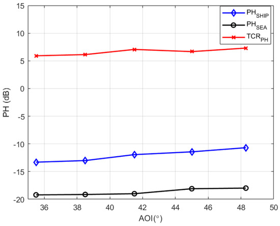
Figure 13.
Behaviour of the PH and its corresponding TCR. Black and blue lines refer to sea and ship ROIs, while the red plot refers to the TCR. The dB scale is adopted.
Table 5.
Mean PH values (in dB) evaluated over both sea and ship ROIs at the five AOIs.
Table 6.
Mean TCR values (in dB) estimated for the PH at the five AOIs.
5. Conclusions
This study deals with the observation of ships by means of polarimetric synthetic aperture radar. Advanced ship detection and classification approaches have been proposed that exploit the different scattering properties of the marine vessels with respect to the surrounding sea. Nevertheless, it is well-established that the detectability of the ships depends on several factors, including the incident wavelength and the angle of incidence of the synthetic aperture radar sensor, the sea state conditions at the acquisition time, the characteristics of the ship to be observed such as the size, the heading, the structure, the material it consists of.
Hence, in this study, we analyse the effects of the incidence angle on the polarimetric backscattering properties of a small ship. To this aim, the scattering from a fishing trawler is analysed by means of a unique dataset composed by five L-band UAVSAR airborne synthetic aperture radar scenes collected in full-polarimetric imaging mode. This premium dataset offered the chance to investigate, for the first time, changes in polarimetric scattering properties of a same small ship when observed under the same sea state conditions but in a wide range of incidence angles, i.e., from about 35–50. The analysis is performed on both polarised and unpolarised components of the backscattered signal according to coherent, i.e., co-polarisation signature and pedestal height, and incoherent, i.e., multi-polarisation NRCSs and SPAN, scattering descriptors.
With reference to the polarised scattering component, the experiments point out that the scattering from the small ship is ruled by HH polarisation (>70% of the SPAN) at lower incidence angles while both co-polarised channels equally contribute to the total backscattered power at higher incidence angles. In addition, we found that the HH channel provides the largest target-to-clutter ratio (>20 dB) at higher incidence angles, i.e., >40, while at lower incidence angles (<40), the HV channel is the one that results in the largest target-to-clutter ratio, i.e., around 20 dB. With respect to the unpolarised scattering component, experimental results show that it is less sensitive to the incidence angle, i.e., the amount of unpolarised energy scattered off the small ship under analysis does not change significantly with incidence angle, therefore resulting in a target-to-clutter ratio which is remarkably lower (<7 dB) than that of the single-polarisation backscattering power (>10 dB if the worst channel, i.e., VV is considered), especially at higher incidence angles.
It must be explicitly pointed out that those outcomes are closely related to the specific experimental configuration and, therefore, different conditions as shorter incident wavelengths, larger ships or ships characterised by different structures, higher sea state conditions may lead to different results. Nonetheless, even though nowadays most of the algorithms for ship detection and classification are based on the different scattering properties that characterise the ships with respect to the background sea, the effects the incidence angles have on the multi-polarisation backscattering are not taken into account. Hence, the outcomes presented in this study aim at shedding light on how the scattering properties of a small ship change when the target is observed under different incidence angles. This may be helpful when robust and effective ship detection and classification algorithms are intended to be developed, i.e., by suggesting the parameter that provides the larger TCR according to the incidence angle at which the actual ship is observed by the SAR. In the future, a similar multi-polarisation scattering analysis could be undertaken by including more descriptors, i.e., the degree of polarisation, and extended to different experimental conditions, i.e., a polSAR sensor operating at shorter wavelengths, higher sea states, etc., as long as a similar SAR dataset collected on a ground-truthed ship observed under a wide range of incidence angles is available.
Author Contributions
Conceptualizationmethodology, A.B. and F.N.; software, M.A. and E.F.; validation, M.A., A.B. and E.F.; formal analysis, A.B. and F.N.; data curation, M.A. and D.V.; writing—original draft preparation, A.B. and M.M.; writing—review and editing, A.B., F.N. and M.M; supervision, F.N., D.V. and M.M. All authors have read and agreed to the published version of the manuscript.
Funding
This research received no external funding.
Data Availability Statement
Not applicable.
Acknowledgments
Thanks to the European Space Agency (ESA) for funding this study under the framework of the Dragon 5 cooperation project ID 57979 “Monitoring harsh Coastal environments and Ocean Surveillance using radar remote sensing sensors”. Thanks to the National Aeronautics and Space Administration Jet Propulsion Laboratory for providing UAVSAR data free of charge.
Conflicts of Interest
The authors declare no conflict of interest.
Abbreviations
The following abbreviations are used in this manuscript:
| AIRSAR | AIRborne SAR |
| AIS | Automatic Identification System |
| ALOS | Advanced Land Observing Satellite |
| AOI | Angle Of Incidence |
| CFAR | Constant False Alarm Rate |
| dB | deciBel |
| ESA | European Space Agency |
| HH | Horizontal transmit Horizontal receive |
| HV | Horizontal transmit Vertical receive |
| JPL | Jet Propulsion Laboratory |
| MLC | Multi-Looked Complex |
| NASA | National Aeronautics and Space Administration |
| NESZ | Noise Equivalent Sigma Zero |
| NOAA | National Oceanic and Atmospheric Administration |
| NRCS | Normalised Radar Cross Section |
| PALSAR | Phased Array type L-band SAR |
| PC | Percentage Change |
| PH | Pedestal Height |
| PolSAR | Polarimetric SAR |
| ROI | Region Of Interest |
| SAR | Synthetic Aperture Radar |
| SIR | Spaceborne Imaging Radar |
| TCR | Target-to-Clutter Ratio |
| UAVSAR | Uninhabited Aerial Vehicle Synthetic Aperture Radar |
| UTC | Universal Time Coordinated |
| VV | Vertical transmit Vertical receive |
References
- CLEANSEANET Service European Maritime Safety Agency (EMSA). Available online: http://cleanseanet.emsa.europa.eu/ (accessed on 28 July 2022).
- Curlander, J.C.; McDonough, R.N. Synthetic Aperture Radar; Wiley: New York, NY, USA, 1991. [Google Scholar]
- Souyris, J.C.; Henry, C.; Adragna, F. On the use of complex SAR image spectral analysis for target detection: Assessment of polarimetry. IEEE Trans. Geosci. Remote Sens. 2003, 41, 2725–2734. [Google Scholar] [CrossRef]
- Migliaccio, M.; Nunziata, F.; Montuori, A.; Paes, R.L. Single-look complex COSMO-SkyMed SAR data to observe metallic targets at sea. IEEE J. Selected Topics Appl. Earth Obs. Remote Sens. 2012, 5, 893–901. [Google Scholar] [CrossRef]
- Margarit, G.; Mallorqui, J.J.; Fortuny-Guasch, J.; López-Martínez, C. Phenomenological vessel scattering study based on simulated inverse SAR imagery. IEEE Trans. Geosci. Remote Sens. 2009, 47, 1212–1223. [Google Scholar] [CrossRef]
- Stefanowicz, J.; Ali, I.; Andersson, S. Current trends in ship detection in single polarization synthetic aperture radar imagery. In Proceedings of the Photonics Applications in Astronomy, Communications, Industry, and High Energy Physics Experiments 2020, Wilga, Poland, 31 August–2 September 2020; Volume 11581, pp. 66–77. [Google Scholar]
- Crisp, D.J. The State-of-the-Art in Ship Detection in Synthetic Aperture Radar Imagery; Technical report; Defence Science And Technology Organisation Salisbury: Canberra, Australia, 2004. [Google Scholar]
- Liu, T.; Zhang, J.; Gao, G.; Yang, J.; Marino, A. CFAR ship detection in polarimetric synthetic aperture radar images based on whitening filter. IEEE Trans. Geosci. Remote Sens. 2019, 58, 58–81. [Google Scholar] [CrossRef]
- Chen, J.; Chen, Y.; Yang, J. Ship detection using polarization cross-entropy. IEEE Geosci. Remote Sens. Lett. 2009, 6, 723–727. [Google Scholar] [CrossRef]
- Migliaccio, M.; Nunziata, F.; Montuori, A.; Li, X.; Pichel, W.G. A multifrequency polarimetric SAR processing chain to observe oil fields in the Gulf of Mexico. IEEE Trans. Geosci. Remote Sens. 2011, 49, 4729–4737. [Google Scholar] [CrossRef]
- Ferrara, G.; Migliaccio, M.; Nunziata, F.; Sorrentino, A. GK-based observation of metallic targets at sea in full-resolution SAR data: A multipolarization study. IEEE J. Ocean. Eng 2011, 36, 195–204. [Google Scholar] [CrossRef]
- Marino, A. A notch filter for ship detection with polarimetric SAR data. IEEE J. Selected Topics Appl. Earth Obs. Remote Sens. 2013, 6, 1219–1232. [Google Scholar] [CrossRef]
- Zhang, T.; Yang, Z.; Gan, H.; Xiang, D.; Zhu, S.; Yang, J. PolSAR ship detection using the joint polarimetric information. IEEE Trans. Geosci. Remote Sens. 2020, 58, 8225–8241. [Google Scholar] [CrossRef]
- Iervolino, P.; Guida, R.; Lumsdon, P.; Janoth, J.; Clift, M.; Minchella, A.; Bianco, P. Ship detection in SAR imagery: A comparison study. In Proceedings of the 2017 IEEE International Geoscience and Remote Sensing Symposium (IGARSS), Fort Worth, TX, USA, 23–28 July 2017; pp. 2050–2053. [Google Scholar]
- Yin, J.; Yang, J.; Zhou, Z.S.; Song, J. The Extended Bragg Scattering Model-Based Method for Ship and Oil-Spill Observation Using Compact Polarimetric SAR. IEEE J. Selected Topics Appl. Earth Obs. Remote Sens. 2015, 8, 3760–3772. [Google Scholar] [CrossRef]
- Xu, X.; Zhang, X.; Zhang, T. Lite-yolov5: A lightweight deep learning detector for on-board ship detection in large-scene sentinel-1 sar images. Remote Sens. 2022, 14, 1018. [Google Scholar] [CrossRef]
- Zhang, T.; Zhang, X.; Shi, J.; Wei, S. HyperLi-Net: A hyper-light deep learning network for high-accurate and high-speed ship detection from synthetic aperture radar imagery. ISPRS J. Photogramm. Remote Sens. 2020, 167, 123–153. [Google Scholar] [CrossRef]
- Zhang, T.; Zhang, X. A mask attention interaction and scale enhancement network for SAR ship instance segmentation. IEEE Geosci. Remote Sens. Lett. 2022, 19, 1–5. [Google Scholar] [CrossRef]
- Zhang, T.; Zhang, X.; Liu, C.; Shi, J.; Wei, S.; Ahmad, I.; Zhan, X.; Zhou, Y.; Pan, D.; Li, J.; et al. Balance learning for ship detection from synthetic aperture radar remote sensing imagery. ISPRS J. Photogramm. Remote Sens. 2021, 182, 190–207. [Google Scholar] [CrossRef]
- Zhang, T.; Zhang, X. A polarization fusion network with geometric feature embedding for SAR ship classification. Pattern Recognit. 2022, 123, 108365. [Google Scholar] [CrossRef]
- Yeremy, M.; Campbell, J.; Mattar, K.; Potter, T. Ocean surveillance with polarimetric SAR. Can. J. Remote. Sens. 2001, 27, 328–344. [Google Scholar] [CrossRef]
- Touzi, R.; Charbonneau, F.; Hawkins, R.; Vachon, P. Ship detection and characterization using polarimetric SAR. Can. J. Remote. Sens. 2004, 30, 552–559. [Google Scholar] [CrossRef]
- Touzi, R.; Hurley, J.; Vachon, P.W. Optimization of the degree of polarization for enhanced ship detection using polarimetric RADARSAT-2. IEEE Trans. Geosci. Remote Sens. 2015, 53, 5403–5424. [Google Scholar] [CrossRef]
- Guissard, A. Mueller and Kennaugh matrices in radar polarimetry. IEEE Trans. Geosci. Remote Sens. 1994, 32, 590–597. [Google Scholar] [CrossRef]
- Van Zyl, J.; Papas, C.; Elachi, C. On the optimum polarizations of incoherently reflected waves. IEEE Trans. Antennas. Propag. 1987, 35, 818–825. [Google Scholar] [CrossRef]
- Gil, J.J. Characteristic properties of Mueller matrices. JOSA A 2000, 17, 328–334. [Google Scholar] [CrossRef]
- Cloude, S. Polarisation: Applications in Remote Sensing; OUP Oxford: Oxford, UK, 2009. [Google Scholar]
- Zebker, H.A.; Van Zyl, J.J.; Held, D.N. Imaging radar polarimetry from wave synthesis. J. Geophys. Res. Solid Earth 1987, 92, 683–701. [Google Scholar] [CrossRef]
- Nunziata, F.; Migliaccio, M.; Gambardella, A. Pedestal height for sea oil slick observation. IET Radar Sonar Navig. 2010, 5, 103–110. [Google Scholar] [CrossRef]
- Buono, A.; Nunziata, F.; Migliaccio, M. Analysis of Full and Compact Polarimetric SAR Features Over the Sea Surface. IEEE Geosci. Remote Sens. Lett. 2016, 13, 1527–1531. [Google Scholar] [CrossRef]
- Buono, A.; Nunziata, F.; Migliaccio, M.; Li, X. Polarimetric Analysis of Compact-Polarimetry SAR Architectures for Sea Oil Slick Observation. IEEE Trans. Geosci. Remote Sens. 2016, 54, 5862–5874. [Google Scholar] [CrossRef]
- Shirvany, R.; Chabert, M.; Tourneret, J.Y. Ship and oil-spill detection using the degree of polarization in linear and hybrid/compact dual-pol SAR. IEEE J. Selected Topics Appl. Earth Obs. Remote Sens. 2012, 5, 885–892. [Google Scholar] [CrossRef]
- Evans, D.L.; Farr, T.G.; Van Zyl, J.J.; Zebker, H.A. Radar polarimetry: Analysis tools and applications. IEEE Trans. Geosci. Remote Sens. 1988, 26, 774–789. [Google Scholar] [CrossRef]
- Valenzuela, G.R. Theories for the interaction of electromagnetic and oceanic waves—A review. Bound.-Layer Meteorol. 1978, 13, 61–85. [Google Scholar] [CrossRef]
- NASA. Gulf Coast, Mexico. 2016. Available online: https://uavsar.jpl.nasa.gov/cgi-bin/data.pl (accessed on 17 June 2022).
- NDBC. Gulf of Mexico (West). 2016. Available online: https://www.ndbc.noaa.gov/obs.shtml (accessed on 10 July 2022).
- PDP. Sketch of a Fishing Trawler. 2022. Available online: https://www.publicdomainpictures.net/en/view-image.php?image=118770&picture=english-trawler (accessed on 25 October 2022).
- Minchew, B.; Jones, C.E.; Holt, B. Polarimetric analysis of backscatter from the Deepwater Horizon oil spill using L-band synthetic aperture radar. IEEE Trans. Geosci. Remote Sens. 2012, 50, 3812–3830. [Google Scholar] [CrossRef]
- Touzi, R.; Goze, S.; Le Toan, T.; Lopes, A.; Mougin, E. Polarimetric discriminators for SAR images. IEEE Trans. Geosci. Remote Sens. 1992, 30, 973–980. [Google Scholar] [CrossRef]
- Van Zyl, J.J.; Zebker, H.A.; Elachi, C. Imaging radar polarization signatures: Theory and observation. Radio Sci. 1987, 22, 529–543. [Google Scholar] [CrossRef]
Publisher’s Note: MDPI stays neutral with regard to jurisdictional claims in published maps and institutional affiliations. |
© 2022 by the authors. Licensee MDPI, Basel, Switzerland. This article is an open access article distributed under the terms and conditions of the Creative Commons Attribution (CC BY) license (https://creativecommons.org/licenses/by/4.0/).