Article

Analysis of the Spatial and Temporal Patterns of Ground-Level Ozone Concentrations in the Guangdong–Hong Kong–Macao Greater Bay Area and the Contribution of Influencing Factors

1
Key Laboratory for Urban Habitat Environmental Science and Technology, School of Urban Planning and Design, Peking University, Shenzhen 518055, China
2
Laboratory for Earth Surface Processes, Ministry of Education, College of Urban and Environmental Sciences, Peking University, Beijing 100871, China
*
Author to whom correspondence should be addressed.
Remote Sens. 2022, 14(22), 5796; https://doi.org/10.3390/rs14225796
Submission received: 26 October 2022 / Revised: 11 November 2022 / Accepted: 15 November 2022 / Published: 16 November 2022

Abstract

:
Ozone (O3) pollution has negative impacts on human health and property. The Guangdong–Hong Kong–Macao Greater Bay Area (GBA) is facing severe O3 pollution problems due to rapid economic development. In this paper, we used sensitivity experiments and GeoDetector to analyze the effects of meteorological factors, anthropogenic emissions, and landscape patterns on O3 concentrations as well as the contributions of NOx and NMVOC (non-methane volatile organic compounds) to the variation of O3 concentrations and the causes of sectoral emissions in the GBA in 2017. The results revealed that, in GBA, the contribution of meteorology to the variation of O3 concentration was dominant both in terms of region and extent, and the contribution of emissions was relatively weak. The contribution of meteorology and emissions to O3 production was mainly contributory. Meteorology contributed significantly to O3, and its non-linear interaction with anthropogenic emissions and surface landscape affected O3 concentration changes. The degree of contribution of NOx and NMVOC varied widely among seasons, and the variation of their relative contribution areas was related to residential sector emissions and agricultural sector emissions. This article enriches the exploration of the O3 formation mechanism in the GBA and provides theoretical support for the implementation of differentiated regional and seasonal mitigation strategies for O3 concentration.

Graphical Abstract

1. Introduction

Tropospheric ozone (O3) is a component of photochemical smog. Long-term or short-term exposure to O3 will have an impact on pulmonary function and the cardiovascular and nervous systems [1,2], resulting in premature death, the reduction of crop productivity, and economic losses [3,4,5,6]. During 2015–2019, sulfur dioxide (SO2), nitrogen dioxide (NO2), PM (particulate matter), and carbon monoxide (CO) mean annual concentrations in Chinese urban environments showed a downward trend, while the mean annual concentration of O3 increased by 4.7% [7,8,9,10]. Surface O3 pollution has become a major air pollution problem in many cities in developing China [11]. Elucidating the O3 spatial mechanism of generation and dispersion is important for developing effective strategies.
Meteorology is a major aspect driving O3 production [12,13], where temperature, total precipitation, relative humidity, surface pressure, and wind speed are important variables affecting its concentration [14,15,16,17,18]. Surface O3 is formed by complex photochemical reactions involving atmospheric nitrogen oxides (NOx), volatile organic compounds (VOCs), and methane [19]. Due to the complex response of O3 to meteorology and precursor emissions, the influence of these variables (and their interactions) on surface O3 varies significantly with season and region [16,20]. In addition, land use, which reflects the intensity of human activities, also alters the production and cycling characteristics of O3 [14]. However, most current studies on the role of land use on air pollution focus on the effects on particulate matter (PM2.5, PM10) concentrations [21,22,23,24], and there are fewer studies on the effects of land use landscape patterns on O3.
Sensitivity experiments are often used in air pollutant analyses, which are simulated by chemical transport models (e.g., the GEOS Chem, WRF-CMAQ model) [12,25,26,27,28]. On the basis of emission inventory and meteorological data, the contribution of factors can be obtained by simulating pollutant concentration values in two or more periods. The neural network is a statistical model prediction method and an effective tool used to describe variation in nonlinear phenomena [29], which is characterized by simple calculations, low data requirements, and high accuracy [30]. Using this method to predict and simulate air pollutants, it is possible to obtain a nonlinear prediction and simulation within a short period, without needing a large amount of meteorological and anthropogenic emission data. Moreover, most of the studies conducted sensitivity experiments over many years or the same period of two years, and there is less seasonal analysis within one year.
Currently, the methods adopted to explore the impact of environmental conditions on the variation of O3 concentration include multiple linear regression [31,32,33], quantile regression [31,33], principal component analysis [32], Kolmogorov–Zurbenko (KZ) filtering [34], and convergence cross-mapping [35]. The GeoDetector method has been widely used to study the interaction among air pollution factors, which could overcome collinearity and quantify the influence of single factors and their interactions [16]. O3 formation involves photochemical reactions and nonlinear responses between most meteorological variables [36,37], primary pollutants such as NOx and VOC [38], and aerosols and O3 [39]. Coupled with the fact that high urban temperature can have direct or indirect effects on O3 and VOC concentrations [40], it becomes increasingly important to investigate the effects of urban O3 concentrations using nonlinear models.
As an important leading region for China’s economic growth, the Guangdong–Hong Kong–Macao Greater Bay Area (GBA) has seen rapid urban development in recent years, followed by increasing ground-level O3 pollution [41]. This paper investigates the seasonal dominant factors affecting the ground O3 in the GBA and explores the effects of meteorological variables, anthropogenic emissions variables, and landscape patterns on the O3 concentration. In this paper, we first designed four sets of sensitivity experiments based on the back propagation (BP) neural network to identify the dominant factors in different seasons and explored the sensitivity zoning of NOx and NMVOC affecting O3. Then, the GeoDetector model was used to quantify the contribution of anthropogenic emissions, meteorological variables, and landscape patterns (and their interactions) to surface O3 concentrations. The contribution of sectoral emissions affecting NOx and NMVOC sensitivity was also explored.

2. Materials and Methods

2.1. Study Area

The GBA is a metropolitan district located in southern coastal China (Figure 1), which consists of 11 cities including 4 international megacities, namely Guangzhou, Shenzhen, Hong Kong, and Macau. The GBA measures approximately 56,000 km2 and has a permanent population of more than 70 million (http://www.cnbayarea.org.cn, accessed on 21 July 2022). According to the “Guangdong–Hong Kong–Macao Pearl River Delta Regional Air Monitoring Network 2019 Monitoring Results Report”, air pollutants, e.g., SO2, NO2, PM10, CO, and PM2.5, showed a downward trend from 2015 to 2019, while the annual mean O3 concentration increased by 28%. Prevention and control of O3 pollution have become one of the major environmental challenges facing the GBA.

2.2. Data

A fishing net with a resolution of 0.25° × 0.25° was generated in ArcGIS 10.4 (Developed by ESRI, Inc. from Redlands, CA, USA.) as a basic research unit for data aggregation. Then, the O3 concentration level, the values of anthropogenic emission, and meteorological variables were separately counted in each fishing net for the 118 grids covering GBA. The land cover of each grid was intercepted and calculated in Fragstats 4 to obtain the corresponding landscape metrics.

2.2.1. Ground-Level O3

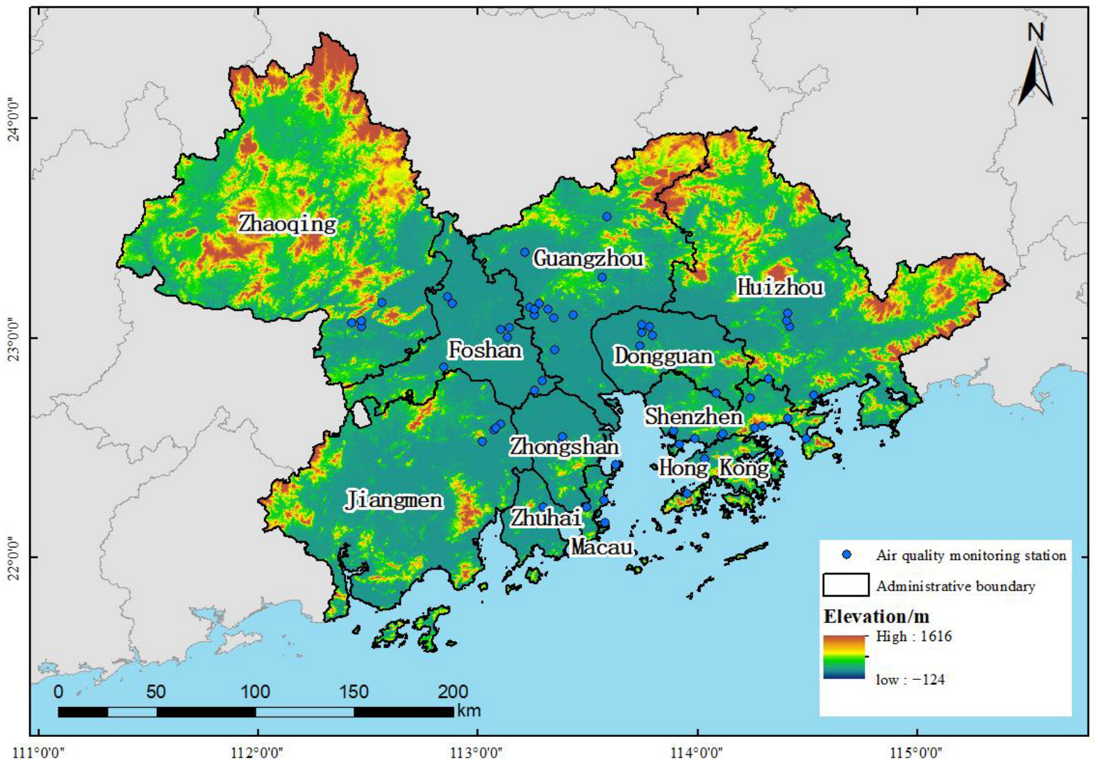
The O3 hourly concentration monitoring data for mainland China were obtained from the Urban Air Pollution Monitoring Network (https://quotsoft.net/air/, accessed on 10 November 2021) established by the China National Environmental Monitoring Center. Additionally, the monthly O3 concentration data for stations in Hong Kong and Macau were derived from the regional air monitoring network of Guangdong, Hong Kong, and Macao in the Pearl River Delta. The daily average O3 concentration was obtained by averaging the 24 h O3 concentrations. Since there are different degrees of missing O3 h in each month, the days with less than 12 h of missing concentration were excluded, and the daily average O3 concentrations of the remaining effective days were averaged to obtain the monthly average O3 concentration. The distribution of the 61 monitoring stations in the GBA is shown in Figure 1.
The Chinese high-resolution air pollution reanalysis dataset [42] was provided by the Institute of Atmospheric Physics. The dataset had a high temporal and spatial resolution, the latter reaching 15 km [43]. In this study, we used the monthly O3 data derived from the atmospheric reanalysis dataset for the period between January and December 2017. The data were processed and displayed in ArcGIS with a spatial resolution of 0.17° (approximately 20 km), which met other data resolution sizes in this paper. To obtain O3 data with spatial continuity and high accuracy, we used monitoring data to fuse the data. The details for the method can be found in Section 2.3.1.

2.2.2. Emission Inventory Data

The anthropogenic emission variables were obtained from the Chinese Multi-scale Emission Inventory Model (MEIC, http://meicmodel.org/, accessed on 10 November 2021) developed at Tsinghua University. The resolution of the inventory data is 0.25° × 0.25°. In this study, the 2017 emission inventory was selected, which included 10 emissions from 5 sectors, including NMVOC, SO2, PM2.5, PM10, organic carbon (OC), NOx, NH3, CO2, CO, black carbon (BC), etc., from transportation, residential, electricity, industry, and agriculture.

2.2.3. Atmospheric Reanalysis Dataset

In this study, the ERA-5 assimilation analysis dataset, of the European Center for Medium-Range Weather Forecast (ECMWF, https://www.ecmwf.int/en/forecasts/datasets, accessed on 10 November 2021), was selected, with a resolution of 0.25° × 0.25°.
The temperature at 2 m (T, °C), wind speed at 10 m (WS, m s−1), relative humidity (RH, %), ground pressure (PS, hPa), and total precipitation (TP, mm) were selected as the meteorological variables. Since the dataset showed that the number of sunshine hours in the study area was the same, the index of sunshine hours was excluded. As ERA-5 does not include relative humidity data, this parameter was calculated using Equation (1), on the basis of the provided dew point and surface temperature values at 2 m above the surface [44]:
R H = e 17.625 × T d c 243.04 + T d c e 17.625 × T c 243.04 + T c × 100 %
where T d c is the dew point temperature (°C), T c is the actual temperature (°C), and RH is the relative humidity (%).

2.2.4. Land Cover

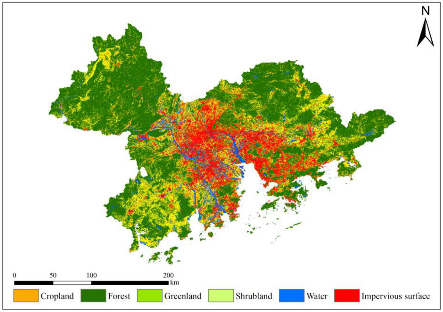
The land cover data were obtained from the 2017 global land cover dataset (FROM-GLC30) collected by Tsinghua University, with a resolution of 30 m. After strict verification, the data accuracy was estimated at 72.35% [45]. The land cover types that characterize the GBA include cropland, forest, grassland, shrubland, wetland, water, impervious surface, and bare land. The detail is shown in Figure 2.

2.3. Methods

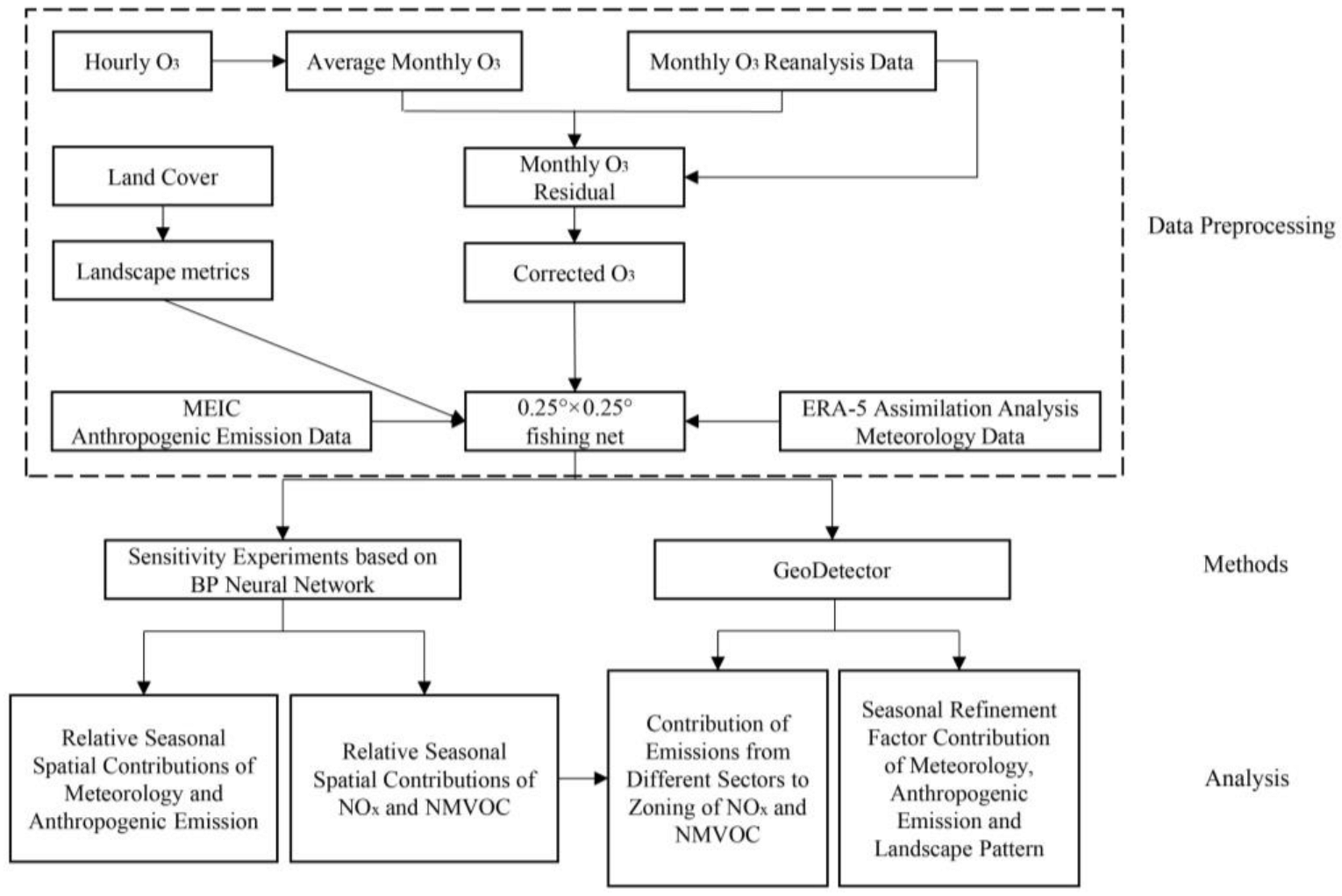
The flow chart of the study is shown in Figure 3. Firstly, the data was pre-processed. Secondly, sensitivity experiments on the basis of the BP network were performed to calculate the spatial distribution of the contribution of meteorological and emission factors to O3, and then the GeoDetector model was used to refine the contribution of meteorology, emission, and landscape variables to regional O3.

2.3.1. Data Fusion

Since the monitoring stations of air pollution reanalysis data did not include some areas of Hong Kong and Macao [43], the data of monitoring stations were used to correct the air pollution data for the GBA. The specific steps are as follows [46]. First, the monthly monitoring station data values were subtracted from the O3 reanalysis data values to calculate the monthly concentration residuals at the monitoring locations, then ordinary kriging interpolation was performed on the concentration residuals to generate a 0.17° × 0.17° monthly concentration residual map. Finally, the monthly residual interpolation values were added to the reanalysis data grid to obtain the corrected monthly concentrations for each grid. The calculation equation is as follows.
r i = m i a i
C ^ j = a j r ^ j
where r i is the monthly concentration residual of monitoring point i , m i is the monthly monitoring data of monitoring point i , a i is the monthly O3 reanalysis value on the grid corresponding to monitoring point i , a j represents the monthly O3 reanalysis value on grid j , r ^ j is the monthly residual after interpolation on grid j , and C ^ j represents the monthly corrected O3 on grid j .

2.3.2. Landscape Metrics

Landscape metrics highly condense the information on landscape patterns, effectively reflecting the composition and spatial configuration of the landscape structure. In this study, several landscape metrics were selected to quantify the landscape pattern in the GBA. Table 1 describes in detail the selected landscape indicators, which were: landscape area (LPI), landscape shape (LSI, SHAPE_MN), landscape diversity (SHDI, CONTAG), and landscape agglomeration (AI).

2.3.3. Sensitivity Analysis of Contribution

  • BP neural network model
A two-layer BP neural network was used for the simulations. The number ratio of the input layer, hidden layer, and output layer was 1:1:1. The tangent log sigmoid function was selected as the transfer function of the hidden layer, and the linear function was the transfer function of the output layer.
The input layer neurons were meteorological variables, emission variables, and landscape pattern variables. The number of neurons in the hidden layer was tested with 19 hidden layers and 5 neurons. The learning rate was set to 0.05 and the target error to 0.0001 for simulation. The BP network was trained using 119 rasters corresponding to January to December 2017 data from the study area (1428 in total). The model performance was evaluated using a tenfold cross-test, which divides all data into ten sub-samples, retaining one sub-sample each time as validation data, and the remaining nine sub-samples were used for model training. The process was repeated ten times to obtain R2 and root mean square error (RSME) as indicators for evaluating model performance.
2.
Experimental design and analysis
Four experiments (Table 2) were designed to simulate O3 concentration at specific x (base time) and y (aim time) times [28]. The contributions of meteorology (NOx) (EXPy,x) and emission (NMVOC) (EXPx,y) to O3 concentration were quantified using the O3 concentration simulated by different combinations of the same variables at x and y times. The simulated concentrations of x and y time were compared through a linear relationship to evaluate the contribution of meteorology (NOx) and emission (NMVOC) to the change in O3 concentration. The normalization contribution was then calculated. The formulas adopted are shown in Equations (4)–(7).
C o n M e t / N O x = O 3 E X P x , x O 3 E X P y , x O 3 E X P x , x O 3 E X P y , y
C o n E m i / N M V O C = O 3 E X P x , x O 3 E X P x , y O 3 E X P x , x O 3 E X P y , y
N C o n M e t / N O x = C o n M e t / N O x C o n M e t / N O x + C o n E m i / N M V O C
N C o n E m i / N M V O C = Con Emi / N M V O C Con Met / N O x + Con Emi / N M V O C
O3 E X P x , x ,, O3 E X P y , y , O3 E X P y , x and O3 E X P x , y , respectively, represent the O3 concentrations simulated by E X P x , x , E X P y , y , E X P y , x , and E X P x , y ; C o n M e t / N O x and C o n E m i / N M V O C represent the contributions of meteorology and emission (NOx and NMVOC), respectively; and N C o n M e t / N O x and N C o n E m i / N M V O C represent the normalized contributions of meteorology and emission (NOx and NMVOC), respectively.
3.
Analysis of sensitivity results and selection of base time
Four cases exist for the results obtained from C o n M e t and C o n E m i calculated by Equations (4) and (5), respectively (Table 3).
After statistical analyses, the grids with the lowest monthly O3 concentration were selected as the base time y input models to make comparisons with other seasons.

2.3.4. Geode Ector

The GeoDetector software comprises a set of statistical methods that can detect spatial differentiation and reveal potential driving forces. Models can be performed to assess nonlinear relationships between potential factors and target geographic phenomena. The core idea at the base of the model assumption is that if an independent variable has an important influence on a dependent variable, then the spatial distribution of the two variables should be similar [47].
The spatial correlation of X (e.g., meteorological variables, anthropogenic emission variables, and landscape pattern variables) and Y (e.g., ground-level O3 concentration) can be measured by q statistics, which are defined as:
q = 1 h = 1 L N h σ h N σ h = 1 S S W S S T  
S S W = h = 1 L N h σ h
S S T = N σ h
where h = 1, …, L is the category of factor X, and Nh and N are the h category and sample size of the entire study area, respectively. SSW and SST are the sum of variance and total variance, respectively, of the h category and the entire study area. The value of q is [0, 1]. The greater the value of q, the higher the correlation with O3. The effect of the interaction between two X variables on O3 can also be quantified by q statistics.

3. Results

3.1. O3 Concentration Temporal and Spatial Differentiation Characteristics

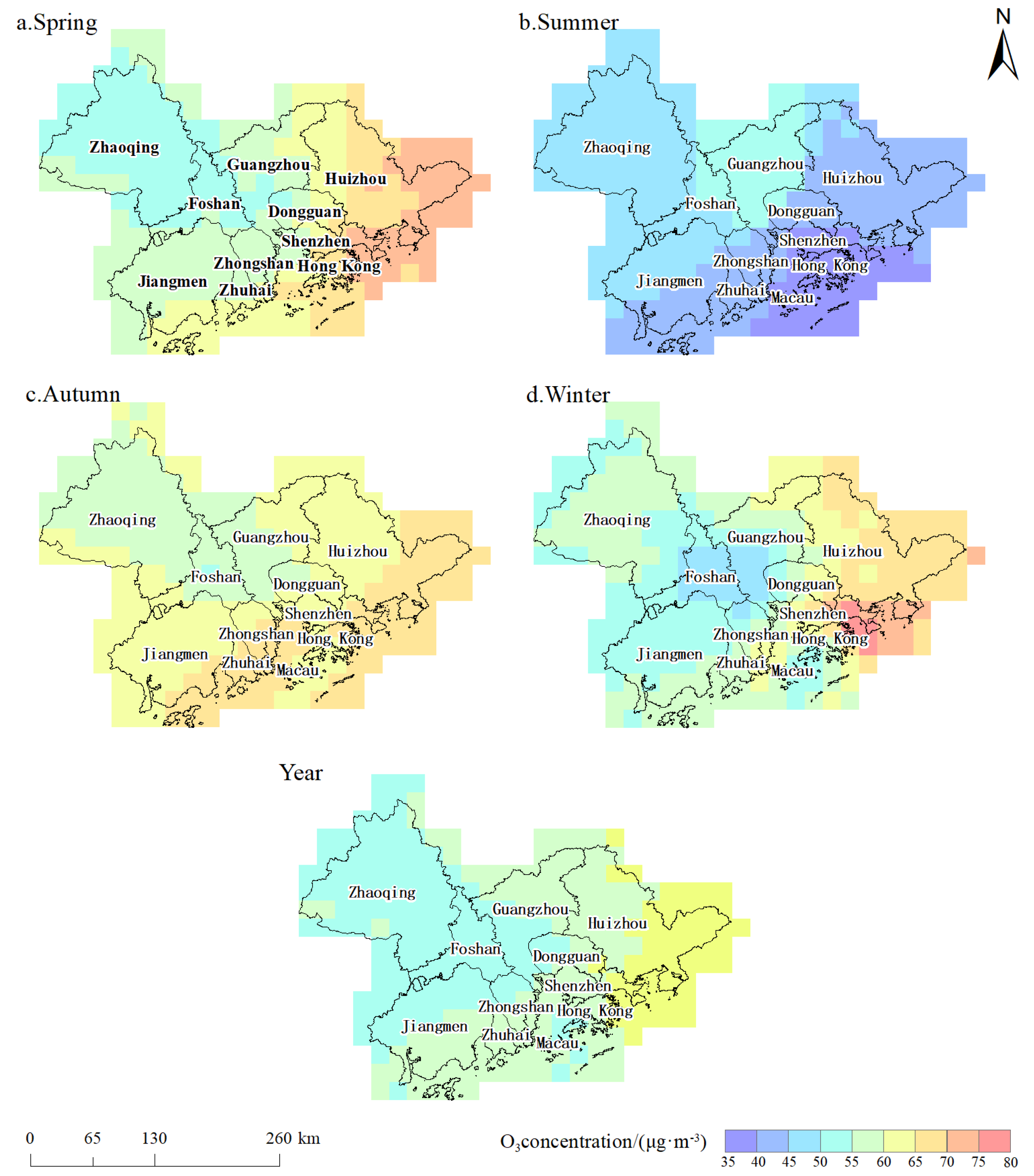
The corrected O3 concentration value was verified by the monitoring data (Appendix A). The mean annual and seasonal O3 distribution in the GBA for the year 2017 is shown in Figure 4. Based on the mean annual data, the areas with high O3 concentrations were in the southeast of the GBA, specifically, southeast of Huizhou. The low-concentration areas were located in the northwest cities, such as Zhaoqing, Foshan, and part of Guangzhou, Jiangmen, and Hong Kong. Based on the mean seasonal data (a–d), O3 concentration was the lowest in summer (mean 44.6 μg/m3), followed by winter (mean 60 μg/m3), spring (mean 60.2 μg/m3), and was the highest in autumn (mean 62.8 μg/m3). The spatial distribution of O3 in the GBA was different between seasons: it was similar in spring, autumn, and winter when O3 concentration was low in the northwest and high in the southeast, while it was different in summer, with low O3 concentrations in the southeast, and high concentrations in the central areas.

3.2. Sensitivity Experiments Results

3.2.1. Model Accuracy Verification

The BP network training results are shown in Table 4. The model reached the training goal after being trained 20 times, obtaining a total simulated decision coefficient ( R 2 ) of 0.89. The coefficient of determination of seasons ranged from 0.4 to 0.8, and the simulation accuracy was poor in summer and winter. The decadal crossover results showed R CV 2 of 0.67 and RMSE of 7.53, and the model simulation accuracy was good.

3.2.2. Relative Contribution of Seasonal Meteorology and Emissions to O3 Variation

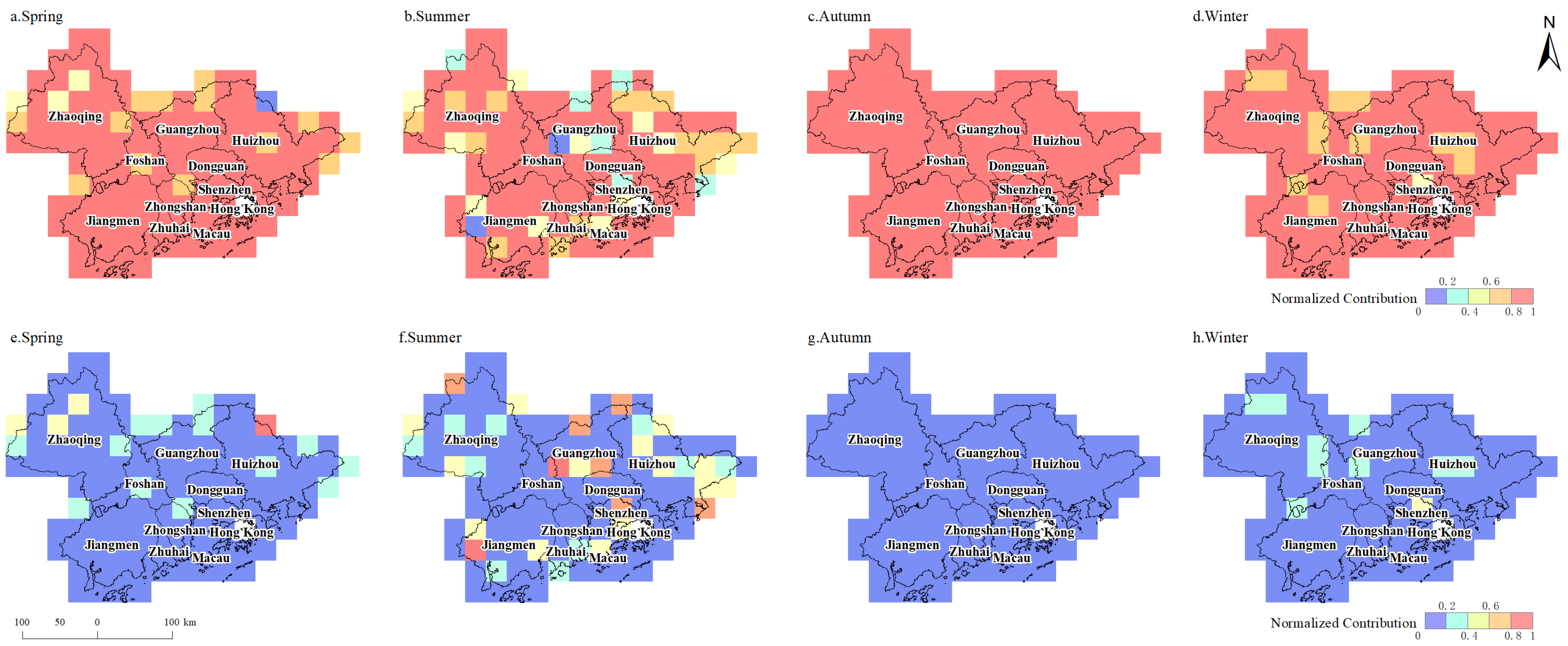
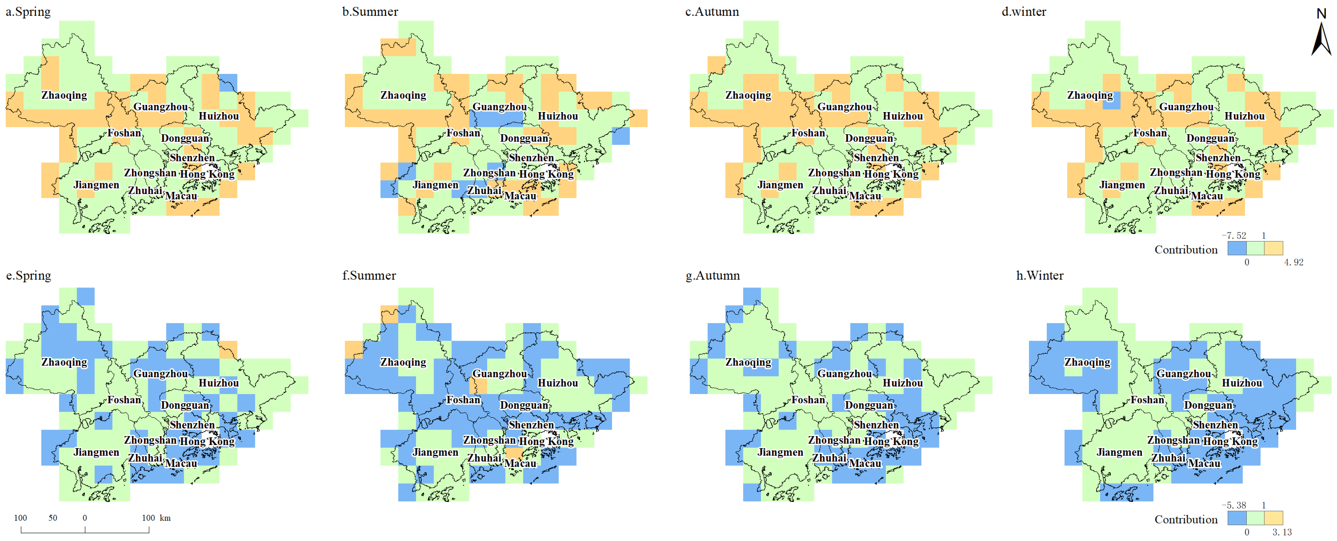
Figure 5 shows the normalized contributions of meteorological factors and emissions for the four seasons obtained from the neural network simulation. The GBA was dominated by meteorological factors, the emission contribution was weak, and the distribution of normalized contribution size varied among the four seasons. The normalized contributions in spring, summer, and winter were similar, and the overall contribution of meteorological conditions to O3 accounted for more than 60%. O3 was most influenced by meteorological conditions in autumn. In summer, O3 in the GBA was controlled mainly by meteorological conditions, and the meteorological factors normalized contribution decreased relative to other seasons, while the contribution of emissions was relatively higher. In spring, Jiangmen, Zhuhai, Zhongshan, Dongguan, Shenzhen, and Macao were relatively strongly controlled by meteorological factors, with the normalized contribution reaching more than 80%, while Zhaoqing, Foshan, Guangzhou, and Huizhou were relatively weakly controlled by meteorology, with the contribution of emissions ranging from 0 to 60%. In summer, Zhongshan and Foshan were subject to relatively high intensity of meteorological factors control, while Huizhou, Shenzhen, Hong Kong, Zhuhai, and Guangzhou were subject to relatively low intensity of meteorological factors control, with normalized contributions ranging from 0% to 60%. In the autumn, the overall contribution of meteorological factors to O3 in the GBA reached more than 80%. In winter, except for central Huizhou, part of Guangzhou, Zhaoqing, Shenzhen, and other areas suffered from the role of emissions of 20% to 60%, and other areas suffered from the role of meteorological factors of more than 80%.
Figure 6 shows the contributions of meteorological factors and emissions obtained from sensitivity experimental simulations, and the direction of the meteorological, and emission contributions to O3 can be inferred from the corresponding range of values (whether greater than 1) in Table 3. Regarding the meteorological factors, the meteorological factors in the GBA mainly show a facilitative effect on the production or accumulation of O3 (Con(Emi) range was dominated by less than 1, corresponding to IV in Table 3). Regarding the emission factors, the four seasonal distributions of emission directions of action were relatively stable in the GBA. Compared with the baseline conditions, the emission conditions in Foshan, central Jiangmen, southern Zhaoqing, northern Guangzhou, and central Huizhou were unfavorable for the generation of O3. Emission conditions in Zhongshan, southern Guangzhou, Zhuhai, central Zhaoqing, western Dongguan, and Jiangmen, except for the central part of the region, promoted the generation of O3 (Con(Met) range is greater than 1 is dominant, corresponding to II in Table 3). The emission conditions in Shenzhen and Macau were not conducive to O3 generation in spring, autumn, and winter, and showed a promotional effect in summer.

3.2.3. Relative Contribution of Seasonal NOx and NMVOC to O3 Variation

The sensitivity simulation results of NOx and NMVOC show (Figure 7) that the degree of contribution of NOx and NMVOC varied greatly in different seasons. In terms of the relative contribution of NOx and NMVOC, the overall O3 concentration in the GBA in spring was influenced by NMVOC, with the NCon(NMVOC) reaching more than 60% in southern Zhaoqing, southern Foshan, Dongguan, northern Jiangmen, and south-central Huizhou, and more than 60% in coastal areas such as eastern Huizhou, Zhuhai, Macao, and Hong Kong. The impact of NOx emissions on O3 concentrations in the GBA was greater in summer, with Zhaoqing, Huizhou, Macau, Hong Kong, western Jiangmen, northern Guangzhou, southern Zhongshan, western Foshan, Shenzhen, and eastern Dongguan having more than 60% of NCon(NOx), while Zhuhai was influenced mainly by NMVOC. In autumn, O3 generation in the Greater Bay Area was influenced by NMVOC, and NCon (NMVOC) reached more than 60% in most areas of Zhaoqing, Foshan, Huizhou, Zhongshan, central Jiangmen, and eastern Dongguan. O3 in the northern end of Zhaoqing, eastern Foshan, and eastern Jiangmen were influenced mainly by NOx emissions, and the relative contribution of NOx and NMVOC in the rest of the region was not significant. In winter, the southeastern part of the GBA O3 was affected mainly by NOx emissions, with Zhuhai, Dongguan, Shenzhen, Hong Kong, Macau, Guangzhou, southern and northern Huizhou, and central Foshan being more obvious, while the northwestern was affected mainly by NMVOC, with Zhaoqing as the representative.

3.3. GeoDetector Results

3.3.1. Analysis of the Factors Driving O3 Concentration

Factor detectors were used to detect the contribution of 2017 and four-season drivers to O3 concentrations (Table 5). The significant effects on O3 were due almost solely to the meteorological factors, and the significant effect of meteorological factors on O3 varied from season to season. Throughout the year, the most significant contributions to O3 were T and TP, with q values of 0.35 and 0.31, respectively, followed by RH and WS, with q values of 0.18 and 0.12, respectively, and SP, with the least contribution of 0.06. In spring, the meteorological effects on O3 were reflected mainly in T (q = 0.62), WS (q = 0.35), and TP (q = 0.17), and their p-values were also less than 0.01. The related directions of action showed that high temperature, low wind speed, and more precipitation in spring were the main reasons for promoting O3 formation. In summer, the meteorological effect on O3 was reflected mainly in TP (q = 0.41) and RH (q = 0.21), which also showed an opposite effect with O3 concentration, indicating that more precipitation and higher humidity in summer were the reasons for inhibiting O3 formation. In addition, LSI also showed a significant effect at the 0.05 level (q = 0.11), showing that the more complex the landscape type, the more it suppressed the concentration of summer O3. In autumn, the meteorological factors, which were mainly in T (q = 0.68), had a more significant effect on O3 concentration, and showed a homogeneous effect with O3 concentration, indicating that the higher temperature in autumn in the GBA was responsible for the formation of O3. In winter, O3 concentration was controlled mainly by RH (q = 0.14) and SP (q = 0.17), suggesting that higher humidity and lower air pressure in winter were not conducive to ozone production. In addition, the landscape pattern factor CONTAG (q = 0.09) was also related to O3 concentration, showing that the aggregation of different types of patches was not conducive to higher O3 concentration in winter.

3.3.2. Interaction of Factors Affecting O3 Concentration

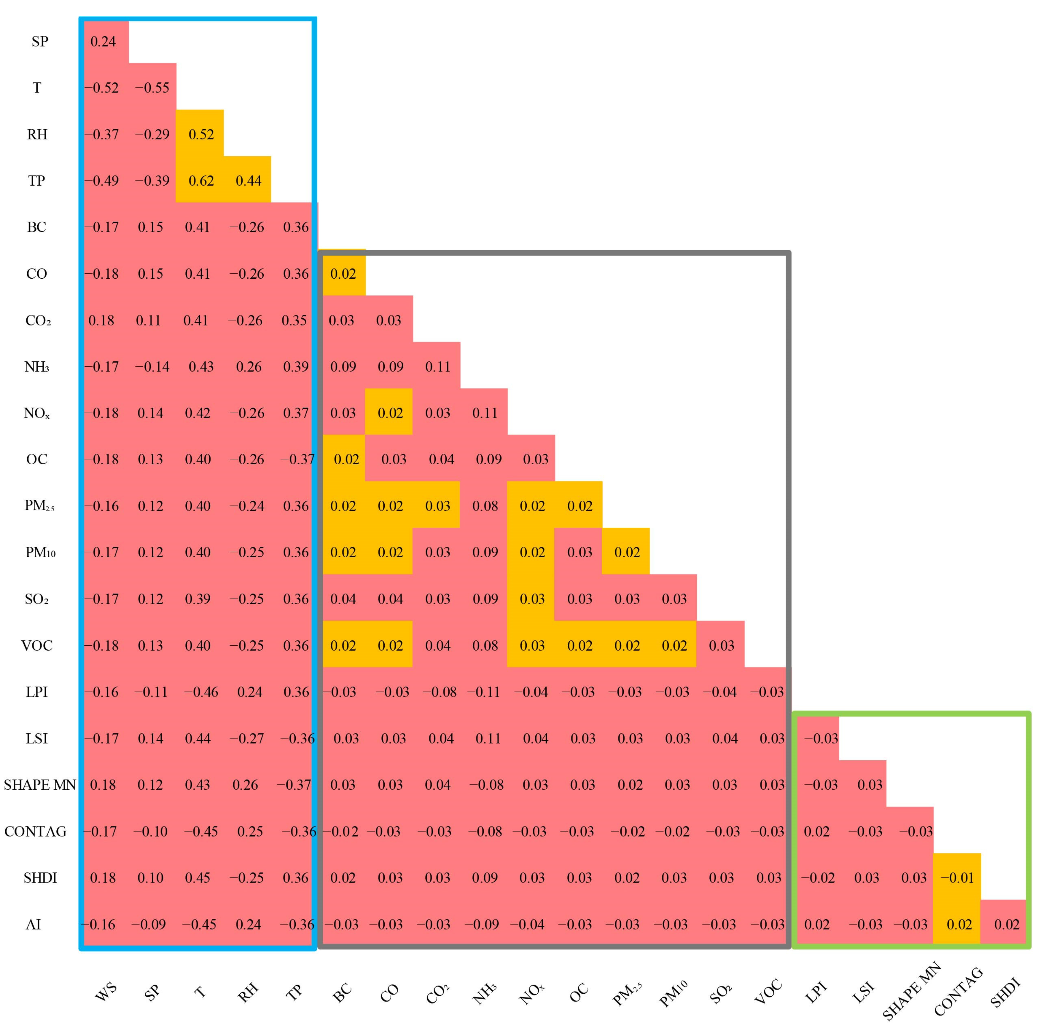
The ecological detector shows whether the two factors interacted with each other on the variation of O3 concentration. The results showed that the meteorological factors WS, T, RH, and TP interacted with anthropogenic emissions and landscape patterns to influence the O3 concentration (Table A1). The interaction detector shows the strength of the interaction between the two factors on the O3 concentration (Figure 8). It was evident that most of the factors showed a non-linear enhancement of O3 concentration between the two, i.e., the interaction between the two factors had a greater effect on the O3 concentration than the sum of the effects of the two factors alone. The interactions between meteorological factors and emission factors and landscape pattern factors were strong, with the strongest influence of the interaction between T and other factors, followed by TP and RH, and the least influence of the interaction between WS and SP and other factors.
Landscape patterns can alter local microclimate conditions. Combining Table 5 and Figure 8, it can be seen that the correlation direction of landscape pattern factors with O3 and with T were the same, and the correlation direction of T with O3 were also the same, while the correlation direction of landscape pattern factors O3 and with RH were opposite, and the correlation direction of RH with O3 was also opposite. It could be shown that the smaller the area of individual patches within the landscape pattern, the more complex the individual patch types, the lower the degree of aggregation of different patch types, and the higher the complexity and lower the aggregation of the overall landscape pattern formed, and there would be a non-linear interaction with the meteorological conditions of high temperature, high pressure, and low humidity, thus promoting the generation of O3. LSI and SHAPE MN in landscape patterns interacted in different directions with TP and WS and with O3.

3.3.3. Detection of Emission Factors Affecting Seasonal NOx and NMVOC Contributions

Factor detection of pollutant emission sector factors affecting the formation of NOx and NMVOC contributing areas in different seasons was carried out (Table 6). The change in contribution was most sensitive mainly to the residential sector, followed by NH3 emissions from the agricultural sector. The normalized contributions of NOx and NMVOC in spring were influenced mainly by BC (q = 0.38), CO (q = 0.34), CO2 (q = 0.27), NH3 (q = 0.39), NOx (q = 0.34), OC (q = 0.34), PM2.5 (q = 0.34), PM10 (q = 0.33), and NMVOC (q = 0.3) emissions from the residential sector and also by CO2 (q = 0.23) in the residential sector and NH3 (q = 0.3) emissions in the agricultural sector. Only the q value of OC passed the significance test for the sectoral anthropogenic emission contribution partition in summer. In autumn, it was affected mainly by NOx (q = 0.2), OC (q = 0.34), PM2.5 (q = 0.34), PM10 (q = 0.33), and NMVOC (q = 0.3) in the residential sector. The NOx and NMVOC contribution zoning affecting winter was similar to that of spring, but winter was not significantly affected by CO2 and NH3 emissions from the residential sector.

4. Discussion

This paper first designed four sets of sensitivity experiments based on neural networks to explore the relative contributions of meteorological factors and anthropogenic emissions in four seasons. The results show that O3 concentrations in the GBA were controlled mainly by meteorological factors, and the normalized contribution of meteorological factors reached more than 60% in all four seasons. Due to the GBA’s location in the southern coastal region of China, changes in monsoon clouds might also lead to strong seasonality in ozone concentrations [48], and the meteorological influence on O3 variability in the Bay Area was greater than in other regions [13]. Although the contribution of anthropogenic emission to the change in O3 concentrations in the GBA during all seasons was relatively small, it was the main driver of the long-term upward trend in O3 concentrations [49]. This paper also refined the spatial distribution of the direction of the contribution of meteorological and anthropogenic emission factors to O3 production. The results show that meteorology in the four seasons had a major role in promoting O3 concentrations in the GBA, and the distribution of emission factor on the production or accumulation of O3 concentrations was more stable in the four seasons in the region of promotion and mitigation, and different emission measures should be considered for the two regions.
This article quantified the effects of small factors of meteorology, anthropogenic emission, and landscape pattern on O3 concentrations, and the results showed that only meteorological factors had a significant effect on O3 at the 0.01 level. Spring O3 concentrations were related to wind speed, air temperature, and precipitation. Low wind and high-pressure stable atmospheric conditions limited convective mixing and ozone diffusion, and the weather pattern of increasing spring temperature was more conducive to accelerated O3 production [50]. In addition, precursors from biomass emissions in the Indo–Burma region of the Southeast Asian subcontinent [51,52] and southwesterly winds at 850 hPa in spring [53] contributed to O3 production, while the encounter with cold fronts or cold eddies may produce a certain amount of precipitation. The lowest O3 concentration in the GBA in summer was related mainly to precipitation and humidity, and the presence of frequent typhoon storms and plum rains in summer brought clean ocean air, diluting high O3 concentrations [16,54]. O3 concentrations were highest in the GBA in autumn, and the results of this paper showed a significant relationship between temperature and humidity. The PRD was vulnerable to tropical cyclones and subtropical high pressure in autumn, and the ground conditions of enhanced solar radiation, higher temperatures, reduced cloudiness, and lower relative humidity were conducive to the photochemical reaction of O3 [55]. Meanwhile, the stable atmospheric structure of the PRD at the periphery of typhoons was also conducive to the accumulation of O3 [56]. In winter, the results showed a significant correlation between humidity and barometric pressure. In winter, northern winds prevailed in the GBA, dominated by the East Asian monsoon and influenced by the cold high pressure from the north, the humidity was lower in the GBA, and the temperature and radiation were also lower, which was not conducive to the photochemical reaction of O3 [57], while the northern wind also brought in PM2.5 pollutants, and the dimming effect of aerosols further inhibited the production of O3 [58]. In addition, low O3 air masses from the equatorial tropical low convergence zone transported by the East Asian local Hadley circulation can also reduce O3 concentrations in areas such as Hong Kong [51].
Although the direct effect of urban landscape patterns on O3 concentration was not very obvious, the results of the interaction detector showed that landscape pattern can interact with meteorological factors in a nonlinearly enhanced way to influence O3 concentration changes. The smaller the area of individual patches, the more complex individual shape, the more complex the overall landscape shape, and the lower the degree of aggregation that would interact with the ground meteorological conditions favoring O3 generation, such as high temperature, high pressure, and low humidity to promote O3 generation., Thus, increasing the area utilized by individual site types, reducing the complexity of individual site shapes, and increasing the aggregation of different site types can suppress the generation of O3. Additionally, these landscape pattern changes that favor O3 formation also correspond to the development of urbanization [59]. It had been shown that the evolution of the urban heat island effect and changes in the thermal cycle caused by changes in urban structure due to urbanization and heat generated by anthropogenic heat sources can affect O3 concentration [54,60,61,62,63]. Mitigating O3 concentrations can also be achieved by introducing new landscapes to improve local microclimates. Studies have shown that the Wind-Corridor project can indirectly change meteorological factors, such as humidity, insolation, and evaporation by introducing more strong winds, thus reducing air pollution, while the project can also effectively mitigate the urban heat island effect [20,64], thereby reducing photochemical reactions. Therefore, the reduction of O3 concentration can be achieved not only by reducing industrial activities and traffic inducement but also by changing the urban landscape pattern indirectly and permanently. The results of this paper also showed that landscape pattern factors, especially the interaction of individual patch shape and overall landscape type with wind speed and precipitation, were more complex for O3 concentration.
This paper also quantified the relative contributions of NOx and NMVOC to O3 in the GBA. Compared with the NOx/VOC limit—which indicates that as NOx (VOC) concentration increases, O3 concentration increases, and as VOC (NOx) concentration increases [65], O3 concentration decreases—the relative contribution zone of NOx (VOC) represents the greater effect of the increase or decrease of unit NOx (VOC) concentration on the change of O3 concentration in the region. The spatial distribution of the contributions in the four seasons varied substantially, with the GBA dominated by NMVOC contributions in spring and autumn, NOx contributions in summer, and winter showing VOC contributions in the northwest and NOx contributions in the southeast. The results of the study are similar to the results of Hu et al., with a moderate VOC-limited state in spring and autumn and a weaker VOC-limited state in summer. While Hu et al. showed a stronger VOC-controlled state in winter [66], the results of this paper showed a greater range of NOx contribution, a possible discrepant result that may be the result of different study scales and models or may be related to different quantitative focus (degree of impact and spatial extent of impact), but our results all suggest that seasonally different NOx and VOC emission controls should be developed in GBA.
The results of this paper showed that emissions of CO, BC, NOx, OC, PM2.5, PM10, and NMVOC from the residential sector and NH3 from the agricultural sector were the main factors influencing the changes in the relative contribution areas of NOx and NMVOC. CO is one of the precursors of O3, which can generate O3 with hydrocarbons through HOx and NOx by radical catalytic reaction [55]. BC and CO may have a close source, and there was a good positive correlation between the two [67]. In addition, BC, OC, NH3, PM2.5, and PM10 as aerosols and their precursors can also influence the photochemical reaction of O3 by affecting UV radiation [68,69]. For emission sources, biomass combustion was the major source of NH3, NOx, CO, OC, and BC [70]. Biomass combustion, biogenic sources, paints/varnishes, and household solvents were also important sources of ambient VOC in the PRD region [71,72], and there was an enhancing trend of HCHO in some densely populated areas [73]. The results of this paper also emphasized the need for research on the mechanisms of O3 formation from residential sector emissions in highly urbanized and densely populated areas, such as the GBA and the Yangtze River Delta region.
Considering that the dilution effect of wind speed on O3 concentrations may have an impact in quantifying the contribution of local landscape pattern factors to O3 concentrations, we additionally conducted experiments at different levels of wind speed, but the results showed little difference, so they are not discussed here (Table A2). The limitation of this work is that, firstly, in order to remedy the problem that the assimilation data of reanalysis data lack site data in Hong Kong and Macao, this paper used monitoring data to fuse with reanalysis pollution data, and this fusion method could be influenced by the distribution of sites, and the accuracy of O3 concentration in areas with few sites may be impacted. Second, the landscape pattern of individual site types was not studied in this work. In addition, when studying the relationship between landscape patterns and environmental processes, multiple spatial scales should be selected to study or find the best study scale, but due to the limitation of data acquisition, only the highest accuracy of emissions was obtained as the scale for this paper, and further studies on this aspect will be considered in the future.
5. Conclusions

This paper studied the GBA and adopted sensitivity experiments and GeoDetector to analyze the dominant factors affecting O3 and the contribution between each factor in 2017. The main findings are as follows.
The contribution of meteorology to O3 concentration changes was dominant both in terms of region and extent, while the contribution of emissions was relatively weak, and both were dominant in contributing to O3 production. Meteorology had a significant effect on O3 concentrations. Although the direct effect of surface landscape on O3 was not obvious, it would have a nonlinear interaction with meteorological conditions to influence O3 concentration changes, and the interaction between surface landscape patterns toward urbanization and favorable meteorological conditions promoted O3 concentration generation or accumulation. Furthermore, the degree of contribution of NOx and NMVOC in the GBA varied considerably in different seasons. Residential sector emissions and agricultural sector NH3 emission were the main factors influencing the change in the relative contribution area of NOx and NMVOC, related to a large amounts of precursors from biomass burning, biogenic sources, paint/varnish, and household solvents due to the dense population in the GBA. We provide support for the development of regionally and seasonally differentiated control strategies for the mitigation of O3 concentration generation and production, as well as theoretical support for the mechanisms of urbanized surface landscape effects on O3 concentration. The impact of emissions from the residential sector on O3 sensitivity is also highlighted.

Author Contributions

Conceptualization, data curation, software, visualization, validation, writing—original draft, X.T.; methodology, validation, supervision, Y.Q.; validation, writing—review and editing, supervision, H.W.; software, validation, supervision, J.F.; conceptualization, resources, funding acquisition, J.W. All authors have read and agreed to the published version of the manuscript.

Funding

This study was funded by Shenzhen Fundamental Research Program, grant number GXWD20201231165807007-20200816003026001.

Data Availability Statement

The data in this study are open and can be made available to interested users upon contacting the corresponding author.

Conflicts of Interest

The authors declare no conflict of interest.

Appendix A

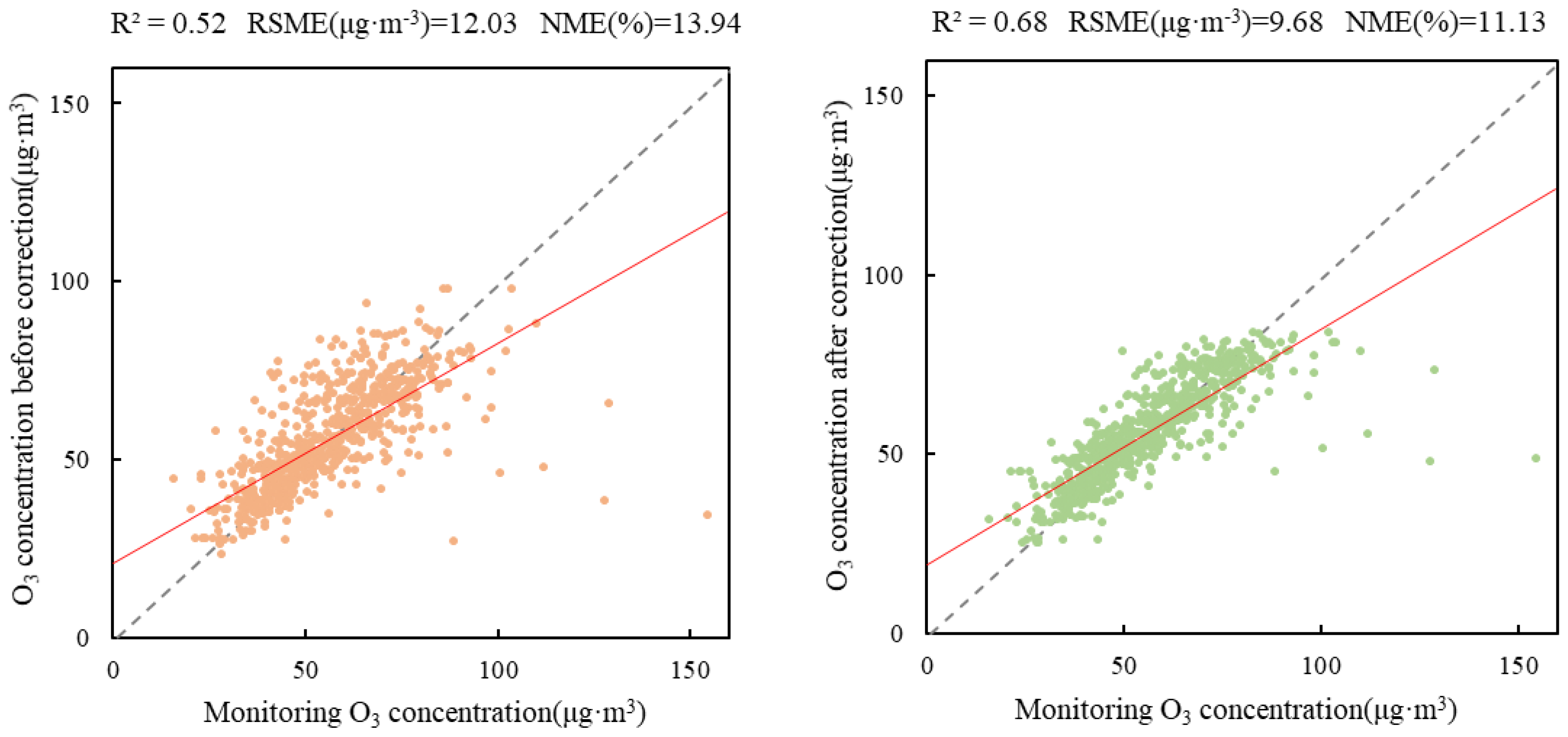
The corrected O3 was more accurate. The coefficient of determination R2 increased from 0.5 to 0.7 (Figure A1), root mean square error (RSME) decreased from 12 to 9.7, and normalized mean square error (NME) also decreased from 13.9% to 11.1%.
Figure A1. Correlation and statistical indexes between monthly O3 concentration and monthly monitored O3 concentration before and after correction.
Remotesensing 14 05796 g0a1
Table A1. Meteorology, emission, and landscape pattern ecological detection results.
WSSPTRHTPBCCOCO₂NH₃NO
SPN
TYY
RHYYY
TPYYNY
BCYNYYY
COYNYYYN
CO2YNYYYNN
NH₃YNYYYNNN
NOₓYNYYYNNNN
OCYNYYYNNNNN
PM2.5YNYYYNNNNN
PM10YNYYYNNNNN
SO₂YNYYYNNNNN
VOCYNYYYNNNNN
LPI YNYYYNNNNN
LSI YNYYYNNNNN
SHAPE MN YNYYYNNNNN
CONTAG YNYYYNNNNN
SHDI YNYYYNNNNN
AIYNYYYNNNNN
OCPM2.5PM10SO₂VOCLPILSISHAPE MNCONTAGSHDI
PM2.5N
PM10NN
SO₂NNN
VOCNNNN
LPI NNNNN
LSI NNNNNN
SHAPE MN NNNNNNN
CONTAG NNNNNNNN
SHDI NNNNNNNNN
AINNNNNNNNNN
Note: Y indicates that there is a significant difference in the effects of the two factors on O3 changes, and N means no significant difference.
Table A2. The q and p values of factor detectors for O3 concentration and landscape patterns at different wind speed classes (p-values less than 0.01 represent results significant at the 0.01 level).
WS (1–2)WS (1–2)WS (5–6)WS (7–8)WS (9–10)
qpqpqpqpqp
LPI 0.02 0.81 0.01 0.99 0.04 0.93 0.07 0.99 0.10 1.00
LSI 0.03 0.83 0.00 1.00 0.06 0.74 0.06 1.00 0.10 1.00
SHAPE MN 0.01 1.00 0.02 1.00 0.05 0.97 0.06 0.89 0.10 1.00
CONTAG 0.02 1.00 0.02 0.99 0.03 1.00 0.07 0.69 0.10 1.00
SHDI 0.02 0.98 0.03 0.70 0.05 1.00 0.04 0.97 0.08 1.00
AI0.03 1.00 0.01 1.00 0.03 1.00 0.08 0.91 0.07 1.00

References

  1. World Health Organization. Air Quality Guidelines: Global Update 2005: Particulate Matter, Ozone, Nitrogen Dioxide, and Sulfur Dioxide; World Health Organization: Geneva, Switzerland, 2006.
  2. Zhao, N.; Pinault, L.; Toyib, O.; Vanos, J.; Tjepkema, M.; Cakmak, S. Long-term ozone exposure and mortality from neurological diseases in Canada. Environ. Int. 2021, 157, 106817. [Google Scholar] [CrossRef]
  3. Mahmood, F.; Khokhar, M.F.; Mahmood, Z. Examining the relationship of tropospheric ozone and climate change on crop productivity using the multivariate panel data techniques. J. Environ. Manag. 2020, 272, 111024. [Google Scholar] [CrossRef]
  4. Maji, K.J.; Ye, W.-F.; Arora, M.; Nagendra, S.M.S. Ozone pollution in Chinese cities: Assessment of seasonal variation, health effects and economic burden. Environ. Pollut. 2019, 247, 792–801. [Google Scholar] [CrossRef] [PubMed]
  5. Ugalde-Resano, R.; Riojas-Rodríguez, H.; Texcalac-Sangrador, J.L.; Cruz, J.C.; Hurtado-Díaz, M. Short term exposure to ambient air pollutants and cardiovascular emergency department visits in Mexico city. Environ. Res. 2022, 207, 112600. [Google Scholar] [CrossRef] [PubMed]
  6. Wang, Z.-b.; Li, J.-x.; Liang, L.-w. Spatio-temporal evolution of ozone pollution and its influencing factors in the Beijing-Tianjin-Hebei Urban Agglomeration. Environ. Pollut. 2020, 256, 113419. [Google Scholar] [CrossRef] [PubMed]
  7. The 2016 Report on the State of the Ecology and Environment in China; Ministry of Ecology and Environment of People’s Republic of China: Beijing, China, 2017.
  8. The 2017 Report on the State of the Ecology and Environment in China; Ministry of Ecology and Environment of People’s Republic of China: Beijing, China, 2018.
  9. The 2018 Report on the State of the Ecology and Environment in China; Ministry of Ecology and Environment of People’s Republic of China: Beijing, China, 2019.
  10. The 2019 Report on the State of the Ecology and Environment in China; Ministry of Ecology and Environment of People’s Republic of China: Beijing, China, 2020.
  11. Silver, B.; Reddington, C.L.; Arnold, S.R.; Spracklen, D.V. Substantial changes in air pollution across China during 2015–2017. Environ. Res. Lett. 2018, 13, 114012. [Google Scholar] [CrossRef]
  12. Liu, Y.; Wang, T. Worsening urban ozone pollution in China from 2013 to 2017–Part 2: The effects of emission changes and implications for multi-pollutant control. Atmos. Chem. Phys. 2020, 20, 6323–6337. [Google Scholar] [CrossRef]
  13. Mousavinezhad, S.; Choi, Y.; Pouyaei, A.; Ghahremanloo, M.; Nelson, D.L. A comprehensive investigation of surface ozone pollution in China, 2015–2019: Separating the contributions from meteorology and precursor emissions. Atmos. Res. 2021, 257, 105599. [Google Scholar] [CrossRef]
  14. Chen, Z.; Li, R.; Chen, D.; Zhuang, Y.; Gao, B.; Yang, L.; Li, M. Understanding the causal influence of major meteorological factors on ground ozone concentrations across China. J. Clean. Prod. 2020, 242, 118498. [Google Scholar] [CrossRef]
  15. Han, H.; Liu, J.; Shu, L.; Wang, T.; Yuan, H. Local and synoptic meteorological influences on daily variability in summertime surface ozone in eastern China. Atmos. Chem. Phys. 2020, 20, 203–222. [Google Scholar] [CrossRef]
  16. Liu, P.; Song, H.; Wang, T.; Wang, F.; Li, X.; Miao, C.; Zhao, H. Effects of meteorological conditions and anthropogenic precursors on ground-level ozone concentrations in Chinese cities. Environ. Pollut. 2020, 262, 114366. [Google Scholar] [CrossRef] [PubMed]
  17. Ma, M.; Yao, G.; Guo, J.; Bai, K. Distinct spatiotemporal variation patterns of surface ozone in China due to diverse influential factors. J. Environ. Manag. 2021, 288, 112368. [Google Scholar] [CrossRef] [PubMed]
  18. Tang, G.; Wang, Y.; Li, X.; Ji, D.; Hsu, S.; Gao, X. Spatial-temporal variations in surface ozone in Northern China as observed during 2009–2010 and possible implications for future air quality control strategies. Atmos. Chem. Phys. 2012, 12, 2757–2776. [Google Scholar] [CrossRef] [Green Version]
  19. World Health Organization. WHO Global Air Quality Guidelines: Particulate Matter (PM2.5 and PM10), Ozone, Nitrogen Dioxide, Sulfur Dioxide and Carbon Monoxide; World Health Organization: Geneva, Switzerland, 2021.
  20. Chen, Z.; Zhuang, Y.; Xie, X.; Chen, D.; Cheng, N.; Yang, L.; Li, R. Understanding long-term variations of meteorological influences on ground ozone concentrations in Beijing During 2006–2016. Environ. Pollut. 2019, 245, 29–37. [Google Scholar] [CrossRef]
  21. Fu, Y.; Tai, A.P.K. Impact of climate and land cover changes on tropospheric ozone air quality and public health in East Asia between 1980 and 2010. Atmos. Chem. Phys. 2015, 15, 10093–10106. [Google Scholar] [CrossRef] [Green Version]
  22. Lu, D.; Xu, J.; Yue, W.; Mao, W.; Yang, D.; Wang, J. Response of PM2.5 pollution to land use in China. J. Clean. Prod. 2020, 244, 118741. [Google Scholar]
  23. Tu, M.; Liu, Z.; He, C.; Fang, Z.; Lu, W. The relationships between urban landscape patterns and fine particulate pollution in China: A multiscale investigation using a geographically weighted regression model. J. Clean. Prod. 2019, 237, 117744. [Google Scholar] [CrossRef]
  24. Yang, H.; Chen, W.; Liang, Z. Impact of land use on PM2.5 pollution in a representative city of middle China. Int. J. Environ. Res. Public Health 2017, 14, 462. [Google Scholar]
  25. Cheng, J.; Su, J.; Cui, T.; Li, X.; Dong, X.; Sun, F.; Yang, Y.; Tong, D.; Zheng, Y.; Li, Y. Dominant role of emission reduction in PM2.5 air quality improvement in Beijing during 2013–2017: A model-based decomposition analysis. Atmos. Chem. Phys. 2019, 19, 6125–6146. [Google Scholar] [CrossRef] [Green Version]
  26. Li, K.; Jacob, D.J.; Liao, H.; Zhu, J.; Shah, V.; Shen, L.; Bates, K.H.; Zhang, Q.; Zhai, S. A two-pollutant strategy for improving ozone and particulate air quality in China. Nat. Geosci. 2019, 12, 906–910. [Google Scholar] [CrossRef]
  27. Liu, T.; Gong, S.; He, J.; Yu, M.; Wang, Q.; Li, H.; Liu, W.; Zhang, J.; Li, L.; Wang, X. Attributions of meteorological and emission factors to the 2015 winter severe haze pollution episodes in China’s Jing-Jin-Ji area. Atmos. Chem. Phys. 2017, 17, 2971–2980. [Google Scholar] [CrossRef] [Green Version]
  28. Zhang, W.; Wang, H.; Zhang, X.; Peng, Y.; Zhong, J.; Wang, Y.; Zhao, Y. Evaluating the contributions of changed meteorological conditions and emission to substantial reductions of PM2.5 concentration from winter 2016 to 2017 in Central and Eastern China. Sci. Total Environ. 2020, 716, 136892. [Google Scholar] [PubMed]
  29. AlOmar, M.K.; Hameed, M.M.; AlSaadi, M.A. Multi hours ahead prediction of surface ozone gas concentration: Robust artificial intelligence approach. Atmos. Pollut. Res. 2020, 11, 1572–1587. [Google Scholar] [CrossRef]
  30. Su, X.; An, J.; Zhang, Y.; Zhu, P.; Zhu, B. Prediction of ozone hourly concentrations by support vector machine and kernel extreme learning machine using wavelet transformation and partial least squares methods. Atmos. Pollut. Res. 2020, 11, 51–60. [Google Scholar] [CrossRef]
  31. Otero, N.; Sillmann, J.; Schnell, J.L.; Rust, H.W.; Butler, T. Synoptic and meteorological drivers of extreme ozone concentrations over Europe. Environ. Res. Lett. 2016, 11, 024005. [Google Scholar] [CrossRef]
  32. Sharma, A.; Mandal, T.K.; Sharma, S.K.; Shukla, D.K.; Singh, S. Relationships of surface ozone with its precursors, particulate matter and meteorology over Delhi. J. Atmos. Chem. 2017, 74, 451–474. [Google Scholar] [CrossRef]
  33. Zhao, W.; Fan, S.; Guo, H.; Gao, B.; Sun, J.; Chen, L. Assessing the impact of local meteorological variables on surface ozone in Hong Kong during 2000–2015 using quantile and multiple line regression models. Atmos. Environ. 2016, 144, 182–193. [Google Scholar] [CrossRef]
  34. Cheng, N.; Li, R.; Xu, C.; Chen, Z.; Chen, D.; Meng, F.; Cheng, B.; Ma, Z.; Zhuang, Y.; He, B. Ground ozone variations at an urban and a rural station in Beijing from 2006 to 2017: Trend, meteorological influences and formation regimes. J. Clean. Prod. 2019, 235, 11–20. [Google Scholar] [CrossRef]
  35. Chen, Y.; Yan, H.; Yao, Y.; Zeng, C.; Gao, P.; Zhuang, L.; Fan, L.; Ye, D. Relationships of ozone formation sensitivity with precursors emissions, meteorology and land use types, in Guangdong-Hong Kong-Macao Greater Bay Area, China. J. Environ. Sci. 2020, 94, 1–13. [Google Scholar] [CrossRef]
  36. Camalier, L.; Cox, W.; Dolwick, P. The effects of meteorology on ozone in urban areas and their use in assessing ozone trends. Atmos. Environ. 2007, 41, 7127–7137. [Google Scholar] [CrossRef]
  37. Taylan, O. Modelling and analysis of ozone concentration by artificial intelligent techniques for estimating air quality. Atmos. Environ. 2017, 150, 356–365. [Google Scholar] [CrossRef]
  38. Zhang, Y.H.; Su, H.; Zhong, L.J.; Cheng, Y.F.; Zeng, L.M.; Wang, X.S.; Xiang, Y.R.; Wang, J.L.; Gao, D.F.; Shao, M. Regional ozone pollution and observation-based approach for analyzing ozone–precursor relationship during the PRIDE-PRD2004 campaign. Atmos. Environ. 2008, 42, 6203–6218. [Google Scholar] [CrossRef]
  39. Reddy, B.S.K.; Kumar, K.R.; Balakrishnaiah, G.; Gopal, K.R.; Reddy, R.R.; Ahammed, Y.N.; Narasimhulu, K.; Reddy, L.S.S.; Lal, S. Observational studies on the variations in surface ozone concentration at Anantapur in southern India. Atmos. Res. 2010, 98, 125–139. [Google Scholar] [CrossRef]
  40. He, B.-J.; Wang, J.; Zhu, J.; Qi, J. Beating the urban heat: Situation, background, impacts and the way forward in China. Renew. Sustain. Energy Rev. 2022, 161, 112350. [Google Scholar] [CrossRef]
  41. Guo, H.; Ling, Z.; Cheng, H.; Simpson, I.; Lyu, X.; Wang, X.; Shao, M.; Lu, H.; Ayoko, G.; Zhang, Y. Tropospheric volatile organic compounds in China. Sci. Total Environ. 2017, 574, 1021–1043. [Google Scholar] [CrossRef] [Green Version]
  42. Tang, X.; Kong, L.; Zhu, J.; Wang, Z.; Li, J.; Wu, H.; Wu, Q.; Chen, H.; Zhu, L.; Wang, W. A High-Resolution Air Quality Reanalysis Dataset over China (CAQRA); Science Data Bank: Beijing, China, 2021. [Google Scholar]
  43. Kong, L.; Tang, X.; Zhu, J.; Wang, Z.; Li, J.; Wu, H.; Wu, Q.; Chen, H.; Zhu, L.; Wang, W. A 6-year-long (2013–2018) high-resolution air quality reanalysis dataset in China based on the assimilation of surface observations from CNEMC. Earth Syst. Sci. Data 2021, 13, 529–570. [Google Scholar] [CrossRef]
  44. McNoldy, B. Temperature, Dewpoint, and Relative Humidity Calculator. Available online: http://bmcnoldy.rsmas.miami.edu/Humidity.html (accessed on 12 November 2021).
  45. Guo, Z.; Wang, C.; Liu, X.; Pang, G.; Zhu, M.; Yang, L. Accuracy assessment of the from-Glc30 land cover dataset based on watershed sampling units: A continental-scale study. Sustainability 2020, 12, 8435. [Google Scholar] [CrossRef]
  46. Liang, S.; Li, X.; Teng, Y.; Fu, H.; Chen, L.; Mao, J.; Zhang, H.; Gao, S.; Sun, Y.; Ma, Z. Estimation of health and economic benefits based on ozone exposure level with high spatial-temporal resolution by fusing satellite and station observations. Environ. Pollut. 2019, 255, 113267. [Google Scholar] [CrossRef]
  47. Wang, J.F.; Xu, C.D. Geodetector: Principle and prospective. Acta Geogr. Sin. 2017, 72, 116–134. [Google Scholar]
  48. Yin, C.; Deng, X.; Zou, Y.; Solmon, F.; Li, F.; Deng, T. Trend analysis of surface ozone at suburban Guangzhou, China. Sci. Total Environ. 2019, 695, 133880. [Google Scholar] [CrossRef]
  49. Yang, L.; Luo, H.; Yuan, Z.; Zheng, J.; Huang, Z.; Li, C.; Lin, X.; Louie, P.K.K.; Chen, D.; Bian, Y. Quantitative impacts of meteorology and precursor emission changes on the long-term trend of ambient ozone over the Pearl River Delta, China, and implications for ozone control strategy. Atmos. Chem. Phys. 2019, 19, 12901–12916. [Google Scholar] [CrossRef] [Green Version]
  50. Lee, Y.C.; Chan, K.L.; Wenig, M.O. Springtime warming and biomass burning causing ozone episodes in South and Southwest China. Air Qual. Atmos. Health 2019, 12, 919–931. [Google Scholar] [CrossRef] [Green Version]
  51. Chan, C.; Chan, L.; Chang, W.; Zheng, Y.; Cui, H.; Zheng, X.; Qin, Y.; Li, Y.S. Characteristics of a tropospheric ozone profile and implications for the origin of ozone over subtropical China in the spring of 2001. J. Geophys. Res. Atmos. 2003, 108, 8800. [Google Scholar] [CrossRef]
  52. Chan, C.Y.; Chan, L.Y.; Harris, J.M.; Oltmans, S.J.; Blake, D.R.; Qin, Y.; Zheng, Y.G.; Zheng, X.D. Characteristics of biomass burning emission sources, transport, and chemical speciation in enhanced springtime tropospheric ozone profile over Hong Kong. J. Geophys. Res. Atmos. 2003, 108, ACH3-1–ACH3-13. [Google Scholar] [CrossRef] [Green Version]
  53. Ge, C.; Liu, J.; Cheng, X.; Fang, K.; Chen, Z.; Chen, Z.; Hu, J.; Jiang, D.; Shen, L.; Yang, M. Impact of regional transport on high ozone episodes in southeast coastal regions of China. Atmos. Pollut. Res. 2022, 13, 101497. [Google Scholar] [CrossRef]
  54. Wang, Y.; Du, H.; Xu, Y.; Lu, D.; Wang, X.; Guo, Z. Temporal and spatial variation relationship and influence factors on surface urban heat island and ozone pollution in the Yangtze River Delta, China. Sci. Total Environ. 2018, 631, 921–933. [Google Scholar] [CrossRef]
  55. Ouyang, S.; Deng, T.; Liu, R.; Chen, J.; He, G.; Leung, J.C.-H.; Wang, N.; Liu, S.C. Impact of a subtropical high and a typhoon on a severe ozone pollution episode in the Pearl River Delta, China. Atmos. Chem. Phys. Discuss. 2022, 22, 10751–10767. [Google Scholar] [CrossRef]
  56. Deng, T.; Wang, T.; Wang, S.; Zou, Y.; Yin, C.; Li, F.; Liu, L.; Wang, N.; Song, L.; Wu, C. Impact of typhoon periphery on high ozone and high aerosol pollution in the Pearl River Delta region. Sci. Total Environ. 2019, 668, 617–630. [Google Scholar] [CrossRef]
  57. Gong, S.; Liu, Y.; He, J.; Zhang, L.; Lu, S.; Zhang, X. Multi-scale analysis of the impacts of meteorology and emissions on PM2.5 and O3 trends at various regions in China from 2013 to 2020 1: Synoptic circulation patterns and pollution. Sci. Total Environ. 2022, 815, 152770. [Google Scholar] [CrossRef]
  58. Zhang, X.; Xiao, X.; Wang, F.; Brasseur, G.; Chen, S.; Wang, J.; Gao, M. Observed sensitivities of PM2.5 and O3 extremes to meteorological conditions in China and implications for the future. Environ. Int. 2022, 168, 107428. [Google Scholar]
  59. Dadashpoor, H.; Azizi, P.; Moghadasi, M. Land use change, urbanization, and change in landscape pattern in a metropolitan area. Sci. Total Environ. 2019, 655, 707–719. [Google Scholar] [CrossRef]
  60. Cardelino, C.; Chameides, W. Natural hydrocarbons, urbanization, and urban ozone. J. Geophys. Res. Atmos. 1990, 95, 13971–13979. [Google Scholar] [CrossRef]
  61. Khiem, M.; Ooka, R.; Huang, H.; Hayami, H.; Yoshikado, H.; Kawamoto, Y. Analysis of the relationship between changes in meteorological conditions and the variation in summer ozone levels over the Central Kanto area. Adv. Meteorol. 2010, 2010, 349248. [Google Scholar] [CrossRef] [Green Version]
  62. Li, M.; Song, Y.; Mao, Z.; Liu, M.; Huang, X. Impacts of thermal circulations induced by urbanization on ozone formation in the Pearl River Delta region, China. Atmos. Environ. 2016, 127, 382–392. [Google Scholar] [CrossRef]
  63. Tong, N.Y.O.; Leung, D.Y.C.; Liu, C.-H. A review on ozone evolution and its relationship with boundary layer characteristics in urban environments. Water Air Soil Pollut. 2011, 214, 13–36. [Google Scholar] [CrossRef]
  64. Chen, Z.; Cai, J.; Gao, B.; Xu, B.; Dai, S.; He, B.; Xie, X. Detecting the causality influence of individual meteorological factors on local PM2.5 concentration in the Jing-Jin-Ji region. Sci. Rep. 2017, 7, 40735. [Google Scholar] [CrossRef] [Green Version]
  65. Wang, T.; Xue, L.; Brimblecombe, P.; Lam, Y.F.; Li, L.; Zhang, L. Ozone pollution in China: A review of concentrations, meteorological influences, chemical precursors, and effects. Sci. Total Environ. 2017, 575, 1582–1596. [Google Scholar] [CrossRef]
  66. Shi, B.; Yuan, X.; Zheng, C.; Yu, Y.; Huang, Z.; Zheng, J. VOC emission caps constrained by air quality targets based on response surface model: A case study in the Pearl River Delta Region, China. J. Environ. Sci. 2022; in press. [Google Scholar]
  67. Latha, K.M.; Badarinath, K.V.S. Correlation between black carbon aerosols, carbon monoxide and tropospheric ozone over a tropical urban site. Atmos. Res. 2004, 71, 265–274. [Google Scholar] [CrossRef]
  68. Gao, J.; Zhu, B.; Xiao, H.; Kang, H.; Pan, C.; Wang, D.; Wang, H. Effects of black carbon and boundary layer interaction on surface ozone in Nanjing, China. Atmos. Chem. Phys. 2018, 18, 7081–7094. [Google Scholar] [CrossRef] [Green Version]
  69. Lim, H.-J.; Turpin, B.J. Origins of primary and secondary organic aerosol in Atlanta: Results of time-resolved measurements during the Atlanta supersite experiment. Environ. Sci. Technol. 2002, 36, 4489–4496. [Google Scholar] [CrossRef]
  70. Deng, X.; Tie, X.; Zhou, X.; Wu, D.; Zhong, L.; Tan, H.; Li, F.; Huang, X.; Bi, X.; Deng, T. Effects of Southeast Asia biomass burning on aerosols and ozone concentrations over the Pearl River Delta (PRD) region. Atmos. Environ. 2008, 42, 8493–8501. [Google Scholar] [CrossRef]
  71. Cheng, H.; Guo, H.; Saunders, S.; Lam, S.; Jiang, F.; Wang, X.; Simpson, I.; Blake, D.; Louie, P.; Wang, T. Assessing photochemical ozone formation in the Pearl River Delta with a photochemical trajectory model. Atmos. Environ. 2010, 44, 4199–4208. [Google Scholar] [CrossRef] [Green Version]
  72. Guo, H.; Cheng, H.; Ling, Z.; Louie, P.; Ayoko, G. Which emission sources are responsible for the volatile organic compounds in the atmosphere of Pearl River Delta? J. Hazard. Mater. 2011, 188, 116–124. [Google Scholar] [CrossRef] [PubMed]
  73. Jin, X.; Holloway, T. Spatial and temporal variability of ozone sensitivity over China observed from the Ozone Monitoring Instrument. J. Geophys. Res. Atmos. 2015, 120, 7229–7246. [Google Scholar] [CrossRef]
Figure 1. Spatial distribution of the monitoring sites in the study area.
Remotesensing 14 05796 g001
Figure 2. Land cover types in the GBA.
Remotesensing 14 05796 g002
Figure 3. Research Flowchart.
Remotesensing 14 05796 g003
Figure 4. Average annual and seasonal distribution of O3 in the GBA in 2017. (ad) represents the four seasons.
Remotesensing 14 05796 g004
Figure 5. Distribution of the normalized contribution of seasonal meteorology and emission in the GBA. (ad) for normalized meteorological contributions and (eh) for normalized emission contributions).
Remotesensing 14 05796 g005
Figure 6. Distribution of the contribution degrees of seasonal meteorology and emission in the GBA. (ad) for meteorological contribution and (eh) for emission contribution).
Remotesensing 14 05796 g006
Figure 7. Distribution of the normalized contribution of seasonal NOx and NMVOC in the GBA. (ad) represents the four seasons.
Remotesensing 14 05796 g007
Figure 8. Strength of the interaction between meteorology, anthropogenic emission, and landscape patterns on O3 concentrations. (Red represents non-linear enhancement, and orange represents double enhancement. The negative sign represents the opposite relationship between the two factors. Blue, grey, and green represent the interaction between each factor and meteorological, emission, and landscape pattern factors, respectively).
Remotesensing 14 05796 g008
Table 1. Ecological meanings of the selected landscape metrics.
Index PropertiesIndicatorsEcological Meaning
Area and MarginLargest Plaque Area (LPI)Indicates the influence degree of the largest patch on the entire land cover type or landscape.
ShapeLandscape Shape Index (LSI)Represents the total length of the boundary (multiplied by the square correction constant) divided by the square root of the total landscape area; the larger the value, the more complex the type.
Mean Shape Index (SHAPE_MN)The patch perimeter is divided by the smallest possible perimeter of the most compact patch, reflecting the complexity of the shape of a single patch.
HeterogeneityContagion Index (CONTAG)Describes the non-randomness, or degree of agglomeration, of different patch types in the landscape.
Shannon Diversity Index (SHDI)Reflects the diversity of the landscape; the higher the value, the richer the diversity of the landscape.
AggregationAggregation Index (AI)Indicates the degree of aggregation of the landscape.
Table 2. BP network model used in the sensitivity contribution experiments.
ExperimentsDescription
E X P x , x Model run with meteorology (NOx) at x time and emissions (NMVOC) at x time
E X P y , x Model run with meteorology (NOx) at y time and emissions (NMVOC) at x time
E X P x , y Model run with meteorology (NOx) at x time and emissions (NMVOC) at y time
E X P y , y Model run with meteorology (NOx) at y time and emissions (NMVOC) at y time
Table 3. Sensitivity contribution results and corresponding meteorological conditions.
Result ValueCorresponding RangeCorresponding Results
I. C o n M e t > 1 E X P y , y > E X P y , x Compared with the baseline, emission promotes a decrease in O₃.
II. C o n M e t < 1 E X P y , y < E X P y , x or E X P x , x < E X P y , x Compared with the baseline, emission promotes an increase in O₃.
III. C o n E m i > 1 E X P y , y > E X P x , y Compared with the baseline, meteorology promotes a decrease in O₃.
IV. C o n E m i < 1 E X P y , y < E X P x , y or E X P x , x < E X P x , y Compared with the baseline, meteorology promotes an increase in O₃.
Table 4. RSME of the BP network model.
YearSpringSummerAutumnWinterCV
R20.890.810.510.780.400.63
RSME8.316.644.865.277.060.79
Table 5. The q statistics and correlation direction of the factors driving O3 concentration in the GBA. Positive and negative signs in parentheses represent the direction of the correlation.
Factors2017SpringSummerAutumnWinter
WS(+)0.12 **(−)0.35 **(−)0.11(+)0.12(+)0.11
SP(+)0.06 **(+)0.04(−)0.17(−)0.01(+)0.17 *
T(−)0.35 **(+)0.62 **(+)0.04(+)0.68 **(+)0.15
RH(−)0.180 **(−)0.08(−)0.21 *(−)0.20 **(−)0.14 **
TP(+)0.31 **(+)0.17 **(−)0.41 **(+)0.09(+)0.10
BC(+)0.01(+)0.05(−)0.04(+)0.01(+)0.08
CO(−)0.01(+)0.06(−)0.05(+)0.01(+)0.11
CO₂(+)0.01(+)0.06(−)0.05(+)0.01(+)0.11
NH₃(−)0.02(+)0.08(−)0.04(−)0.01(+)0.06
NOₓ(+)0.01(+)0.07(−)0.05(+)0.01(+)0.10
OC(+)0.01(+)0.04(−)0.03(+)0.01(+)0.05
PM₂.₅(+)0.01(+)0.06(−)0.04(+)0.01(+)0.07
PMcoarse(+)0.01(+)0.05(−)0.04(+)0.01(+)0.07
SO₂(+)0.01(+)0.05(−)0.04(+)0.01(+)0.08
NMVOC(+)0.01(+)0.06(−)0.04(+)0.02(+)0.08
LPI (−)0.01(−)0.02(+)0.07(−)0.01(−)0.08
LSI (+)0.01(+)0.05(−)0.11 *(+)0.01(+)0.14
SHAPE_MN(+)0.01(+)0.03(−)0.09(+)0.01(+)0.10
CONTAG(−)0.01(−)0.03(+)0.08(−)0.01(−)0.09 *
SHDI(+)0.01(+)0.03(−)0.09(+)0.01(+)0.09
AI(−)0.01(−)0.03(+)0.08(−)0.01(−)0.11
**. Significantly correlated at the 0.01 level (bilaterally). *. Significantly correlated at the 0.05 level (bilaterally).
Table 6. Seasonal detection results of different sectoral emissions for NCon(NOx) and NCon(NMVOC).
BCCO
SpringSummerAutumnWinterSpringSummerAutumnWinter
Transportation0.20 *0.12 0.04 0.06 0.09 0.06 0.03 0.07
Residential0.38 **0.11 0.17 0.38 **0.34 **0.07 0.14 0.39 **
Power0.14 0.07 0.06 0.10 0.14 0.12 0.08 0.10
Industry0.12 0.06 0.07 0.05 0.14 0.09 0.09 0.04
Agriculture////////
CO2NH3
SpringSummerAutumnWinterSpringSummerAutumnWinter
Transportation0.09 0.06 0.03 0.07 0.09 0.06 0.03 0.07
Residential0.27 **0.10 0.15 0.07 0.39 **0.09 0.15 0.28
Power0.15 0.10 0.08 0.06 ////
Industry0.13 0.11 0.10 0.06 ////
Agriculture////0.25 **0.10 0.14 0.27 **
NOxOC
SpringSummerAutumnWinterSpringSummerAutumnWinter
Transportation0.14 0.06 0.04 0.06 0.14 0.12 0.04 0.06
Residential0.34 **0.08 0.20 *0.34 **0.34 **0.34 **0.34 **0.34 **
Power0.11 0.11 0.07 0.11 0.11 0.11 0.11 0.11
Industry0.14 0.12 0.08 0.06 0.13 0.13 0.13 0.13
Agriculture////////
PM2.5PM10
SpringSummerAutumnWinterSpringSummerAutumnWinter
Transportation0.14 0.19 0.14 0.14 0.14 0.14 0.14 0.14
Residential0.34 **0.07 0.34 **0.34 **0.33 **0.33 **0.33 **0.33 **
Power0.11 0.09 0.11 0.11 0.12 0.12 0.12 0.12
Industry0.14 0.13 0.14 0.14 0.14 0.14 0.14 0.14
Agriculture////////
SO2NMVOC
SpringSummerAutumnWinterSpringSummerAutumnWinter
Transportation0.080.08 0.08 0.08 0.09 0.09 0.09 0.09
Residential0.090.09 0.09 0.09 0.30 **0.30 **0.30 **0.30 **
Power0.120.12 0.12 0.12 0.10 0.10 0.10 0.10
Industry0.100.10 0.10 0.10 0.15 0.15 0.15 0.15
Agriculture ////
**. Significantly correlated at the 0.01 level (bilaterally). *. Significantly correlated at the 0.05 level (bilaterally).
Publisher’s Note: MDPI stays neutral with regard to jurisdictional claims in published maps and institutional affiliations.