Long-Time Trends in Night Sky Brightness and Ageing of SQM Radiometers

Abstract

A very wide-used instrument for the measurement of the Night Sky Brightness (NSB) is the Sky Quality Meter (SQM). One of its important issues is tracking NSB for long time and connecting its variations to changes in outdoor lighting. The stability of these radiometers is fundamental; variation on the instrument behaviour could be confused with changes of the sky brightness. The SQMs of the network of the Veneto Region (Italy) and the SQM installed at La Silla (Chile) are analysed by using the twilight method considering both sunset and dawn measurements, which allows to compensate for shifts in the SQM internal clock. The slope of the observed long-term trends ranges between 29 ± 5 and 86 ± 22 mmag_SQM arcsec⁻² year⁻¹. These high values require a correction of the measurements to continue to track NSB by those instruments. The correction is presented for an Italian site, for example: raw measures show an apparent trend towards darker sky (30 ± 5 mmag_SQM arcsec⁻² year⁻¹), after the correction a clear tendency towards a brighter polluted sky appears (−21 ± 8 mmag_SQM arcsec⁻² year⁻¹), in agreement with the estimated trend of the installed luminous flux of outdoor lighting for that area.

1. Introduction

Nowadays, we are observing a continuous growth of outdoor artificial light at night (ALAN) to improve outdoor safety and better use of outdoor spaces during the night [1,2,3]. This tendency is further supported by the increase of the efficiency of white LED sources [4].

Certainly ALAN has negative consequences on the environment, animals and plants, furthermore it has adverse effects also on human health [5,6,7,8,9,10], in particular disrupting sleeping rhythms [11,12]. Increasing the sky luminance ALAN has also reduced the contrast between stars and the night sky, decreasing their visibility [13].

The problem can be addressed by dimming lights down to levels necessary for safety reasons, reducing its duration and trespass [14]. Furthermore, dark sky reserves [15] can be created for areas requiring special attentions.

Night sky brightness can be considered a quantity able to describe the impact of ALAN on the environment, therefore, monitoring its trend allows knowing whether new action on outdoor lighting systems reduces its impact or, unluckily, increases the human ecological footprint. A review of the methods and instrument used is described in [16]. The sky brightness is measured directly from land by single radiometers and by radiometers forming networks, examples are described in [17,18] or by RGB cameras, which allow measuring the spatial distribution of the sky glow and the colour of the light, two cases are presented in [19,20]. Measurements from the sky are performed by plane [21,22,23], drones and sounding balloons [24,25,26,27,28] too, they allow analysing the light polluting sources, directly. For wider areas, satellites provide upward irradiance measurements [29,30,31,32,33].

This work focuses on a very wide-spread instrument used for the measurement of Night Sky Brightness (NSB), it is the Sky Quality Meter (SQM) [34]. It is a radiance meter used to measure the sky brightness at zenith. Its bandwidth at half maximum is between 390 nm and 600 nm, with its maximum at about 520 nm. Its low cost allows composing wide networks used to monitor NSB in many places over our planet, examples are in [35,36,37,38,39,40,41,42,43]. Another similar instrument is the Telescope Encoder and Sky Sensor (TESS) [40]. It shows a wider bandwidth spanning between 400 nm and 740 nm, a peak at 550 nm and a flatter response. Both instruments usually provide their output in a logarithmic scale of magnitudes per square arcsecond (mag arcsec⁻²).

Single devices and networks composed by these kinds of instruments are often used to analyse the trend of NSB and to follow the effect of changing in outdoor lighting systems due to their managing and dimming during the night, updating of the light sources and changing of their extensions towards new areas, for example.

In performing this kind of assessment, the stability of the instruments is fundamental. Knowing that the instrument response does not change allows to attribute NSB variations to variations in light pollution, given that the atmospheric conditions did not change significantly.

Early studies that were aiming to determine long-term NSB trends surprisingly found an increase in NSB (i.e., darkening). The Galician Night Sky Brightness Monitoring Network measured an increase of the NSB values, the observed average increasing rate is +0.09 mag_SQM arcsec⁻² year⁻¹ [18]. The subscript “SQM” here and in the following means that the radiance is weighted by the SQM spectral response. Also for two SQMs of the network in Veneto (Italy), in particular the ones at Ekar and Pennar, a rising trend of the readings was found in the period from 2014 to 2019: the slope is about 0.03 mag_SQM arcsec⁻² year⁻¹ [17]. SQMs placed in Madrid showed an increment in magnitude scale of similar value towards apparent sky darkening in the period from 2012 to 2019 [44].

These values of measure variation are small compared to the SQM uncertainty declared by the manufacturer, which is 0.1 mag_SQM arcsec⁻². The found slopes are obtained from an average trend, consequently the uncertainty is heavily reduced by the large number of samples. This variation describes the stability of the measurements and includes the repeatability of the instruments, it is only a part of the measurement uncertainty of a specific NSB measure.

All these tendencies pointing towards a darker sky, oppose the results of Kyba et al. [32] based on satellite data. They found a 2.2% per year growth of the lit outdoor area over the Earth from 2012 to 2016. Furthermore, they detected the brightness of the outdoor lit areas increased by 2.2% per year [32].

Trends of instrument output can be influenced by variations of the instrument itself, they could be caused by changes in the instrument status (mainly its temperature), its ageing, or by the change in NSB, which could be in turn produced by variations of the artificial light, of natural light sources and of atmospheric conditions.

The effect of temperature changes was analysed in [45] founding it is smaller than the manufacturer’s uncertainty when the temperature in the range between −15 °C and to 35 °C, and the speed changes is in the range from −33 °C/h and +70 °C/h. Those speed values are well above the ones observed in the analysed sites, therefore that effect was neglected.

Another work [46] presents an interesting way for quantifying the SQM ageing, it is based on an empirical model of twilight and analyses long-term SQM measurements of the years between 2011 and 2019. The authors found a degradation of the instrument sensitivity.

2. Materials and Methods

The present work starts from the method described in [46] to evaluate ageing by analysing the outputs of a group of SQMs. Similarly, samples are acquired when the Sun altitude is within the interval −7° and −6°, which allows considering only the Sun contribution to the sky brightness at zenith and neglecting the influence of ALAN, which is weaker. In addition, this study takes into account both dusk and dawn for all analysed nights. Furthermore, we limit our data to clear nights that are considered having characteristics apt for spectrometric and photometric measurements on stars. They are selected by analysing the trend of the sky brightness during the night, comparing subsequent samples. Nights are considered photometric when the difference of brightness values collected in 6 subsequent hours is below 0.05 mag_SQM arcsec⁻² or 0.1 mag_SQM arcsec⁻² for new Moon nights. The nights are considered spectrometric when the limit of 0.1 mag_SQM arcsec⁻² is satisfied for samples collected in 3 subsequent hours. The set of these clear night is regularly used to evaluate the NSB trend at each specific site.

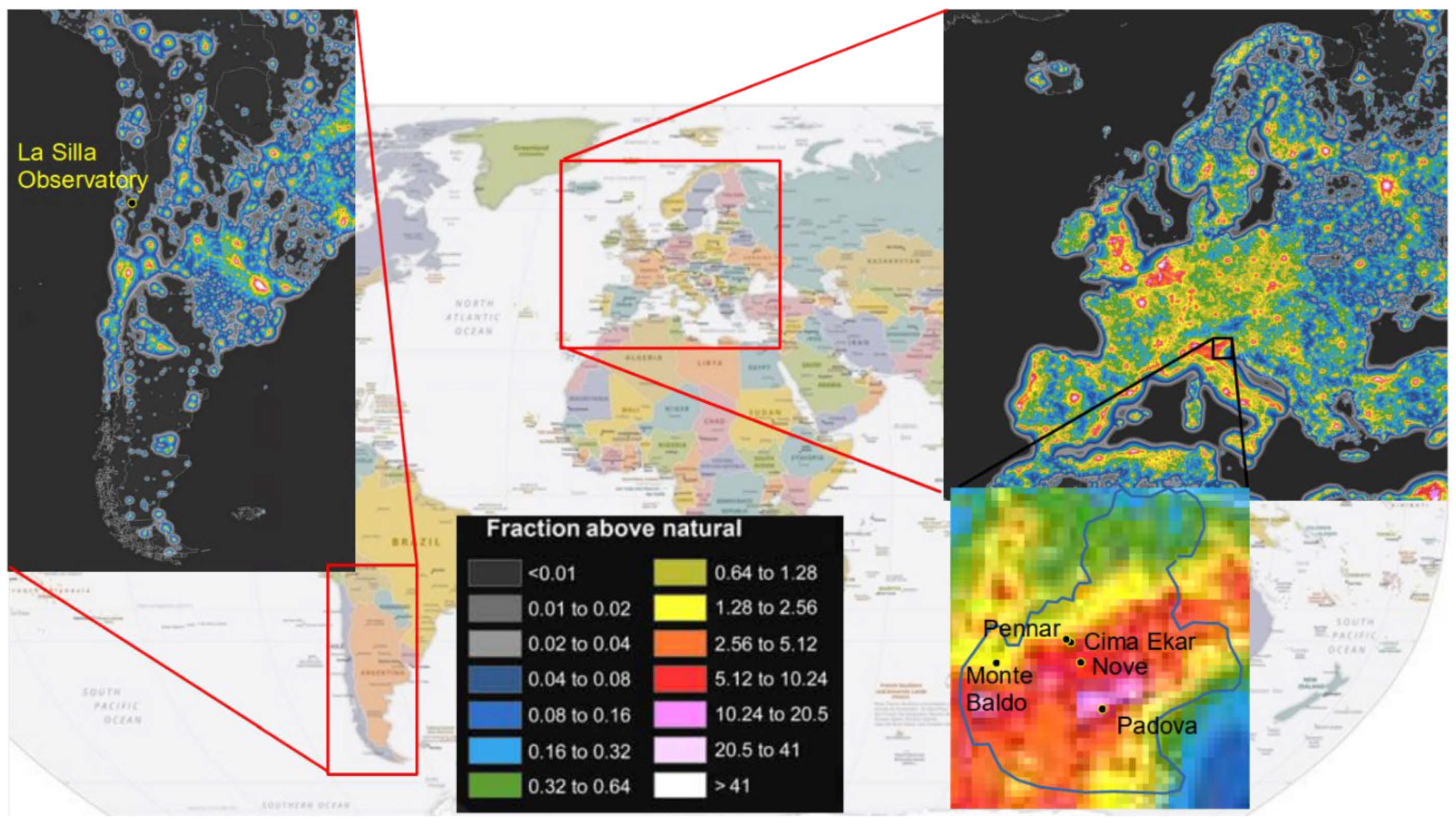
2.1. The Analysed Data

Here the data recorded by stations at sites either close to or within the Po Valley (Italy) are mainly considered. This last is the most industrialized Italian region, extending about 58,000 square kilometres and with about 20 million people. As a consequence, it is the most lit and polluted area in Italy. The long-term trend of the SQM measurements is considered very significant to track this important polluted area. The sites are placed at different altitudes from plain at few meters over the average sea level to the mountains up to several thousands of meters. At the opposite, an SQM placed in a very clean site is also analysed. It is placed at La Silla Observatory in Chile. The place is a mountain saddle at the outskirts of the Chilean Atacama Desert, one of the driest and most remote areas of the world.

Table 1. List of the considered sites and their altitude.

Site	Altitude (m)
Padova (Italia)	12
Nove (Italia)	84
Pennar (Italia)	1050
Ekar (Italia)	1366
Monte Baldo (Italia)	2218
La Silla (Chile)	2400

specifies the altitude of each considered site, while Figure 1 shows the location of the stations. The very different measuring conditions are apparent from the maps of the ratio of the artificial sky brightness over that of the natural sky obtained from [47,48]. Apart from different air pollution and light conditions, these sites have quite different atmospheric conditions, too. The data measured by the SQMs of the Veneto network are recorded every 5 min, while at La Silla the sampling period is equal to 3 min. Recording every 5 min does not assure one measurement is always acquired when the Sun places at an altitude between −7° and −6°, the sampling at 3 min rate allows every day has at least one sample at sunset and at dawn. All the SQMs present narrow field of view and a Full Width Half Maximum (HWHM) equal to 20°.

Usually, data provided by SQMs are acquired in magnitudes m, in particular m_SQM, where the subscript SQM means the measured radiance is obtained weighting the electromagnetic radiation with the spectral responsivity of that kind of instruments. Magnitudes are logarithmic with respect to the sky radiance M over the reference radiance M_ref of the manufacturer laboratory. The equation connecting those quantities is the following

$$m=-2.5lo{g}_{10}\left(\frac{M}{M_{ref}}\right).$$

(1)

Apart from a brief consideration in the Discussion section, the SQM data analysed in this work are always considered in the magnitude logarithmic scale.

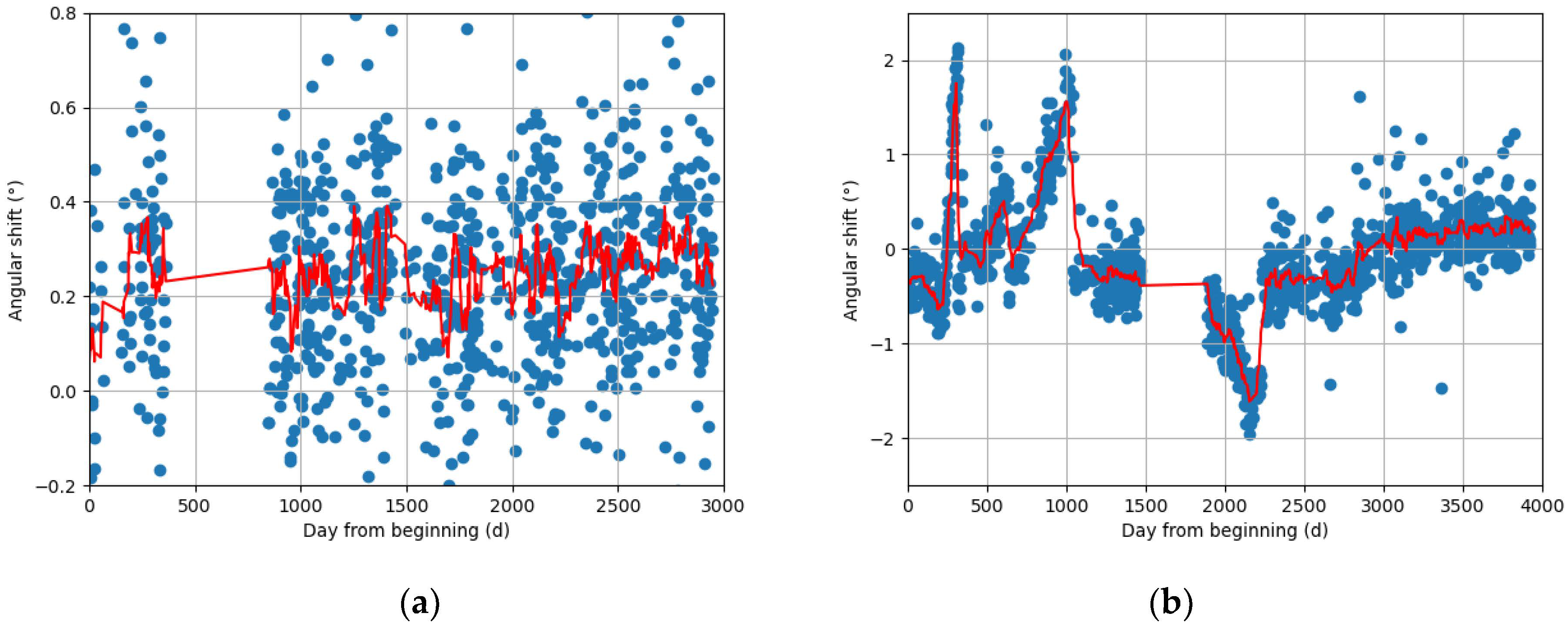
2.2. The Model of Twilight at Sunset and Dawn

We consider a multiplicative model to describe the measurement process; according to the model, the output of the SQM can be expressed as follows

$$B\left(t\right)=m\left(t\right)r\left(t\right)b\left(t\right)+\epsilon \left(t\right)$$

(2)

where

• b(t) is the brightness of the sky in defined (reference) meteorological conditions and reference status of the instrument, for example the status after a calibration or at the beginning of a time series;
• m(t) describes the effect of atmospheric conditions different from reference ones, for the latter m = 1;
• r(t) describes the effect of instrument status different from reference one, for the latter r = 1.

In the considered model, the additive term $\epsilon \left(t\right)$ is a random noise component with zero mean, when the instrument offset is considered compensated.

When the sky brightness is analysed at sunset and at dawn, the quantity b depends on time because the Sun places at different angular positions over the horizon $\alpha \left(t\right)$ (solar altitude) along its setting and rising, therefore $b\left(t\right)=b\left(\alpha \left(t\right)\right)$. When measuring the NSB at the zenith, the angular position plays a role depending to the topology, obstacles at/near the horizon.

The factor m can show either periodical or stochastic components, as time varies; as example, meteorological conditions can seasonally and yearly repeat. Furthermore, changes in meteorological conditions can present a time trend, which can cause increasing or decreasing trend of the factor m and consequently on the instrument output.

r(t) can present trends over time, too; they represent variations on the instrument. Again, they can be random or due to seasonal variations, e.g., due to temperature variation of the instrument components and therefore of their performances. They can present time trends, a possible cause can be ageing of the instrument itself: examples are reduction of window and filter transparency, reduction of the efficiency of the photodiode used to convert the collected light to the measured current.

Even if no changes on meteorological conditions and on instrument status happen, a discrepancy can appear between real sky brightness and the apparent output of the instrument. A possible cause could be an error on the clock of the system acquiring SQM data and, consequently, an incorrect timing of the sequence of brightness values, including also data at dusk and dawn. The systems acquiring data from the SQMs of the Veneto network and the SQM at La Silla use different approaches, hardware and software. In some cases, the trigger for the acquisition is provided by a PC; for other cases, a Raspberry Pi starts the acquisition; further SQMs are connected to a local network and a server asks them for the data. Consequently, there is also a wide spread about the software used to obtain the reading, ranging from the one provided by the SQM manufacturer, Unihedron, passing through dedicated codes written in Aseba for systems based on Raspberry Pi, up to codes in PL/SQL, when, a server is used. Unfortunately, not all the acquiring systems were, mainly in the past, always connected to internet and, therefore, able to adjust and to compensate the drift in their clock. These variations directly affect the timing of SQM data.

When the brightness of the sky at sunset and dawn is used to verify the calibration of SQM, for each considered day the time instants when the Sun has an altitude within the interval [−7°, −6°] is identified according to the Sun’s equations of motion. Errors on the instrument clock cause the use of wrong values of the Sun altitude and consequently of the sky brightness, the problem will be explained in details later.

Equal or similar atmospheric conditions are supposed at sunset before and dawn after a considered night. Therefore, in first approximation, variations of the factor m are the same at sunset and dawn corresponding to the same night. Obviously, the variation of the instrument status from the reference is assumed the same during the night, the sunset before and the subsequent dawn. Ageing is supposed a process with evolution time longer than few hours.

We consider small variations of m, r and b, defined $\Delta m$, $\Delta r$ and $\Delta b$, respectively. By analysing average values, so as the effect of the component $\epsilon \left(t\right)$ is zero; their correspondent variation of the instrument output is

$$\Delta B=m·r·\Delta b+m·b·\Delta r+r·b·\Delta m.$$

(3)

Remembering m = 1 and r = 1 correspond to starting conditions, the equation becomes

$$\Delta B=\Delta b+b·\Delta r+b·\Delta m.$$

(4)

If the sky brightness does not change ($\Delta b=0$), e.g., observing the sky lit by the Sun at sunset and dawn at different days, with the Sun at the same altitude angle over the horizon, we can obtain the variation of the instrument output $\Delta B$ without the possibility to discriminate between the effects of variation of the instrument response, $\Delta r$, and those due to the changes of the atmospheric conditions, $\Delta m$. They act the same way. A variation of the instrument response, e.g., due to ageing, can be detected only by either taking into account the impact of the atmosphere (e.g., [49]) or keeping the atmospheric conditions constant, e.g., by analysing the instrument in a laboratory.

In the following analysis of the brightness of the sky lit by the Sun at sunset or dawn, the two contributions can be fused in a single term, the variation of the instrument output has now the following expression:

$$\Delta B=\Delta b+b·\Delta g$$

(5)

with $\Delta g=\Delta r+\Delta m$.

The term $\Delta b$ represents the effect of the variations of the sky brightness on the instrument output, it can be different from zero even if there are no real variations of the sky brightness. Variation on the recorded output of the instrument can be caused by an error in the evaluation of the altitude angle at sunset and dawn, this last can be due to a time shift of the instrument clock. $\Delta b$ represents also this variation compared to the real sky brightness, the mechanism is as described here below.

The time instants $t\left(\alpha \right)$ when the Sun at sunset and dawn places at altitude angles within the interval [−7°, −6°] are identified from the evaluation of the Sun’s motion equations and an exact clock. These time instants are searched for among the time values recorded in the database by identifying some samples, pairs (time of the instrument clock, measured brightness). These samples are selected supposing the time values presented by the instrument are equal to the exact time. It implies the assumption that the real values of the Sun altitude angles corresponding to the measured brightness values are assumed right. Truthfully, the instrument clock is not right and shows a time shift, generally. It causes an error in the selection of the sample corresponding to the sought altitude angle $\alpha$, and a wrong link between the altitude angle $\alpha$ and the measured brightness.

Thus, we consider the example where the instrument clock lags and the delay $\Delta T$ is a positive value. The selected brightness at the sunset corresponds to a delayed Sun position, an altitude angle more negative than the supposed $\alpha$, more below the horizon than $\alpha$.

To better clarify the problem, here below different quantities are defined referring to an exact time reference and to the instrument clock:

$t$	exact local time
$\alpha$	exact Sun altitude angle
$t\left(\alpha \right)$	$\mathrm{exact} \mathrm{time} \mathrm{corresponding} \mathrm{to} \mathrm{the} \mathrm{position} \mathrm{of} \mathrm{the} \mathrm{Sun} \mathrm{at} \mathrm{the} \mathrm{altitude} \mathrm{angle} \alpha$
$B\left(\alpha \right)$	$\mathrm{brightness} \mathrm{corresponding} \mathrm{to} \alpha$
$t^{\prime }$	time shown by the clock in the instrument
$t_c=t^{\prime }+\Delta T$	time shown by the clock in the instrument corrected for the delay
${\alpha }^{\prime }$	$\mathrm{altitude} \mathrm{angle} \mathrm{corresponding} \mathrm{to} \mathrm{the} \mathrm{instrument} \mathrm{time} t^{\prime }$
$B\left({\alpha }^{\prime }\right)$	$\mathrm{brightness} \mathrm{corresponding} \mathrm{to} \mathrm{the} \mathrm{altitude} \mathrm{angle} {\alpha }^{\prime }$

The link between the altitude angle of the Sun and time can be assumed to be linear

$$\alpha =K\left(t-t_0\right)$$

(6)

where K is the slope (depending on geographic latitude) $t_0$ is the time value at which $\alpha =0$.

At sunset $K=K_s<0$, at dawn $K=K_d>0$, we can suppose $K_s=-K_d$.

Considering a site at equator latitude and a revolution of 360° in 24 h, the constant value is

$$K=K_d=-K_s=\frac{360°}{24 \mathrm{h}}=15° {\mathrm{h}}^{-1}=\frac{360}{24·60}=0.25° {\min }^{-1}.$$

(7)

According to the model, the maximum error due to time shift is for a site at low geographic latitudes, the equator; therefore, Equation (7) considers a worst-case value for the slope. This effect is less at higher geographic latitudes and during cold seasons. A better approximation should consider the effect of seasons, but up to now, it was neglected; it will be implemented in future works.

If a time delay $\Delta T$ is present, the error on the Sun altitude angle at sunset is

$$\Delta {\alpha }_s={\alpha }_s^{\prime }-{\alpha }_s=K_s\left(t_c-t_0\right)-K_s\left(t-t_0\right)=K_s\left(t_c-t\right)=K_s\left(t^{\prime }+\Delta T-t\right).$$

(8)

A time value equal to $t=t\left({\alpha }_s\right)$ is looked for in the recorded data among the time values marked by the clock of the instrument $t^{\prime }$, that way we associate that time

$$t^{\prime }=t=t\left({\alpha }_s\right)$$

(9)

to the angle ${\alpha }_s$.

Therefore, the error on the estimated altitude angle is

$$\Delta {\alpha }_s=K_s\Delta T.$$

(10)

Considering dawn, a similar argumentation holds, but $K=K_d=-K_s$, therefore the angular error at dawn is

$$\Delta {\alpha }_d=-K_s\Delta T.$$

(11)

The time shift produces an effect of the same amplitude at sunset and dawn, but with opposite sign:

$$\Delta {\alpha }_s=-\Delta {\alpha }_d=K_s\Delta T.$$

(12)

Here it is supposed that variations on the altitude angle cause proportional variation of the sky brightness at zenith. It holds when angular variations are small, in our cases within the interval [−7°, −6°], or the wider interval [−8°, −5°] sometimes involved in the analysis of the experimental data. According to the model in [50], the trends of the sky brightness at zenith for BVR Johnson-Cousins system passbands are presented in Figure 2. The line corresponding to the linear regression of data of the B filter in the interval [−8°, −5°] is also shown. The B filter case is presented as example, furthermore, this case is considered in [46] as the data are closer to the ones collected by SQMs. The regression coefficient very close to unitary value shows the goodness of the linear approximation. The difference between model and linear regression in the interval [−8°, −5°] presents a standard deviation equal to 0.030 mag arcsec⁻², that is equal to 0.22% of the mean value of the sky brightness in the analysed interval. The maximum difference between the linear approximation and the model happens at the edges of the interval and is equal to 0.059 mag arcsec⁻², and to 0.43% of the mean brightness value.

The value of about 0.2% of the standard deviation from linearity authorise the use of the linear approximation for small variation. The absolute value of the standard error is lower than the uncertainty on brightness measured by SQM declared by the manufacturer, equal to 0.1 mag arcsec⁻². The linear approximation will be used to apply a correction to the altitude angle of the Sun in the recorded database when required. Unfortunately, the time shift of the clock of some SQM acquisition systems sometimes caused an angular deviation more than 1° (please see below Figure 5b). Consequently, the Sun altitude in the analysed data was out of the range [−7°, −6°] used to verify the SQM calibration, according to [46]. As refer to the average long trend of sky brightness, the small error in the correction of the Sun altitude value is averaged within many other samples, becoming negligible, well below the limit of detectable variation of brightness, also if it is due to instrument ageing.

According to the linear approximation, the difference of brightness values at two different angular altitudes of the Sun ${\alpha }_1$ and ${\alpha }_2$ is

$$\Delta b=b_1-b_2=b\left({\alpha }_2\right)-b\left({\alpha }_1\right)=k_b\left({\alpha }_2-{\alpha }_1\right)=k_b\Delta \alpha .$$

(13)

where $k_b<0$ is the angular coefficient of the linear approximation, see Figure 2. The negative value of the angular coefficient means: when the Sun set the brightness magnitude increases, while at dawn, when the Sun rises, the brightness magnitude decreases.

Let’s consider ${\alpha }_1$ is the altitude of the Sun corresponding to an exact time value t and ${\alpha }_2$ is the altitude corresponding to the same time value t read on the instrument clock. If the instrument clock presents a time shift $\Delta T$, according to Equation (10), at sunset the variation of brightness is

$$\Delta b_s=k_b\Delta {\alpha }_s=-k_{b}K\Delta T.$$

(14)

while, according to Equation (11), at dawn the brightness variation is

$$\Delta b_d=k_b\Delta {\alpha }_d=k_{b}K\Delta T.$$

(15)

Here, it is assumed the time shift of the instrument clock does not change during the night. Usually shift in a quartz clock like the ones used in SQMs is mainly affected by temperature variations, which has usually slow time evolution, consequently the assumption should be confirmed.

The average of the brightness variations at sunset and at dawn, due to a time shift of the instrument clock is

$$\Delta b_m=\frac{\Delta b_s+\Delta b_d}{2}=\frac{\left(-k_{b}K\Delta T\right)+\left(k_{b}K\Delta T\right)}{2}=0.$$

(16)

This result means that the average between brightness values at sunset and at dawn is not influenced by the presence of a time shift of the internal clock of the instrument.

Considering the variation of the recorded brightness

$$\Delta B=\Delta b+b·\Delta g.$$

(17)

and evaluating the average (subscript m) between the recorded values at sunset and dawn, we obtain:

$$\Delta B_m=\Delta b_m+b_m·\Delta g_m=0+b_m·\Delta g_m=B_m·\Delta g_m$$

(18)

where $B_m$ is the mean of the brightness values recorded at sunset and at dawn.

Equation (18) means: the residual variation of the average of brightness at sunset and dawn is only due to long-term variation on the atmospheric conditions, assumed equal at sunset and dawn, and to variation on the instrument response. The relative variation of the average brightness, relatively to the average recorded brightness, is equal to the sum of relative variation of atmospheric effects and relative changing in the instrumentation:

$$\Delta g_m=\Delta m_m+\Delta r_m=\frac{\Delta B_m}{B_m}.$$

(19)

Neglecting atmospheric variation, this ratio represents the relative variation of the instrument.

The semi-difference of the brightness variations at sunset and at dawn is

$$\Delta b_{diff}=\frac{\Delta b_s-\Delta b_d}{2}=\frac{\left(-k_{b}K\Delta T\right)-\left(k_{b}K\Delta T\right)}{2}=-k_{b}K\Delta T.$$

(20)

From this semi-difference, we can estimate the time shift of the instrument clock:

$$\Delta T=-\frac{\Delta b_{diff}}{k_{b}K}.$$

(21)

Similarly to the procedure adopted above, considering the variations of the recorded values of brightness and analysing the semi-difference at sunset and dawn, we obtain:

$$\Delta B_{diff}=\frac{\Delta B_t-\Delta B_d}{2}=\frac{\Delta b_s-\Delta b_d}{2}+b\frac{\Delta g_s-\Delta g_d}{2}=\frac{\Delta b_s-\Delta b_d}{2}=-k_{b}K\Delta T.$$

(22)

The result holds assuming that effects of long-term atmospheric and instrument variations, relatively to reference conditions, are the same at sunset and dawn. Under this hypothesis, they do not provide any contribution to the semi-difference. The assumption is considered a good approximation for photometric and spectrometric nights; therefore, the time shift of the clock of the system acquiring SQM data can be evaluated from brightness measurements at sunset and at dawn:

$$\Delta T=-\frac{\Delta B_{diff}}{k_{b}K}.$$

(23)

What is presented above holds for the variations of measured values of the sky brightness at sunset and dawn and the variation of the clock time shift.

It is interesting to analyse what happens when considering the difference of measured brightness values instead of variations. Variations can be obtained from measurements considering as references the values of the brightness at the first sunset and dawn of the recorded time series $B_{i,0} i=s,d$. According to this approach, the brightness variations are

$$\Delta B_i^{\prime }=B_i-B_{i,0}i=s,d.$$

(24)

usually

$$B_{s,0}\ne B_{d,0}.$$

(25)

and both are different from $B_0$, the real brightness at sunset and dawn, at the same altitude angle of the Sun over the horizon. The difference between the initial values is not zero, owing to the presence of an initial shift of the instrument clock relatively to the absolute local time. The brightness variation from the real brightness at sunset and dawn, is

$$\begin{gathered} \Delta B_i=B_i-B_0=\left(B_i-B_{i,0}\right)+\left(B_{i,0}-B_0\right)=\left(B_0+\Delta b_i+B_0·\Delta g\right)-B_0= \\ \Delta b_i+B_0·\Delta gi=s,d. \end{gathered}$$

(26)

The semi-difference of the variations obtained from recorded brightness at sunset and dawn is

$$\Delta B_{diff}=\frac{\Delta B_s-\Delta B_d}{2}=\frac{\left(B_s-B_0\right)-\left(B_d-B_0\right)}{2}=\frac{B_s-B_d}{2}.$$

(27)

Equation (27) shows the semi-difference can be obtained directly from the measured brightness values. Therefore, the time shift of the internal clock can be obtained from the recorded brightness:

$$\Delta T=-\frac{\Delta B_{diff}}{k_{b}K}=-\frac{B_s-B_d}{2k_{b}K}.$$

(28)

Equation (28) allows evaluating the time shift from the first beginning of the recording.

Based on Equations (10) and (11) we can evaluate the angular shifts on the Sun altitude at sunset and dawn due to the time shift of the instrument clock:

$$\Delta {\alpha }_s=-K\frac{B_s-B_d}{2k_{b}K}=-\frac{B_s-B_d}{2k_b}. \mathrm{for} \mathrm{sunset} (\Delta {\alpha }_s>0 \mathrm{if} \Delta T>0, \frac{B_s-B_d}{2}>0)$$

(29)

and

$$\Delta {\alpha }_d=K\frac{B_s-B_d}{2k_{b}K}=-\frac{B_s-B_d}{2k_b}=-\Delta {\alpha }_t \mathrm{for} \mathrm{dawn} (\Delta {\alpha }_d<0 \mathrm{if} \Delta T>0)$$

(30)

These values can be used to correct the estimate of the altitude of the Sun associated with the selected sample according the following equations.

At sunset the error is $\Delta {\alpha }_s={\alpha }_s^{\prime }-{\alpha }_s$ therefore the corrected value is

$${\alpha }_s={\alpha }_s^{\prime }-\Delta {\alpha }_s$$

(31)

where ${\alpha }_s$ is the right angle corresponding to the measured brightness and ${\alpha }_s^{\prime }$ is the value estimated based on the time of the instrument.

At dawn the corrected value of the Sun altitude is

$${\alpha }_d={\alpha }_d^{\prime }-\left(-\Delta {\alpha }_s\right)={\alpha }_d^{\prime }+\Delta {\alpha }_s$$

(32)

where ${\alpha }_d$ is the altitude corresponding to the measured brightness and ${\alpha }_d^{\prime }$ is the value based on the instrument time.

2.3. Approaches to the Data Analysis

Two possible approaches can be considered to evaluate the trend of the drift in brightness measurements.

The first uses Equations (18) and (19) by evaluating the daily mean of brightness at sunset and dawn. The time trend of the mean brightness is considered and the regression of the data using a straight line is evaluated. This simpler model corresponds to an exponential decay of the performance of the instrument. The line slope is the ageing ratio of the instrument, if no significant variations happen in the atmospheric conditions. There is no need of comparing the measured brightness values with a model of the brightness of the sky when the Sun is below the horizon. The variation relative to the initial value of the slow trend of the measured brightness is directly linked to the instrument ageing. If no instrument ageing happens, no mean variation should be detected; apart from that due to the atmospheric variation. The only fast variability on the data shall be due to the sampling in the recording: the brightness is detected randomly relatively to the altitude angle at which the Sun stays, within the interval between −7° and −6°. The probability density of the selected angular values is uniform within this interval, if no shift appears in the instrument clock. The average action of the linear regression model allows to consider the mean trend and to dampen the variability due to the sampling and different atmospheric conditions.

The second way analyses the time change in the relationship between the altitude of the Sun below the horizon and the measured sky brightness at zenith. In the presence of ageing of the instrument, if its responsivity reduces, lower brightness values correspond to the same altitude of the Sun as time passes. Owing to the random atmospheric conditions happening when sampling the data, different measured brightness values correspond to a specific altitude value: an averaging action has to be applied to track the instrument ageing. Furthermore, the angular value of the Sun altitude corresponding to the samples presents a significant variability, it is within the interval from −7° and −6°, we don’t have always only one specific value. Examples of the recorded data corresponding to all sunsets and all dawns at Pennar are presented in Figure 3a,b, respectively. The red lines in Figure 3 show the trends for all recorded data at sunset and dawn.

We decide to group the data in subsets collecting pairs corresponding to the same year and to find the relationship between the altitude angle and measured brightness, looking for the linear regression of those data. This action averages over different atmospheric conditions and over different values of the Sun’s altitude. Considering the annual subsets, situations similar to the one presented in Figure 3 can be obtained for each year. Without any other superposed phenomena, the linear trend of the brightness versus the Sun’s altitude should show a constant angular coefficient, regardless of the instrument status and ageing. The variation of the vertical position of any point in the regression line describes the instrument ageing: reduction in the instrument responsivity corresponds to higher values of the logarithmic scale of brightness. Both the angular coefficient and the line intercept present uncertainties, they in turn define the uncertainty of the vertical coordinate of any point along the regression line. In Figure 3, the blue curves account for the uncertainty of the vertical position of each point along the regression line. The point with the minimum vertical uncertainty is the one at the average altitude angle of the analysed data set, which is always close to −6.5°. To compare the situation related to each year, the same value for the Sun’s altitude has to be considered, the average altitude angle of the whole dataset was selected for each site.

Data corresponding to sunsets and dawns of the same year were collected together, as they correspond to the same phenomenon. Difference in the atmospheric conditions causes a variability in the sky brightness, like it happens for separate data at sunset and dawn.

For example, the case of the SQM at Pennar is presented in Figure 4. Only the regression lines of the annual data are shown, highlighting the related year. The average Sun altitude angle of all data analysed for the Pennar site is about −6.51°. The dots at this angle correspond to the annual average brightness at the average considered altitude angle. All lines have quite the same slope as expected, within the interval from −1.36 mag_SQM arcsec⁻² year⁻¹ to −1.15 mag_SQM arcsec⁻² year⁻¹ and an average value of about −1.24 mag_SQM arcsec⁻² year⁻¹. The value −1.29 mag arcsec⁻² year⁻¹ of the slope of the regression line of Figure 2 is within this range, confirming the fitness of the model presented in [50] to the analysed data. The brightness values corresponding to each year were used to evaluate the trend of the instrument, it is presented in the section related to results.

Gathering data at sunset and at dawn for the annual analysis can be done directly if there is not a shift of the instrument clock relatively to the absolute local time. In this case, the recorded altitude deduced from the instrument time correspond to the real Sun’s altitude. Otherwise, recorded angular values have to be corrected by using an estimate of the time shift.

The angular error caused by the time shift may be constant or time variable. It can be obtained from the difference of the sky brightness according to Equations (27) and (28). Two examples are presented in Figure 5, they correspond to the SQMs at Pennar and Ekar observatories. The dots show the angular error evaluated for each recorded pair sunset-dawn, a great variability is apparent, it is certainly due to different atmospheric conditions. The red curve presents the average behaviour, performing an average mean over 15 days. For the Pennar site the angular shift is quite constant; on the contrary, the high instability of the clock of the SQM at Ekar caused several significant variations of the angular error which reaches the value of about ±2°.

After correcting the Sun altitude value by the angular shift, the brightness of the sky at zenith versus the Sun altitude is presented in Figure 6 for the two sites, as examples. For the Pennar site, the shift essentially moves stiffly right the block of the data corresponding to sunset and to the left that one related to dawn. The regression lines for sunset and dawn data highlight the good alignment, which is apparent also by observing the data distribution, directly. The regression lines have quite the same slope and intercept, the differences are within their respective uncertainties. A small spread of the altitude range happens, it is about twice the average angular error of 0.25°. A different situation appears for the Ekar SQM which presents strong variations in its internal clock. The spread of the recoded data brings to an angular range wide about 4°; within that interval the linear approximation of the relationship between sky brightness at zenith and Sun’s altitude becomes weaker, even if the error is still well below the measurement uncertainty declared by the manufacturer, as stated above. In this case, data corresponding to sunset are on average moved towards less negative value, on the contrary for data corresponding to dawn. According to the model described in [50] the relationship between sky brightness and altitude angle presents a smaller slope for more negative angles and an increasing slope for angle with less negative values. Those two facts cause the blue regression line corresponding to sunset data shows a slope higher than the red line related to dawn data, as it appears in Figure 6b. This difference in slope affect the minimum of the estimate of the annual trend of the instrument response as it is evaluated considering an elevation angle close to −6.5°, where the regression lines are very close to each other.

The evaluation of the mean value and of difference of the sky brightness at sunset and at dawn is possible only if a day presents data for both moments. There are days without that pair, they show recording only for sunset or for dawn; data of those days can be used approaching the problem of the drift in brightness measurements only by using the second method above described. Furthermore, correspondent Sun altitude values should be corrected for the error due to the time shift by using interpolated values.

Otherwise, an alternative to quantify slow variations in the instrument clock can be based on the analysis of sets of data corresponding to sunset and dawn recorded in the same time interval, i.e., the same year. A constant time shift along the considered time interval causes a stiff relative movement of the data corresponding to sunset and dawn along the axes of the altitude angle, as presented in Figure 6a. The regression lines of the two sets can be evaluated separately, then the correction to be applied to the estimated Sun altitude can be evaluated by imposing the alignment and superposition of the regression lines of sunset data and dawn data. This approach is always possible, even if it allows evaluating an average correction. Furthermore, when days present recording both at sunset and at dawn, this method can be used to verify the effectiveness of the correction of the time shift already applied.

3. Results

Here in the following from Figure 7, Figure 8, Figure 9, Figure 10, Figure 11 and Figure 12, the trend of the average the sky brightness at zenith at sunset and dawn is presented in panels (a) and the annual average sky brightness in panels (b) when the Sun altitude is at the average Sun altitude angle of all data analysed for each specific site, always around −6.5°.

The presentation of the results moves from the plain sites towards the mountain sites in Italy by increasing the altitude. The last result refers to the data from La Silla.

In the section (a) of each figure, the circles represent the values of the sky brightness at zenith averaged between sunset and dawn. That mean value is independent of the clock error, but can be obtained only if both data at sunset and dawn are available for the same night. To highlight the trend of the average sky brightness, the moving average of the daily values is presented by the yellow curve; for the presented figures the average is made over the samples of 4 months. Aside, the green curves account for one standard deviation of the moving mean. The moving average emphasises the slow variations probably happening in the atmospheric conditions and helps to notice the slow fluctuations also on the daily data represented by dots. They can be observed for the recordings at Padova, Ekar and La Silla. At the other sites they cannot be always seen clearly owing to a less regular availability of data and to long time with no reliable samples. Data for some days are missing, it happens for those night recordings without data both at sunset and at dawn, too. The slow variations have approximately a period of a year with superposed asynchronous components. The annual fluctuations are particularly apparent in Figure 12 for the data from La Silla. The atmospheric conditions of that wildest site are less affected by anthropic actions, consequently seasonal variations are more visible. The day by day fast fluctuations on the sky brightness superposed to the seasonal variations are attributable to daily changing in the sky conditions, but mainly to the random sampling of the data when the Sun altitude is within the angular interval between −7° and −6°.

Superposed to the daily data and the moving mean is the regression line of the daily average sky brightness. The red line in the section (a) is the linear least squares interpolation of the daily data; it is the simplest approximation of the average long-term trend of the sky brightness at twilight. The blue curves close to the regression red line account for one standard uncertainty in the determination of the line parameters slope and intercept. For each site, the values of the slope in the equation of the lines interpolating the daily data and the yearly average data are presented in

Table 2. Values of the working time and of the slope of the equation of the line interpolating the daily data for each considered site; slope column (a) consider daily data, while column (b) considers yearly average data.

Site	Working Time (y)	Slope (a) (magSQM arcsec−2 year−1)	Slope (b) (magSQM arcsec−2 year−1)
Padova (Italia)	5	0.053 ± 0.006	0.054 ± 0.013
Nove (Italia)	5	0.068 ± 0.014	0.060 ± 0.032
Pennar (Italia)	8	0.086 ± 0.006	0.088 ± 0.011
Ekar (Italia)	10	0.053 ± 0.004	0.051 ± 0.014
Monte Baldo (Italia)	7	0.086 ± 0.022	0.121 ± 0.021
La Silla (Chile)	4	0.029 ± 0.005	0.017 ± 0.013

with their uncertainty (one standard deviation).

The problem caused by the fact that only some nights can be associated to data both at sunset and dawn is apparent for the site of Monte Baldo. In Figure 11a the first recording year has only one night associated to both sunset and dawn measurement. It also prevents to evaluate the dispersion of the mean. A similar situation happens for the Nove site, the first moving average acts on twilight measurements of only 3 nights. Consequently, the dispersion on the moving average is large. The issue can be overcome by evaluating the long-term trend of the sky brightness by applying the second method above presented. The results are shown in section (b) of the Figure 6, Figure 7, Figure 8, Figure 9, Figure 10 and Figure 11. For most sites five or few more years are available, while for Pennar and Ekar 7 and 9 years are available, respectively. Each year is associated to the average sky brightness at zenith and its uncertainty, both of them are represented in the plots by dots and bars. The red line in each plot is the linear fitting accounting for the yearly average value and its uncertainty, while the blue curves account for the uncertainty on the parameters describing the regression line. As for the section (a), also here the values of the slope (m) of the interpolating lines are presented. For each site, the slope values obtained following both methods are very close and significantly equivalent when their uncertainty is considered. The largest differences are obtained for Monte Baldo and La Silla. In the first case it is apparent a lack of data at the beginning of the recording in the daily analysis, many nights are not associated to both sunset and dawn brightness values. For La Silla, the atmospheric variations cause brightness variations which are large when related to the long-term trend change, it heavily affects the results based on the average annual value; the fact is highlighted by the high value of the slope uncertainty. Furthermore, seasonal fluctuations are not really regular, consequently they are not completely compensated by an annual average action and their effects are still present in the data used to evaluate the long-term trend.

4. Discussion

Figure 6, Figure 7, Figure 8, Figure 9, Figure 10 and Figure 11 show the trends of the sky brightness in the considered sites in terms of magnitude, therefore expressed in a logarithmic scale. They present an average increase in magnitude, which corresponds to a decrease in brightness in the linear scale. Coming back to the desire of evaluating the possible ageing of the instrument, Equation (19) can be used; it is worth rewriting it in the logarithmic scale:

$$m_{SQM}=-2.5lo{g}_{10}\left(\frac{B_m+\Delta B_m}{B_{ref}}\right),$$

(33)

$$\Delta m_{SQM}=-2.5lo{g}_{10}\left(\frac{B_m+\Delta B_m}{B_{ref}}\right)-\left[-2.5lo{g}_{10}\left(\frac{B_m}{B_{ref}}\right)\right],$$

(34)

$$\Delta m_{SQM}=-2.5lo{g}_{10}\left(1+\frac{\Delta B_m}{B_m}\right)=-2.5lo{g}_{10}\left(1+\Delta g_m\right).$$

(35)

If a small variation of the parameter $\Delta g_m$ happens, the related variation in the SQM magnitude is proportional to changes in the instrument or atmospheric conditions according to the following equation:

$$\Delta m_{SQM}=-\frac{2.5}{ln10}\ln \left(1+\Delta g_m\right)\approx -\frac{2.5}{ln10}\Delta g_m$$

(36)

Subtracting from the results presented in Figure 6, Figure 7, Figure 8, Figure 9, Figure 10 and Figure 11 the sky brightness at the beginning of the recording highlights the effect of the term $\Delta g$. This contribution presents an approximately linear increase over time, in the logarithmic scale of magnitudes, the values of the increasing rate are the slopes presented in Table 2 for the considered SQM stations.

It is worth remembering that $\Delta g$ accounts for variation of the instrument response $\Delta r$ and the effects due to the variations in the atmospheric conditions $\Delta m$. At that stage, the obtained results do not allow splitting the two contributions. With the aim of knowing how ALAN affects the sky brightness as compared to a starting situation, dividing the contributions is not here significant, the evaluated results can be used to correct measured brightness at night, obtaining a better evaluation of the state of the sky, of the impact of ALAN on it and of the efficacy of actions aimed at reducing light pollution. If it is required to quantify the effects of long-term cloud and aerosol changes on NSB, further studies are needed in addition to the one presented. They should involve directly the instrument and/or the air quality.

Analysing in particular the results of the Italian sites, the increasing rate of $\Delta g$ is in the range between 50 and 90 mmag_SQM arcsec⁻² year⁻¹. Aiming at understanding the importance of these values, it may be clearer to work with a linear scale, rather than a logarithmic one. Figure 13a,b present the relative variation of the evolution of the sky brightness, $\Delta g$, for the case of the SQM at Ekar. Figure 13a shows the variation of the sky brightness at twilight due to the instrument ageing and to the changing in the atmospheric conditions in logarithmic scale; here $\Delta g$ is obtained from the moving average of the daily data, from the regression of the daily values, from the average annual values and from the regression of the average annual values. In linear scale of Figure 13b the monthly average values of the sky brightness at twilight are presented to make the image clearer, with them the moving average of the daily values and the trend corresponding to the regression over daily values are also shown. Here, the sky brightness is normalised by its value at the beginning of the recording. The linear trend in Figure 13a becomes an exponential trend in the linear scale of Figure 13b. The time constant of the exponential decay, corresponding to a slope of 53 mmag_SQM arcsec⁻² year⁻¹, is equal to about 20 years. It means, as it appears at the end of the recording of Figure 13b, the SQM output is reduced by a factor 63% after 10 working years.

Owing to the high value of the decay of the SQM output, a correction of the measured brightness is considered a need. Without any correction, false inference could be obtained from the long-term trend of sky brightness at zenith.

To correct the values of the sky brightness at night at zenith expressed in mag_SQM arcsec⁻², the variation obtained from the measurement at sunset and dawn shall be subtracted, while operating in a linear scale the sky brightness shall be divided by $\Delta g$.

For any site, a correction term shall be defined, as it is determined by the specific ageing of the instrument and by the local variation of the atmospheric conditions.

Depending on the available data, the correction can be obtained following the different ways here presented. If a regular flux of daily data is available, the correction term can be directly derived by a moving average of daily values at twilight. Changing the time duration of the window used for the average action the correction can account for faster or slower atmospheric variations. In the examples presented in this work, the width of the window is long 4 months, allowing to consider seasonal variations; they can be clearly seen in Figure 12a. Too short window used in the moving average do not provide enough smoothing action on the random variation on the daily data, in particular on fluctuation due to the casual sampling of the sky brightness values when the Sun altitude is within the interval between −7° and −6°, the effect of which have to be reduced to the minimum.

If less regular daily data are available, averaging over a year can allow accounting for slow atmospheric variations loosing seasonal changes and accounting for the instrument ageing, which seems to have a slow trend according to the analysed data.

Fitting either daily or monthly or annual data by a regression line makes a heavier average action, it is performed over all the recording interval, therefore both seasonal and annual atmospheric variations are not described in the fitting. The trend obtained from the regression fitting accounts for very slow variations, among which there are those associated to possible ageing of the instrument.

However, as it appears in Figure 6, Figure 7, Figure 8, Figure 9, Figure 10 and Figure 11 and clearer in Figure 12, in the analysis of the long-term trend the different approaches in evaluating the tendency and the correction term bring to similar results, all they are useful to correct a measurement error and to reach a better understanding of the effect of ALAN on NSB.

Commenting Figure 13 shows the importance of the correction, it can be further highlighted by analysing the trend of the values of the night sky brightness directly.

For example, Figure 14 presents by the blue symbols and lines the monthly modal values of the night sky brightness measured at Ekar and their moving average with a 4 months wide window. Here, the mode is evaluated as the average value of the NSB measurements, the peak of which is within the full width at half-maximum interval of the clear nights’ peak [18]. It is apparent the raw data would exhibit a trend towards darker sky, the regression line presented with its one standard deviation uncertainty band has a slope of 30 mmag_SQM arcsec⁻² year⁻¹.

That trend can be compared with the estimated drift associated to the variation of the installed luminous flux used for outdoor public lighting; this last is expected to have an increase of about 10% in the years from 2014 to 2021 in Veneto, as it presented in [51]. In logarithmic scale it would correspond to a variation of about −15 mmag_SQM arcsec⁻² year⁻¹, or 1.4% per year in linear scale, if the fraction of upward luminous flux does not vary and by neglecting the dimming of outdoor lighting. The expected trend is represented by the grey dashed line of Figure 14. The reduction of the measured sky brightness seems to be in opposition with this expected increase on the luminous flux.

The values of the measured brightness were corrected by the term obtained from the moving average of the daily data at twilight, which are shown in Figure 13. Those adjusted values are presented in Figure 14 by the magenta symbols and average line; furthermore, the red regression line shows the average tendency. The correction term changes the drift in the opposite direction, i.e., towards a more light polluted sky. The slope in the equation of the fitting line changes from positive to the negative value of −21 mmag_SQM arcsec⁻² year⁻¹. In linear scale it corresponds to an increase of about 2% per year, which is in the same direction of the expected increment of the installed luminous flux, even bigger; it may be due to variation in private outdoor lighting.

The trend of $\Delta g$ has a significant exponential component very similar to typical ageing trend of material properties, in our case they could be the transmittance of instrument windows and filters, something was analysed in [51], and the efficiency of the photodiode conversion. Up to now it is not clear what could be the decay phenomenon, it may be connected to solar exposition, in particular UV and radiation at short wavelengths. In particular, possible causes of the performances decay could be the irradiance on the instruments during daytime. This hypothesis has to be verified. Furthermore, at La Silla there could be a double value of the irradiance exposition owing to higher altitude of that site than on the Italian ones and cleaner atmosphere, on the contrary the presented results show the lower increasing rate of measured sky brightness at sunset and dawn.

A detailed analysis of the SQMs in laboratory conditions should be required to assess their ageing, but to grant the continuity of the measurements it was chosen not to remove any SQM from the Veneto network and performing their maintenance or substituting an instrument only when it is strictly required. Within that management strategy, it is considered interesting to develop a portable system able to perform simple tests also on site. Clearly, they will be less accurate, on the other side they could be done regularly following the time evolution of the instruments and detecting its ageing. In this way, it is also possible to better identify the contribution of atmospheric variations in the brightness measurements of the night sky.

5. Conclusions

The use of Sunlight at twilight as calibrator is particularly interesting when the measurements are collected both at sunset and at dawn. The average of the two measures recorded at the turn of the same night allows to compensate possible time drift in the internal clock of the instruments. Considering only one of the two acquisitions may cause misleading results caused by uncertainties of the time provided by the instrument.

The work shows the mean of the measured sunset and dawn sky brightness is independent of the clock shift, consequently it can be directly used to verify the long-term stability of the instrument. The difference of the measured sky brightness values at sunset and down is also useful, it is proportional to the shift of the internal clock of the instrument. It can be used to correct the estimated Sun altitude used in the calibration method, in case, for the specific night.

Two ways to analyse the long-term stability of the instrument are proposed: the first considers the day by day behaviour of the twilight measurements, the second analyses the data collected each year. As stated above, the day by day study allows the assessment of the instrument with high temporal resolution. Otherwise, analysing the samples of each year together averages seasonal changing in the atmosphere, but already allows compensating the average clock shift.

The analysis of the trend of the measurements at twilight cannot separate the effect of instrument ageing from the influences of atmospheric changes. However, the slow found movement is very similar to ageing behaviour of material properties, consequently it could be associated mainly to the instrument ageing.

From the analysis of SQM measurements at twilight, trends in the decay of the performances of the instruments clearly appear. The same measures also show that variations of the atmospheric conditions play a different role in air polluted and unpolluted sky. The importance of air components on SQM measures is not studied in this work, even if it is also considered interesting for the calibration issue and is foreseen in future works.

The variation, in particular the supposed decay, of the instrument performance detected by the twilight calibration method ranges between about 30 to less than 90 mmag_SQM arcsec⁻² year⁻¹. In linear scale, it corresponds to a reduction at 50% of the signal after about 8 years, in the worst case. Therefore, it is considered of such a magnitude that applying a correction term to measurements obtained from SQM constantly exposed to elements, Sun irradiance and bad weather, is required if we wish to track the sky brightness for long time. Without the correction, SQMs can no longer be used to track the effect of actions on artificial outdoor lighting systems for time longer than a few years.

Applying the twilight method requires acquiring SQM measurements not only during the night, but also at sunset and dawn across the considered night. Wishing to switch off SQMs during daytime, the instruments shall be turned on at least at sunset and kept on until the first light of the new day.

Different sites were analysed in the present work, in particular located in the most industrialised area in Italy and close to the remote Chilean Atacama Desert. The related results show different behaviours, suggesting varied influence of the air and atmospheric conditions. Future works will address that issue. Furthermore, the authors suggest the presented procedure is applied to other SQMs in different sites and atmospheric conditions to assess their effect on the instrument calibration and correction of measured night sky brightness.

References

1. Tsao, J.Y.; Waide, P. The world’s appetite for light: Empirical data and trends spanning three centuries and six continents. Leukos 2010, 6, 259–281. [Google Scholar] [CrossRef] [Green Version]
2. Jägerbrand, A.K. New Framework of Sustainable Indicators for Outdoor LED (Light Emitting Diodes) Lighting and SSL (Solid State Lighting). Sustainability 2015, 7, 1028–1063. [Google Scholar] [CrossRef] [Green Version]
3. Steinbach, R.; Perkins, C.; Tompson, L.; Johnson, S.; Armstrong, B.; Green, J.; Grundy, C.; Wilkinson, P.; Edwards, P. The effect of reduced street lighting on road casualties and crime in England and Wales: Controlled interrupted time series analysis. J. Epidemiol. Community Health 2015, 69, 1118–1124. [Google Scholar] [CrossRef] [PubMed]
4. Pust, P.; Schmidt, P.J.; Schnick, W. A revolution in lighting. Nat. Mater. 2015, 14, 454–458. [Google Scholar] [CrossRef] [PubMed]
5. Gaston, K.J.; Bennie, J.; Davies, T.W.; Hopkins, J. The ecological impacts of nighttime light pollution: A mechanistic appraisal. Biol. Rev. 2013, 88, 912–927. [Google Scholar] [CrossRef]
6. Gaston, K.J.; Visser, M.E.; Hölker, F. The biological impacts of artificial light at night: The research challenge. Philos. Trans. R. Soc. B Biol. Sci. 2015, 370, 20140133. [Google Scholar] [CrossRef] [Green Version]
7. Bennie, J.; Davies, T.W.; Cruse, D.; Gaston, K.J. Ecological effects of artificial light at night on wild plants. J. Ecol. 2016, 104, 611–620. [Google Scholar] [CrossRef] [Green Version]
8. Gaston, K.J.; Holt, L.A. Nature, extent and ecological implications of night-time light from road vehicles. J. Appl. Ecol. 2018, 55, 2296–2307. [Google Scholar] [CrossRef] [Green Version]
9. Desouhant, E.; Gomes, E.; Mondy, N.; Amat, I. Mechanistic, ecological, and evolutionary consequences of artificial light at night for insects: Review and prospective. Entomol. Exp. Et Appl. 2019, 167, 37–58. [Google Scholar] [CrossRef] [Green Version]
10. Sanders, D.; Frago, E.; Kehoe, R.; Patterson, C.; Gaston, K.J. A meta-analysis of biological impacts of artificial light at night. Nat. Ecol. Evol. 2021, 5, 74–81. [Google Scholar] [CrossRef] [PubMed]
11. American Medical Association Press Releases: AMA Adopts Guidance to Reduce Harm from High Intensity Street Lights. Available online: https://www.ama-assn.org/press-center/press-releases/ama-adopts-guidance-reduce-harm-high-intensity-street-lights (accessed on 20 August 2022).
12. Hatori, M.; Gronfier, C.; Van Gelder, R.N.; Bernstein, P.S.; Carreras, J.; Panda, S.; Marks, F.; Sliney, D.; Hunt, C.E.; Hirota, T.; et al. Global rise of potential health hazards caused by blue light-induced circadian disruption in modern aging societies. NPJ Aging Mech. Dis. 2017, 3, 9. [Google Scholar] [CrossRef] [Green Version]
13. Riegel, K.W. Light pollution: Outdoor lighting is a growing threat to astronomy. Science 1973, 179, 1285–1291. [Google Scholar] [CrossRef] [PubMed]
14. Gaston, K.J.; Davies, T.W.; Bennie, J.; Hopkins, J. Reducing the ecological consequences of night-time light pollution: Options and developments. J. Appl. Ecol. 2012, 49, 1256–1266. [Google Scholar] [CrossRef] [Green Version]
15. Aubé, M.; Roby, J. Sky brightness levels before and after the creation of the first International Dark Sky Reserve, Mont-Mégantic Observatory, Québec, Canada. J. Quant. Spectrosc. Radiat. Transf. 2014, 139, 52–63. [Google Scholar] [CrossRef]
16. Hänel, A.; Posch, T.; Ribas, S.J.; Aubé, M.; Duriscoe, D.; Jechow, A.; Kollath, Z.; Lolkema, D.E.; Moore, C.; Schmidt, N.; et al. Measuring night sky brightness: Methods and challenges. J. Quant. Spectrosc. Radiat. Transf. 2018, 205, 278–290. [Google Scholar] [CrossRef] [Green Version]
17. Bertolo, A.; Binotto, R.; Ortolani, S.; Sapienza, S. Measurements of Night Sky Brightness in the Veneto Region of Italy: Sky Quality Meter Network Results and Differential Photometry by Digital Single Lens Reflex. J. Imaging 2019, 5, 56. [Google Scholar] [CrossRef] [PubMed] [Green Version]
18. Bará, S.; Lima, R.C.; Zamorano, J. Monitoring Long-Term Trends in the Anthropogenic Night Sky Brightness. Sustainability 2019, 11, 3070. [Google Scholar] [CrossRef] [Green Version]
19. Jechow, A.; Ribas, S.J.; Domingo, R.C.; Hölker, F.; Kolláth, Z.; Kyba, C.C. Tracking the dynamics of skyglow with differential photometry using a digital camera with fisheye lens. J. Quant. Spectrosc. Radiat. Transf. 2018, 209, 212–223. [Google Scholar] [CrossRef] [Green Version]
20. Fiorentin, P.; Bertolo, A.; Cavazzani, S.; Ortolani, S. Calibration of digital compact cameras for sky quality measures. J. Quant. Spectrosc. Radiat. Transf. 2020, 255, 107235. [Google Scholar] [CrossRef]
21. Barducci, A.; Marcoionni, P.; Pippi, I.; Poggesi, M. Effects of light pollution revealed during a nocturnal aerial survey by two hyperspectral imagers. Appl. Opt. 2003, 42, 4349–4361. [Google Scholar] [CrossRef]
22. Kuechly, H.U.; Kyba, C.C.; Ruhtz, T.; Lindemann, C.; Wolter, C.; Fischer, J.; Hölker, F. Aerial survey and spatial analysis of sources of light pollution in Berlin, Germany. Remote Sens. Environ. 2012, 126, 39–50. [Google Scholar] [CrossRef]
23. Hale, J.D.; Davies, G.; Fairbrass, A.J.; Matthews, T.J.; Rogers, C.D.; Sadler, J.P. Mapping lightscapes: Spatial patterning of artificial lighting in an urban landscape. PLoS ONE 2013, 8, e61460. [Google Scholar] [CrossRef] [PubMed] [Green Version]
24. Fiorentin, P.; Bettanini, C.; Lorenzini, E.; Aboudan, A.; Colombatti, G.; Ortolani, S.; Bertolo, A. Minlu: An Instrumental Suite for Monitoring Light Pollution from Drones or Airballoons. In Proceedings of the 2018 5th IEEE International Workshop on Metrology for AeroSpace (MetroAeroSpace), Rome, Italy, 20–22 June 2018; pp. 274–278. [Google Scholar]
25. Fiorentin, P.; Bettanini, C.; Bogoni, D. Calibration of an Autonomous Instrument for Monitoring Light Pollution from Drones. Sensors 2019, 19, 5091. [Google Scholar] [CrossRef] [PubMed] [Green Version]
26. Bouroussis, C.A.; Topalis, F.V. Assessment of outdoor lighting installations and their impact on light pollution using unmanned aircraft systems-The concept of the drone-gonio-photometer. J. Quant. Spectrosc. Radiat. Transf. 2020, 253, 107155. [Google Scholar] [CrossRef]
27. Ocaña, F.; de Miguel, A.S.; Conde, A. Low Cost Multi-Purpose Balloon-Borne Platform for Wide-Field Imaging and Video Observation. In Ground-based and Airborne Telescopes VI. Proceedings of the International Society for Optics and Photonics, 2016; SPIE: Bellingham, WA, USA, 2016; p. 99061X. [Google Scholar]
28. Bettanini, C.; Fiorentin, P.; Dumitriu, A.; Accatino, F.; Cagnato, E.; Kahol, O.; Ghedin, M.; Celadin, D.; Magro, N.; Bedendo, M.; et al. Design and Test of Autonomous Scientific Payloads for Sounding Balloons. In Proceedings of the 2020 IEEE 7th International Workshop on Metrology for AeroSpace (MetroAeroSpace), Pisa, Italy, 22–24 June 2020; pp. 469–474. [Google Scholar]
29. Miller, S.D.; Straka, W., III; Mills, S.P.; Elvidge, C.D.; Lee, T.F.; Solbrig, J.; Walther, A.; Heidinger, A.K.; Weiss, S.C. Illuminating the Capabilities of the Suomi National Polar-Orbiting Partnership (NPP) Visible Infrared Imaging Radiometer Suite (VIIRS) Day/Night Band. Remote Sens. 2013, 5, 6717–6766. [Google Scholar] [CrossRef] [Green Version]
30. Kyba, C.C.M.; Garz, S.; Kuechly, H.; De Miguel, A.S.; Zamorano, J.; Fischer, J.; Hölker, F. High-Resolution Imagery of Earth at Night: New Sources, Opportunities and Challenges. Remote Sens. 2015, 7, 1–23. [Google Scholar] [CrossRef] [Green Version]
31. Estrada-García, R.; García-Gil, M.; Acosta, L.; Bará, S.; Sanchez-de-Miguel, A.; Zamorano, J. Statistical modelling and satellite monitoring of upward light from public lighting. Light. Res. Technol. 2016, 48, 810–822. [Google Scholar] [CrossRef] [Green Version]
32. Kyba, C.C.; Kuester, T.; Sánchez de Miguel, A.; Baugh, K.; Jechow, A.; Hölker, F.; Bennie, J.; Elvidge, C.D.; Gaston, K.J.; Guanter, L. Artificially lit surface of Earth at night increasing in radiance and extent. Sci. Adv. 2017, 3, e1701528. [Google Scholar] [CrossRef] [Green Version]
33. Cavazzani, S.; Ortolani, S.; Bertolo, A.; Binotto, R.; Fiorentin, P.; Carraro, G.; Zitelli, V. Satellite measurements of artificial light at night: Aerosol effects. Mon. Not. R. Astron. Soc. 2020, 499, 5075–5089. [Google Scholar] [CrossRef]
34. Cinzano, P. Night Sky Photometry with Sky Quality Meter. ISTIL Intern. Rep. 2005, 9, 1. [Google Scholar]
35. Pun, C.S.J.; So, C.W. Night-sky Brightness monitoring in Hong Kong: A city-wide light pollution assessment. Environ. Monit. Assess. 2012, 184, 2537–2557. [Google Scholar] [CrossRef]
36. Kyba, C.C.M.; Ruhtz, T.; Fischer, J.; Hölker, F. Red is the new black: How the colour of urban skyglow varies with cloud cover. Mon. Not. R. Astron. Soc. 2012, 425, 701–708. [Google Scholar] [CrossRef] [Green Version]
37. Espey, B.; McCauley, J. Initial Irish light pollution measurements and a new Sky Quality Meter-based data logger. Light. Res. Technol. 2014, 46, 67–77. [Google Scholar] [CrossRef]
38. Posch, T.; Binder, F.; Puschnig, J. Systematic measurements of the night sky brightness at 26 locations in Eastern Austria. J. Quant. Spectrosc. Radiat. Transf. 2018, 211, 144–165. [Google Scholar] [CrossRef] [Green Version]
39. Kyba, C.C.; Tong, K.P.; Bennie, J.; Birriel, I.; Birriel, J.J.; Cool, A.; Danielsen, A.; Davies, T.W.; Peter, N.; Edwards, W.; et al. Worldwide variations in artificial skyglow. Sci. Rep. 2015, 5, 8409. [Google Scholar] [CrossRef] [Green Version]
40. Zamorano, J.; Garcia, C.; Tapia, C.; Sanchez de Miguel, A.; Pascual, S.; Gallego, J. Star4all night sky brightness photometer. Int. J. Sustain. Light. 2016, 18, 49–54. [Google Scholar] [CrossRef] [Green Version]
41. Bará, S. Anthropogenic disruption of the night sky darkness in urban and rural areas. R. Soc. Open Sci. 2016, 3, 160541. [Google Scholar] [CrossRef] [Green Version]
42. Bartolomei, M.; Olivieri, L.; Bettanini, C.; Cavazzani, S.; Fiorentin, P. Verification of Angular Response of Sky Quality Meter with Quasi-Punctual Light Sources. Sensors 2021, 21, 7544. [Google Scholar] [CrossRef]
43. Cavazzani, S.; Ortolani, S.; Bertolo, A.; Binotto, R.; Fiorentin, P.; Carraro, G.; Saviane, I.; Zitelli, V. Sky Quality Meter and satellite correlation for night cloud-cover analysis at astronomical sites. Mon. Not. R. Astron. Soc. 2020, 493, 2463–2471. [Google Scholar] [CrossRef] [Green Version]
44. Robles, J.; Zamorano, J.; Pascual, S.; Sánchez de Miguel, A.; Gallego, J.; Gaston, K.J. Evolution of Brightness and Color of the Night Sky in Madrid. Remote Sens. 2021, 13, 1511. [Google Scholar] [CrossRef]
45. Schnitt, S.; Ruhtz, T.; Fischer, J.; Hölker, F.; Kyba, C.C.M. Temperature stability of the sky quality meter. Sensors 2013, 13, 12166–12174. [Google Scholar] [CrossRef] [PubMed]
46. Puschnig, J.; Näslund, M.; Schwope, A.; Wallner, S. Correcting sky-quality-meter measurements for ageing effects using twilight as calibrator. Mon. Not. R. Astron. Soc. 2021, 502, 1095–1103. [Google Scholar] [CrossRef]
47. Falchi, F.; Cinzano, P.; Duriscoe, D.; Kyba, C.C.; Elvidge, C.D.; Baugh, K.; Portnov, B.A.; Rybnikova, N.A.; Furgoni, R. The new world atlas of artificial night sky brightness. Sci. Adv. 2016, 2, e1600377. [Google Scholar] [CrossRef] [PubMed] [Green Version]
48. The World Factbook-CIA Maps. Available online: https://www.cia.gov/the-world-factbook/maps/ (accessed on 20 August 2022).
49. Puschnig, J.; Wallner, S.; Schwope, A.; Näslund, M. Long-term trends of light pollution assessed from SQM measurements and an empirical atmospheric model. Mon. Not. R. Astron. Soc. 2022, stac3003. [Google Scholar] [CrossRef]
50. Patat, F.; Ugolnikov, O.S.; Postylyakov, O.V. UBVRI twilight sky brightness at ESO-Paranal. Astron. Astrophys. 2006, 455, 385–393. [Google Scholar] [CrossRef] [Green Version]
51. Fiorentin, P.; Cavazzani, S.; Ortolani, S.; Bertolo, A.; Binotto, R. Instrument assessment and atmospheric phenomena in relation to the night sky brightness time series. Measurement 2022, 191, 110823. [Google Scholar] [CrossRef]
Figure 1. Location of the stations analysed in this work. The image is obtained processing data from [47,48].
Remotesensing 14 05787 g001
Figure 2. Trends of the sky brightness at zenith for BVR Johnson-Cousins system passbands according to the model presented in [50] and of the linear approximation of the model related to the B filter in the interval [−8°, −5°].
Remotesensing 14 05787 g002
Figure 3. Recorded data corresponding to all sunsets (a) and all dawn (b) at Pennar Observatory.
Remotesensing 14 05787 g003
Figure 4. Regression lines of data collected at sunset and dawn at Pennar grouped by years.
Remotesensing 14 05787 g004
Figure 5. Angular error at sunset caused by the time shift evaluated from the difference of the sky brightness at sunset and at dawn, (a) at Pennar and (b) at Ekar.
Remotesensing 14 05787 g005
Figure 6. Sky brightness versus Sun’s altitude corrected by the angular error caused by the time shift at Pennar (a) and at Ekar (b).
Remotesensing 14 05787 g006
Figure 7. Trends of the sky brightness at zenith at Padova: average values at sunset and dawn (a) with their moving average (yellow curve) and aside the green curves accounting for one standard deviation (a) and the annual average values (b) when the Sun altitude is around −6.5°, the red line is the linear fitting and the blue curves account for the uncertainty on the fitting parameters.
Remotesensing 14 05787 g007
Figure 8. Trends of the sky brightness at zenith at Nove: average values at sunset and dawn (a) with their moving average (yellow curve) and aside the green curves accounting for one standard deviation (a) and the annual average values (b) when the Sun altitude is around −6.5°, the red line is the linear fitting and the blue curves account for the uncertainty on the fitting parameters.
Remotesensing 14 05787 g008
Figure 9. Trends of the sky brightness at zenith at Pennar: average values at sunset and dawn (a) with their moving average (yellow curve) and aside the green curves accounting for one standard deviation (a) and the annual average values (b) when the Sun altitude is around −6.5°, the red line is the linear fitting and the blue curves account for the uncertainty on the fitting parameters.
Remotesensing 14 05787 g009
Figure 10. Trends of the sky brightness at zenith at Ekar: average values at sunset and dawn (a) with their moving average (yellow curve) and aside the green curves accounting for one standard deviation (a) and the annual average values (b) when the Sun altitude is around −6.5°, the red line is the linear fitting and the blue curves account for the uncertainty on the fitting parameters.
Remotesensing 14 05787 g010
Figure 11. Trends of the sky brightness at zenith at Monte Baldo: average values at sunset and dawn (a) with their moving average (yellow curve) and aside the green curves accounting for one standard deviation (a) and the annual average values (b) when the Sun altitude is around −6.5°, the red line is the linear fitting and the blue curves account for the uncertainty on the fitting parameters.
Remotesensing 14 05787 g011
Figure 12. Trends of the sky brightness at zenith at La Silla: average values at sunset and dawn (a) with their moving average (yellow curve) and aside the green curves accounting for one standard deviation (a) and the annual average values (b) when the Sun altitude is around −6.5°, the red line is the linear fitting and the blue curves account for the uncertainty on the fitting parameters.
Remotesensing 14 05787 g012
Figure 13. Variation of the sky brightness at Ekar site at twilight due to the instrument ageing and the changing in the atmospheric conditions, in the logarithmic scale (a) and in linear scale (b).
Remotesensing 14 05787 g013
Figure 14. Monthly modal value of night sky brightness at Ekar. In blue the measured values, their average trend and linear fitting, in magenta the corrected values and their fitting in red; m is the slope of the fitting lines in magSQM arcsec−2 year−1. In dashed grey line is the expected trend due to increase on installed outdoor luminous flux.
Remotesensing 14 05787 g014