Coral Reef Benthos Classification Using Data from a Short-Range Multispectral Sensor

Abstract

A five-band short-range multispectral sensor (MicaSense RedEdge-M) was adapted to an underwater housing and used to obtain data from coral reef benthos. Artificial illumination was required to obtain data from most of the spectral range of the sensor; the optimal distance for obtaining these data was 0.5 m, from the sensor to the bottom. Multispectral orthomosaics were developed using structure-from-motion software; these have the advantage of producing ultra-high spatial resolution (down to 0.4 × 0.4 mm/pixel) images over larger areas. Pixel-based supervised classification of a multispectral (R, G, B, RE bands) orthomosaic accurately discriminated among different benthic components; classification schemes defined 9 to 14 different benthic components such as brown algae, green algae, sponges, crustose coralline algae, and different coral species with high accuracy (up to 84% overall accuracy, and 0.83 for Kappa and Tau coefficients). The least useful band acquired by the camera for this underwater application was the near-infrared (820–860 nm) associated with its rapid absorption in the water column. Further testing is required to explore possible applications of these multispectral orthomosaics, including the assessment of the health of coral colonies, as well as the automation of their processing.

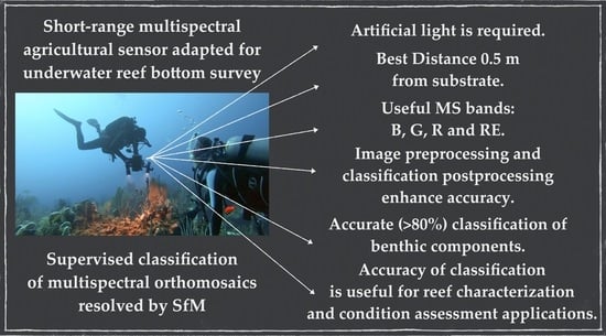
1. Introduction

Coral reef characterization, assessment, and mapping efforts rely increasingly on imagery; being digital photographs, video, or remotely sensed images. These datasets provide the means for estimating, measuring, and identifying many reef components at several scales, from species identification (cm²), percent cover of benthic components (m²), to reef habitats, geomorphology, and bathymetry (from ha to km²) [1].

The sustainable management of coral reef systems depends on scientifically validated datasets (regarding reefs’ condition, function, and structure), and specifically, on the availability of these datasets in a timely manner. On the one hand, direct observation methods such as the Atlantic and Gulf Rapid Reef Assessment protocol (AGRRA) [2], provide useful reef assessment data shortly after fieldwork, but require at least a 6-person team of highly trained observers, and assessments over large areas are time-consuming. On the other hand, imagery-based methods are quicker in the field, but imaging equipment can be cost-prohibitive, and in general, these approaches have longer data processing and product availability times. In this context, a positive trait of these imagery-based methods is that they generate permanent records that can be analyzed repeatedly and have the potential to answer future questions, different from the original question for which the imagery was collected.

In the last two decades, the implementation and advancement of the use of digital underwater photogrammetric techniques [3,4,5,6,7] coupled with the general availability of structure from motion software (SfM, i.e., Agisoft’s Metashape Pro, Pix4D), has led to strong research lines on a wide range of applications, from coral colonies characterization to applications for reef benthos assessment and ecological hypothesis testing [8,9,10,11,12,13,14,15,16], taking in-situ imagery records to a new analytic level, supported by the accurate re-creation of benthic features in ultra-high spatial resolution and combined with 3D perspectives.

A widely adopted approach for coral reef characterization is the use of multispectral imagery from satellites and airborne sensors. These tools have demonstrated their value in the past decades, in many different applications such as mapping reef habitats, bathymetry, reef structural parameters, and prediction of fish biodiversity and biomass [17,18,19,20,21,22,23,24]. They also have spawned several research topics for data correction associated with the behavior of light in the water column as surface sun-glint [25,26], light extinction in the water column [27,28,29,30,31], etc. These multispectral images are generated by passive-optical sensors which require an external energy source, and these images provide numeric data representing the intensity of different ranges of electromagnetic spectra reflected on the surface, which allows discrimination of different materials [32].

Notwithstanding the advancement in remotely sensed imagery for coral reef applications, underwater optical discrimination of materials is uncommon. This approach has two main avenues: hyperspectral analysis, defining spectral signatures, which has a long research tradition [33,34,35,36]; and multispectral analysis, which traditionally has been hindered by the availability of adequate sensors, the variability in sunlight-incidence on the bottom associated both to light extinction (solar energy absorption related to depth), and to the changes in illumination intensity due to water surface dynamics [1,37].

Nevertheless, earlier tests of methods and equipment [3,38,39,40,41,42] (among others) built a relevant knowledge base concerning the multispectral discrimination and classification of reef benthic components. These studies have motivated the goal of this study: To test the underwater use of a narrow-band multispectral sensor for reef benthos classification; with the following associated specific objectives: (a) to test the adequate operation of the sensor adapted in an underwater housing, (b) to test the need and usefulness of artificial illumination, (c) to test the appropriate image-capture distance from the bottom, (d) to test the adequacy of the underwater multispectral orthomosaics to classify benthos components, and (e) to compare the results of different supervised classification algorithms applied to the multispectral orthomosaics. The results reveal insights into the optimal approach to underwater multispectral image acquisition and facilitate accurate percent cover measurements of reef benthos components.

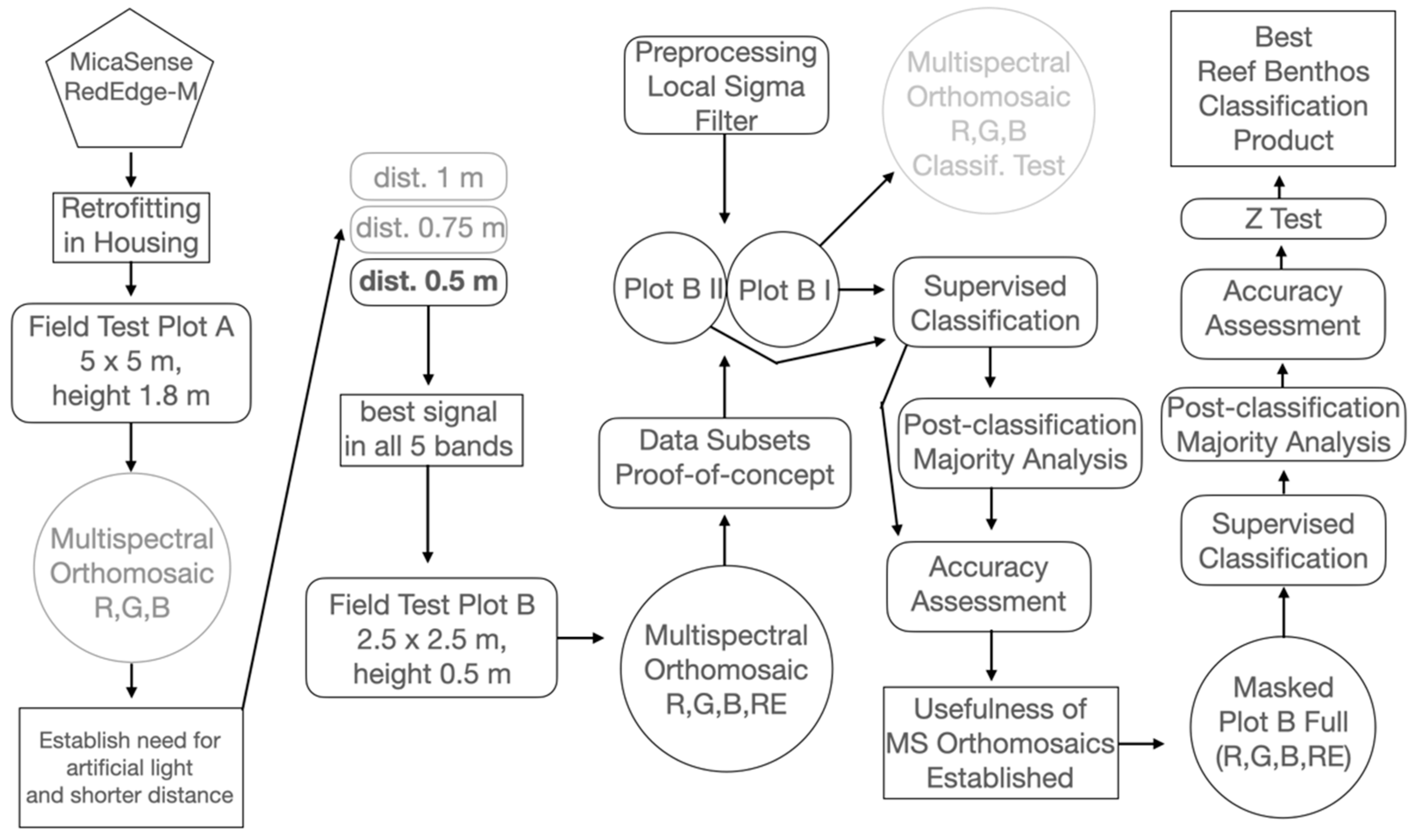
2. Materials and Methods

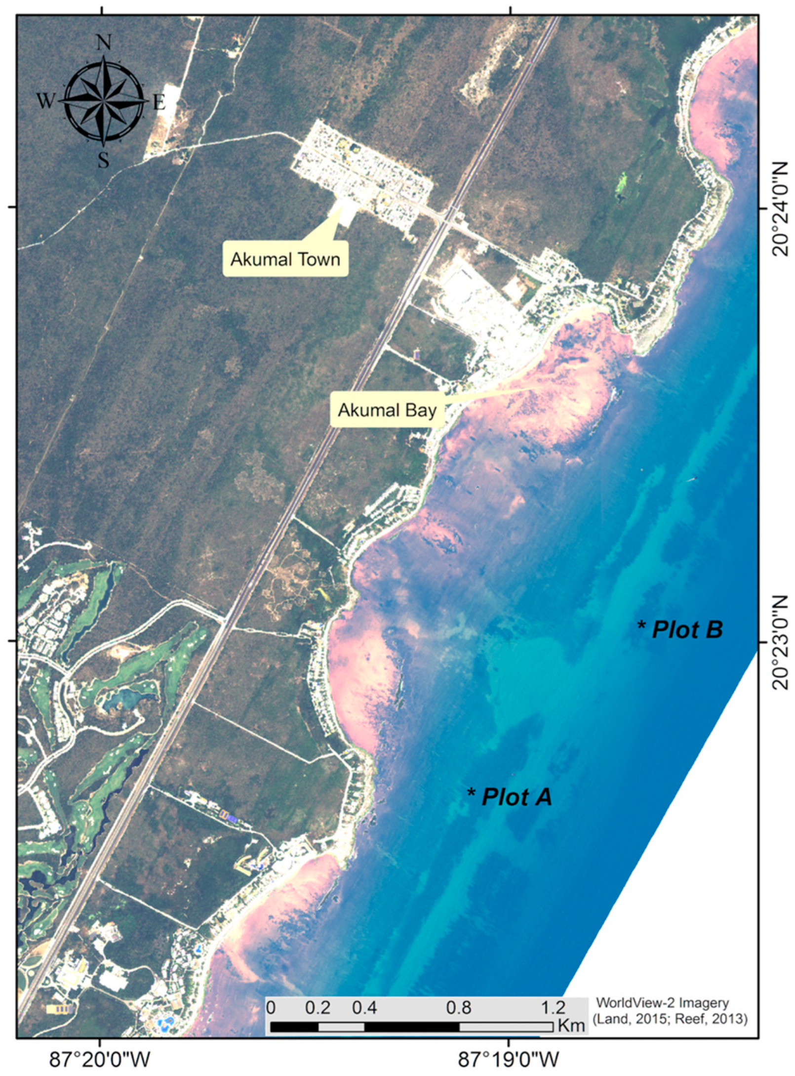
2.1. Study Area

Akumal reef is a well-developed fringing reef off the eastern coast of Quintana Roo, México; It has a shallow reef lagoon with a conspicuous seagrass bed, coral patches, bottoms associated with algal assemblages and coral rubble, and a well-developed back-reef zone which passes into a discontinuous reef crest, that separates the lagoon zone from the reef front. The reef front (4 to 12 m deep) and reef slope zones are well developed, starting on a hard-ground plain at 5–6 m and giving way gradually to tracts of denser colonies that increase in rugosity, that pass into spur and groove areas that end at ~15–16 m by a sand channel, and the reef slope continues with this spurs-and-grooves system at 16–17 m deep, reaching down to 30–35 m deep in a buttress zone (Figure 1).

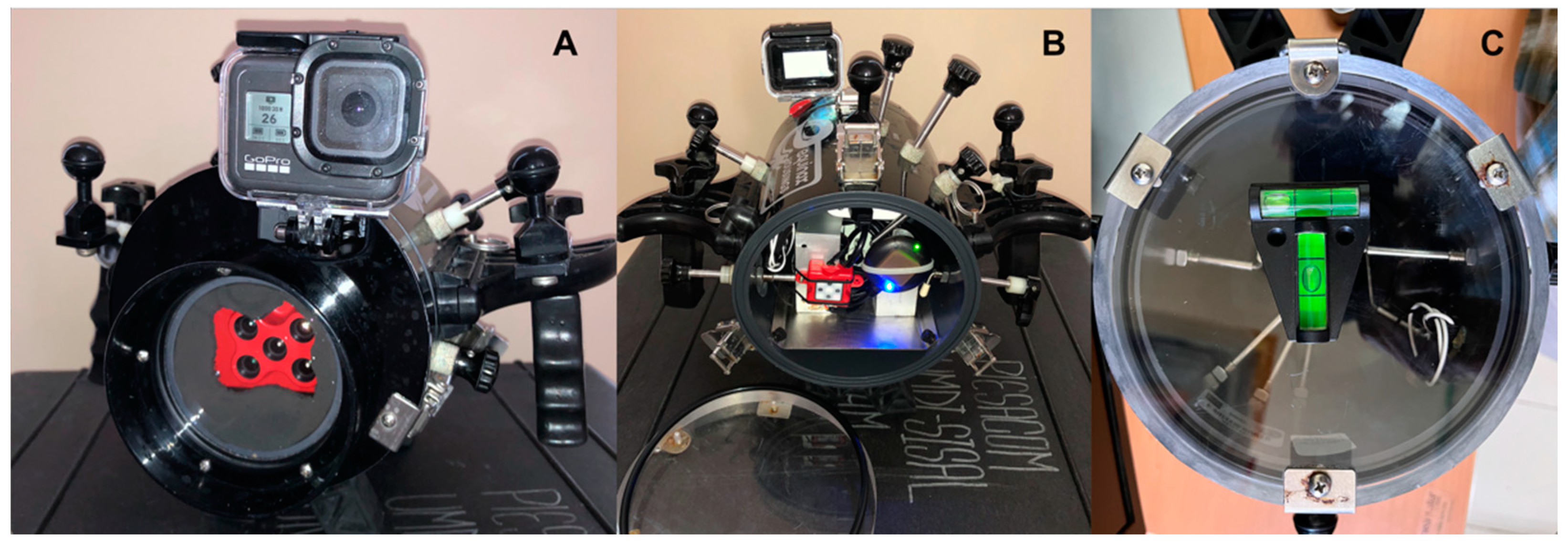
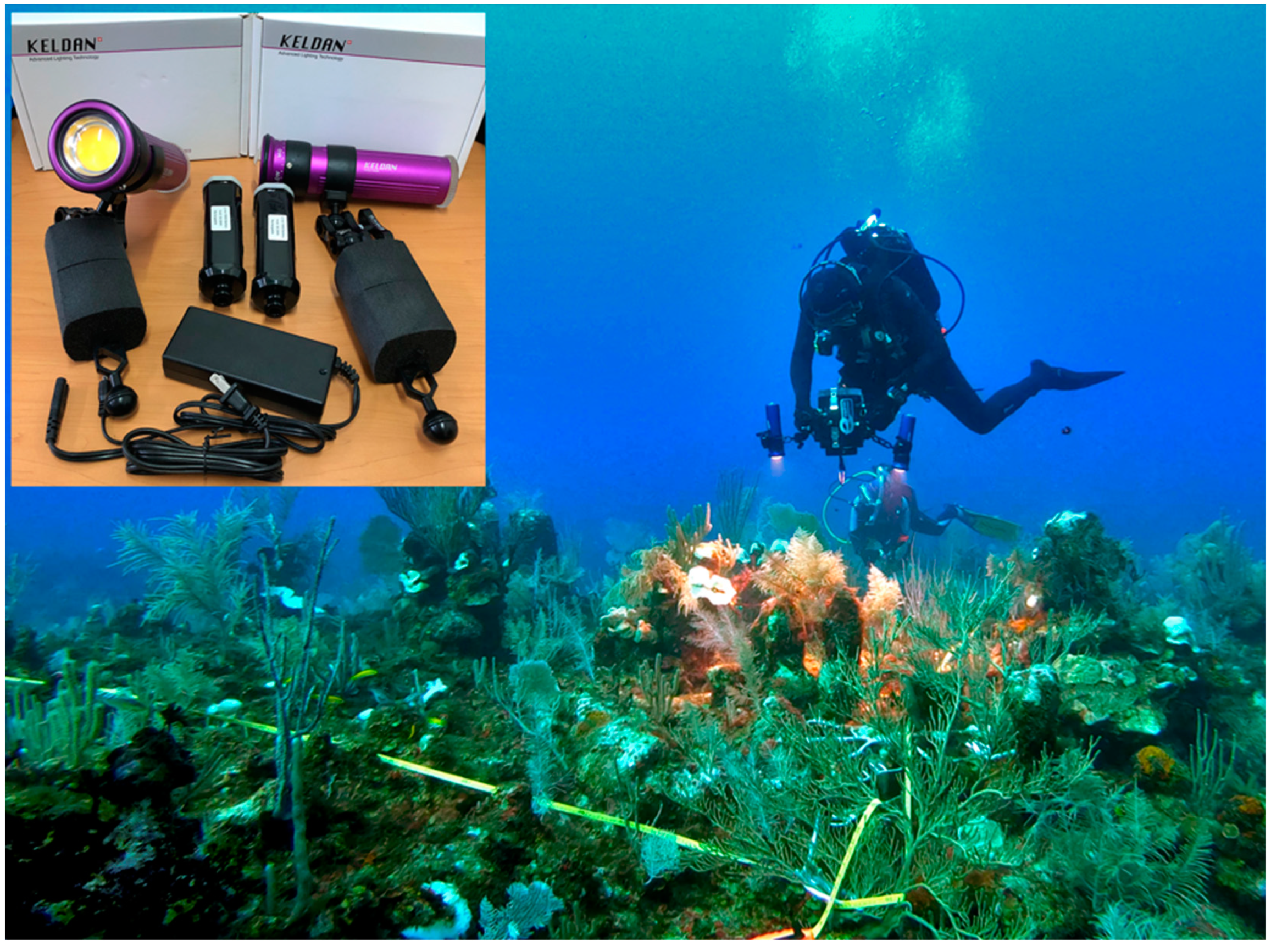
2.2. Field Equipment

Multispectral Sensor: The multispectral sensor employed was a MicaSense^® RedEdge-M camera. This sensor was designed for agricultural assessments hence its five narrow bands: blue, green, red, red edge, and near-infrared (

Table 1. MicaSense RedEdge-M spectral bands specifications [43]. FWHM: full width at half maximum.

Band Number	Band Name	Center Wavelength (nm)	Bandwidth FWHM (nm)
1	Blue	475	20
2	Green	560	20
3	Red	668	10
4	Near IR	840	40
5	Red edge	717	10

) were selected to take advantage of the reflectance of photosynthetic pigments. The RedEdge-M records one image per second on each band at 16-bit radiometric resolution in RAW/TIFF format on an up to 32 Gb SD memory card (writing speed class 10/U3). It has a lens focal length of 5.4 mm and a field of view of 46° [43]). This camera was retrofitted in an acrylic underwater video housing (Equinox, 3D), along with a 10,000 mAh (2.4 A) rechargeable battery (power bank, with USB-A connectivity), along with its GPS antenna and Down Light Sensor (Figure 2A,B).

Depth and Level Monitoring: To maintain a relatively constant height over the substrate a dive computer was attached to the underwater housing, facing the diver; and a two-way (T) level was fixed to the rear plate of the housing (Figure 2C).

A dry (on land) test was performed with the camera system inside the housing to check the appropriate functioning of the sensors (downwelling light sensor, the GPS module, and the multispectral camera). A comparison was carried out using images of the calibration panel captured with the camera outside and inside of the housing, taken at 1 m, under controlled illumination conditions (dark room with two 13,000 lumen lights at full power), to establish if the polycarbonate flat port on the housing had an absorption effect on the light reaching the sensor inside the housing.

Artificial Illumination: To provide a uniform and thorough illumination for the test mentioned above and for the use of the sensor over the reef bottom, we used two LED underwater video lights (Keldan Video 8X) with a maximum output of 13,000 lumen/5600 candelas, a correlated color temperature of 5600° kelvin, a color rendering index (CRI) of 92, and a 110° beam in water. They were mounted to the ball adaptors on the housing handles, using clamps and 20.3 cm (8″) Ultralight arm sections to fix the Keldan lights at ~30 cm to left and to the right from the sensor (Figure 3). Later, a 4-piece kit of StiX adjustable jumbo floats was added to the ultralight arms to enhance the maneuverability and compensate for the buoyancy of the setup.

2.3. Field Tests

Two test sites in Akumal’s reef front were surveyed at different dates and at different depths: Plot A, was a 5 × 5 m plot at −10 m, surveyed during June 2019; and Plot B was a 2.5 × 2.5 m plot at −16.5 m, surveyed in August 2019. The position of the plots was selected because of their diversity in benthic components and bottom types. Plots were delimited by fixing a PVC survey tape to bottom features (rocks or bases of octocorals) on the corners of the plots.

Imagery acquisition was performed with the Micasense RedEdge-M narrow-band sensor, recording images perpendicularly from the bottom, following a grid pattern (left to right, and then front to back) covering the entire plot ensuring high (>50% overlap between images). Before running each photo survey, a small set of images of a calibrated reflectance panel (CRP), originally provided with the sensor, was acquired according to the procedures stated by MicaSense [43]. One set of images was acquired on the boat right before the dive, and one underwater, positioning the panel in the bottom and recording the images at 0.5 m illuminated with both Keldan lights at their maximum power, ensuring the QR code in the CRP appears in the picture. The CRP provided with the camera by MicaSense (RP04-1911069-SC) has the following absolute reflectance values: blue 0.508, green 0.509, blue 0.509, red edge 0.509, and near-infrared 0.507.

Plot A was surveyed at ~1.8 m from the bottom using natural light, under the assumption that the downwelling light sensor (DLS) from the camera would compensate for the light variability during the imagery survey; this plot had large coral colonies, octocorals, and encompassed a deeper section in a sand channel between two spurs. The distance was selected following similar digital photogrammetry approaches [12,14,15,44].

Plot B has a relatively even substrate with small coral and octocoral colonies providing the largest vertical difference in the substrate; it was surveyed applying the same grid pattern as Plot A to acquire imagery for a multispectral orthomosaic, but this time at a 0.5 m height above the substrate using the Keldan lamps at their maximum output.

2.4. Orthomosaic Generation

The imagery datasets acquired at each plot were filtered manually to exclude images not corresponding to perpendicular shots of the reef bottom, not at the specified height or not within the plot areas. They then were processed as follows, using Agisoft MetaShape Pro software v. 1.7 (previously PhotoScan Pro), installed on a PC workstation with Windows 10 Professional (64-bit), dual Intel Xeon processors, 128 GB RAM, dual AMD Radeon FirePro w8100 GPUs, and 2TB HDD:

(1)

A camera calibration file was created for each band of the sensor, following the MetaShape manual [45], and then the parameters in these files were applied to the imported multispectral imagery datasets.

(2)

The reflectance of these multispectral images was calibrated manually using the images of the CRP, and its reflectance values corresponding to each band (included in the CRP).

(3)

The primary channel was set to band 2 (green) since it provides the best visual contrast for these underwater images.

(4)

Metasahape workflow was followed using these settings: Image alignment (highest accuracy, generic preselection, excluding stationary tie points—useful for excluding suspended particles from the alignment process); build dense cloud (quality ultra-high, depth filtering moderate and calculating point confidence), dense cloud filter by confidence (range 0–2); build mesh (source data: dense cloud; surface type: height field; face count: high; interpolation enabled), and build orthomosaic using mesh as surface, and mosaic blending mode, also enabling hole filling.

(5)

The resulting orthomosaics (16-bit) were transformed to normalized reflectance (0–1 value range), creating new bands in the Raster Transform/Raster Calculator tool where bands are divided by the normalization factor of 32,768 [46], and exporting the resulting composite image as TIFF, selecting the index value in the raster transform field.

2.5. Artificial Ilumination Test

The artificial illumination test was performed by acquiring a few sets of images with the narrow-band sensor at different heights (0.5 m, 0.75 m, and 1 m) above the surface of an Orbicella franksi coral colony, using two Keldan Video 8X lamps at their maximum light output, carefully adjusting the position of the beams to light evenly the substrate perpendicular to the sensor. Three orthomosaics of the O. franksi were resolved and 1150 pixels over the coral colony were selected randomly to test the difference among the pixel values per band (R, G, B, RE, NIR) at the three different distances. This test was carried out by applying multivariate analysis (ANOSIM and SIMPER, in the software Primer v6.1.14, Primer-E Ltd., Brugg, Switzerland).

2.6. Orthomosaic Preprocessing

A visual inspection of the orthomosaic from Plot B revealed variability in the pixel values across homogeneous surfaces (salt and pepper effect) due in part to orthomosaic generation artifacts and to the small size of the pixels (Garza-Pérez, Nuñez-Morales and Rioja-Nieto -in prep.-). This impact was addressed by applying a Local Sigma Filter (LSF; 9 × 9 pixels), which preserves fine details and markedly reduces speckle [47], in ENVI v.5.3 (Excelis).

Moreover, during the visual inspections a few orthomosaics, construction artifacts associated to rolling shutter effects were noted, including chromatic aberrations on moving objects (i.e., soft corals), and blurred areas on fixed objects. These artifacts prevented the use of the entire area of the orthomosaic for classification tests, so two smaller areas of the othomosaic (subsets B I and B II), with correctly resolved bottom features, were cropped to test as a proof-of-concept. Later, a mask was applied to remove artifact-ridden areas, and to apply a rigorous supervised classification to the largest possible usable area.

2.7. Supervised Classification

For the initial proof-of-concept visual inspections of the subplots B I and B II defined the different benthic components (classes) in each dataset, classes were trained to digitize 20 fields over positively identified features for each class (n = 20 fields × #of classes). For plot B full, a total of 7993 pixels were used to train the different identified classes, with as few as 325 points for smaller benthic components, and as many as 1100 points for larger benthic components. Class separability was calculated (ROI Tool/ENVI 5.3) for the training fields defined in plots B I, B II, and B full, following the recommendation to edit the shape and location of some fields to increase the calculated separability values closer or above 1.9 on the reported Jeffries–Matusita and transformed divergence separability measures [48].

Several supervised classification methods available on ENVI 5.3 were applied to the three subset plots (B I, B II, and B full), i.e., Mahalanobis distance, maximum likelihood, minimum distance, neural net, and support vector machine, to find the best-classified product. Classified products from subplots B I and B II were assessed first to define if the multispectral orthomosaic was able to accurately separate bottom features. Moreover, for subplot B I, a test was carried out to define the usefulness and discrimination power of an R, G, B band subset vs. the R, G, B, RE. This test used the same training fields coupled with the classification algorithms that produced the most accurate products for the 4-band subset. A post-classification procedure (majority analysis with a 3 × 3 kernel) was applied to all supervised classification products to remove the salt-and-pepper effect and to present more spatially coherent classes.

The accuracy of the supervised classifications was assessed both visually, to compare the results with the spatial patterns of benthic components in the original multispectral orthomosaic, and through the accuracy assessment using overall accuracy, Kappa [49] and Tau [50] coefficients. A stratified random approach to generate points over the different classes in the classified products was used to generate confusion matrices, thus avoiding the spatial correlation bias of using polygons (clusters of pixels) as the ones used to train the classes in subplots B I and B II. A Z-test was applied to the Tau coefficients obtained from the different supervised classification products of Plot B full to assess and objectively select the best one. The next diagram (Figure 4) depicts the methods flowchart.

3. Results

3.1. Field Tests

3.1.1. Sensor Backfitting and Dry-Land Imagery Capture Test

The camera, DLS, and GPS module worked properly when fitted inside the sealed housing. Camera control was responsive using its Wi-Fi connection through a web browser in a mobile device (Apple iPhone X), and GPS was able to acquire all satellites to fix both the geographic location of the camera and the date and time on the captured images. Multispectral images were acquired continuously to test the consistency of the power bank energy output, and the operating autonomy of the setup. The limiting factor for maximum operation time (~45 min) is the SD card memory space, which fills completely in that time, capturing all five bands at 1 s intervals. The powerbank provided consistent power during this period for the camera to operate adequately. The housing flat port test found no significant difference (p = 0.05) between sample values from images acquired inside vs. outside of the housing.

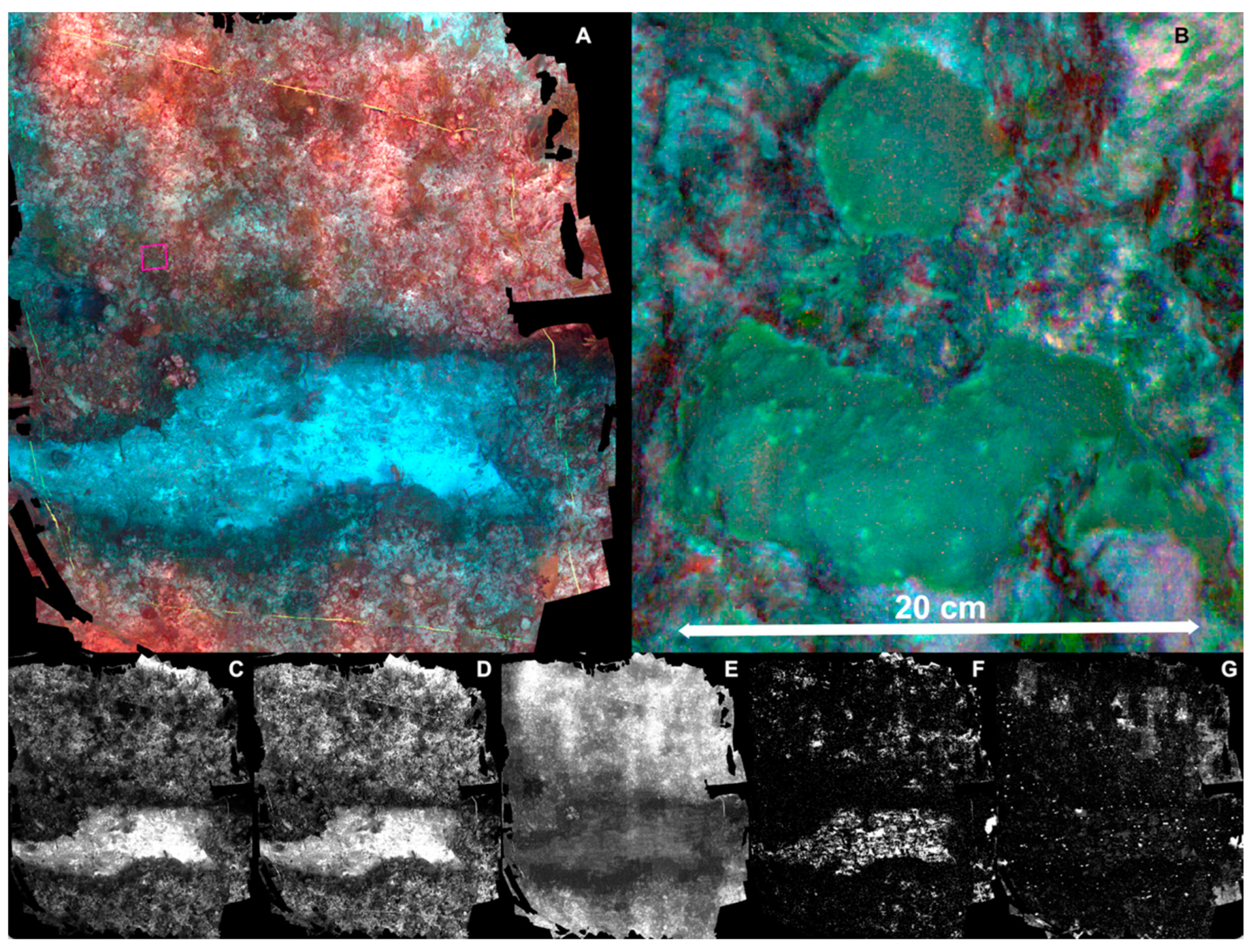
3.1.2. Underwater Orthomosaic Plot A

Plot A was surveyed successfully at a 1.8 m height, and acquired imagery was processed on Agisoft MetashapePro software. The resulting orthomosaic (Figure 5A) was resolved adequately preserving the spatial structure (shapes of benthic components and geomorphology), it has an area of ~25 m² at a spatial resolution of 0.8 × 0.8 mm/pixel. Although this resolution is sufficient to visually identify benthic organisms (Figure 5B) and inert bottom types, it lacked a consistent spectral response along the whole orthomosaic. Banding artifacts are noticeable (light/dark pattern), which the DLS data (used on the orthomosaic generation) was not able to homogenize. Moreover, the distance to the bottom rendered useless both the red edge and NIR bands, whereas the red band had severe shortcomings, and the blue and green bands contained adequate data (Figure 5C–G). After this partial success, and as expected, the need for artificial illumination was established; thus, we performed a test using artificial illumination at different heights above the bottom.

3.1.3. Artificial Lighting Test

Three orthomosaics were resolved for each O. franksi image set at three different distances (0.5 m, 0.75 m, and 1 m). The values of 1150 randomly selected pixels over the coral colony in each orthomosaic were used to test for significant differences among them. The one-way ANOSIM test (using distances as a factor) pointed to the existence of significant differences between the 0.5 m distance group and the 0.75 m and 1 m groups (R = 0.92 for both groups, Global R = 0.561, at a 0.1 significance level), and no significant differences between the 0.75 m and 1 m groups (R = 0.37, 0.1 significance level). This was confirmed with the SIMPER test, which revealed tight groups for pixel values at each distance (average squared distance within groups of 0.4, 0 and 0, for 0.5 m, 0.75 m, and 1 m distances, respectively) with an average squared distance between groups of 0.89 between the 0.5 m group and the 0.75 m and 1 m groups.

The statistically significant differences in pixel values between the 0.5 m dataset and the 0.75 m and 1 m datasets were assessed visually. The closer-distance orthomosaic had better spatial feature definition in all five bands and its pixel values were higher in contrast to the farther datasets (variability charts in Supplementary Materials Figures S1–S5, end member spectral signatures Tables S6 and S7). We established the 0.5 m distance as the option most suitable for capturing useful pictures on all 5 bands and producing orthomosaics with at least 4 useful bands. Thus, we proceeded to survey Plot B at that height, while ensuring the Keldan lights’ beams were correctly pointed to the camera’s field of view, and the lamps set at full power.

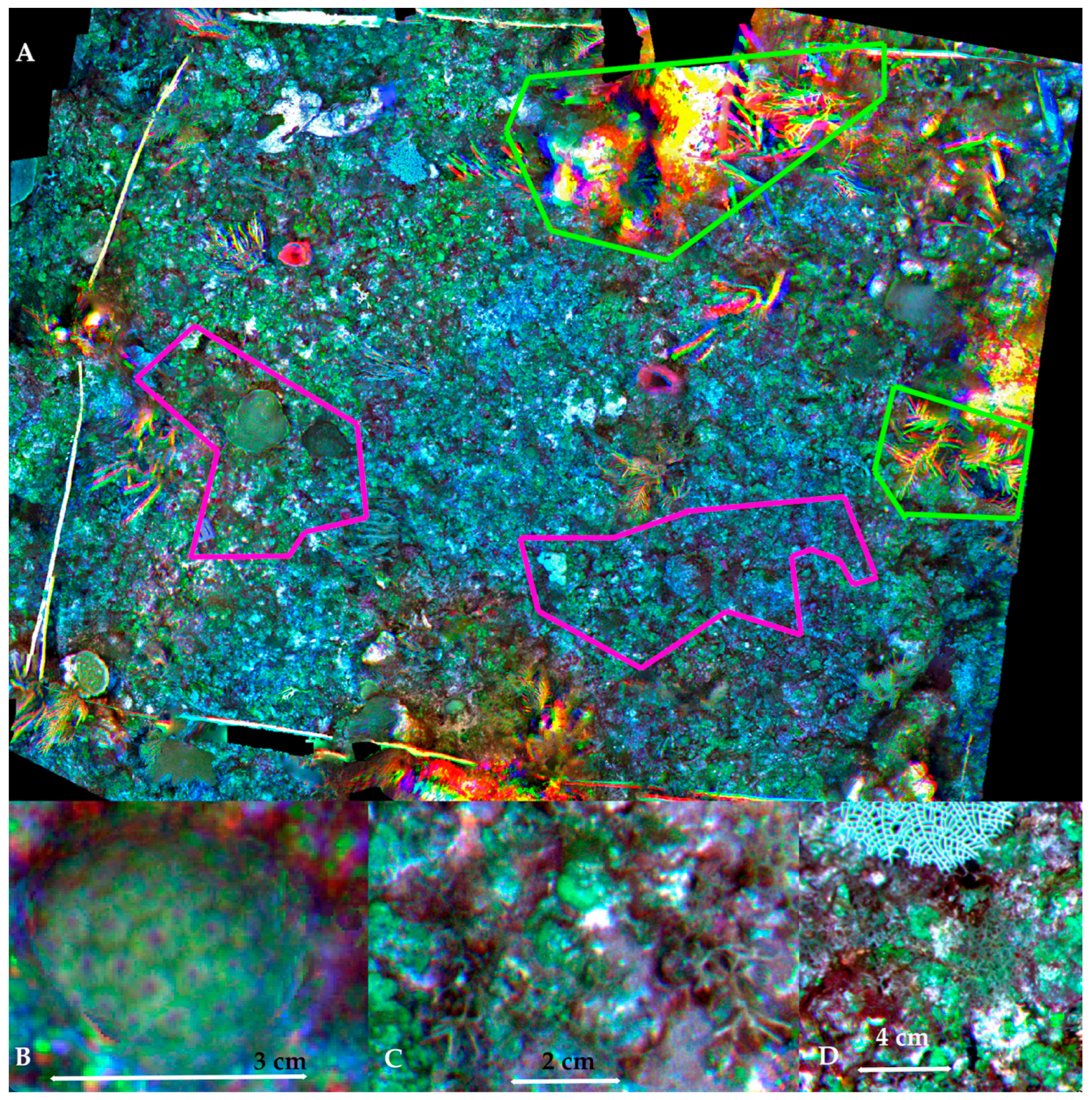
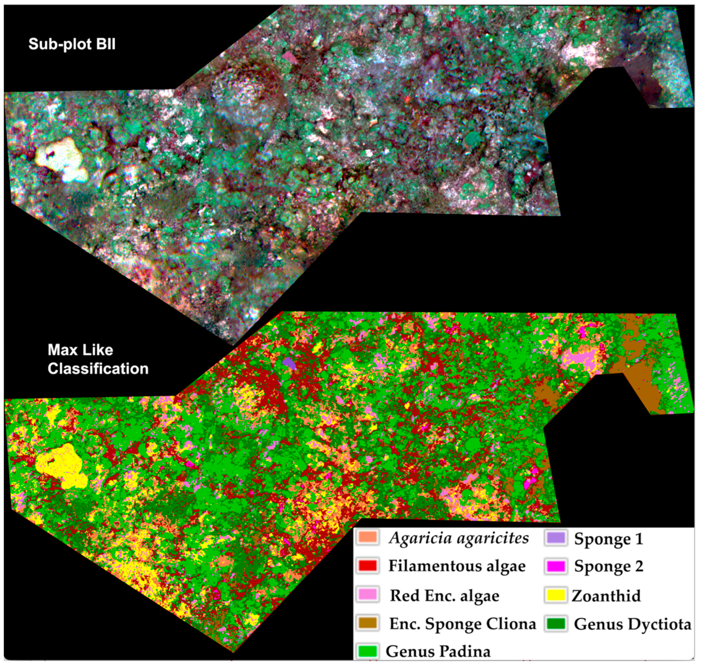
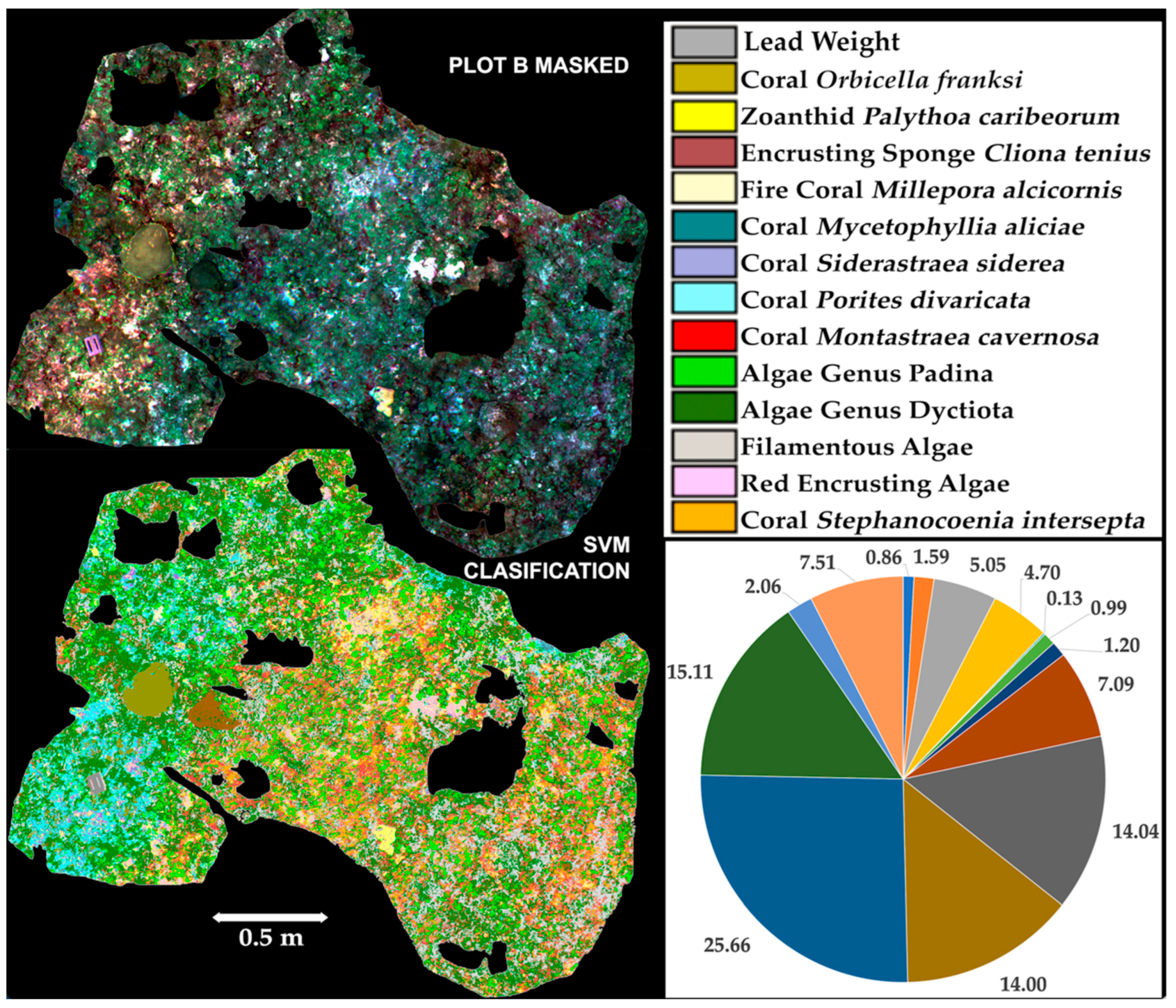
3.1.4. Underwater Orthomosaic Plot B

The resulting orthomosaic from Plot B, surveyed at 0.5 m from the bottom, had a 0.4 × 0.4 mm/pixel spatial resolution, and bands blue, green, red, and red edge contained useful data, whereas data from NIR band, once again, was useless for the purposes of resolving a multispectral band representing accurately the spatial structure of the reef bottom. The spatial structure of the bottom was preserved in most of the orthomosaic, except for (a) moving objects (soft corals that rock to-and-fro due to the water movement of waves or currents); and (b) objects (rocks and coral colonies) that rose markedly above the bottom, thus were much closer to the lens (Figure 6). The moving objects produced chromatic aberrations since the brief delay between bands capture allowed for a difference in the positions of branches amplified by the different position of the lenses, as well as the different position of the diver. Tall objects were not adequately resolved and showed significant distortion (Figure 6, green highlighted areas).

3.2. Supervised Classification

The ultra-high spatial resolution of the resulting orthomosaics facilitates accurate visual identification of benthic organisms, such as hard corals and zoanthids to the species level, types of algae (fleshy brown and red, calcareous green and red, crustose coralline and filamentous algae), morphotypes of sponges and octocorals, as well as inert substrate (sand, rubble, calcareous pavement).

The proof-of-concept for the supervised classification of underwater multispectral orthomosaics included cropping two data subsets from Plot B (B I and B II, Figure 6 pink highlighted areas), where the spatial structure of the bottom was well preserved and there were several bottom components represented. A first attempt used data subsets from the original orthomosaic generated by MetashapePro software (with DN values converted to reflectance), which produced classifications with adequate accuracy (72.56% average overall accuracy; to improve the accuracy of the classifications, a Local Sigma filter (9-pixel radius) was applied to the orthomosaic from which new subsets B I and B II were cropped again.

Twelve different benthos components were visually identified in data subset B I, whereas only nine were identified in subset B II, although for this, there were three additional and different components to those in subset B I (

Table 2. Benthic components identified in subplots B I and B II of the orthomosaic, NP = class not present in subplot.

Class	Classes Plot B I	Classes Plot BII
1	Coral Agaricia agaricites	Coral Agaricia agaricites
2	Coral Orbicella franksi	NP
3	Encrusting Sponge Cliona Tenius	Encrusting Sponge Cliona Tenius
4	Fire Coral Millepora alcicornis	NP
5	Coral Montastraea cavernosa	NP
6	Sponge Callispongia vaginalis	NP
7	Lead weight	NP
8	Algae Genus Dyctiota	Algae Genus Dyctiota
9	Algae Genus Padina	Algae Genus Padina
10	Red Encrusting Algae	Red Encrusting Algae
11	Filamentous Algae	Filamentous Algae
12	Octocoral	NP
13	NP	Encrusting Sponge 1
14	NP	Encrusting Sponge 2
15	NP	Zoanthid Palythoa caribeorum

). Training field separability was calculated using the 20 training fields digitized over each class of benthos components, for each data subset (Supplementary Materials, Tables S1 and S6), and the values were deemed satisfactory. Most of the pairwise comparisons on B I (73% of class pairs) and B II (85% of class pairs) were ≥1.9 on the Jeffries–Matusita and transformed divergence Indexes.

Different supervised classification algorithms were applied to both data subsets using 20 training fields per class. The most accurate supervised classification for B I and B II subsets, preprocessed with the 9-pixel LSF, and post-processed with the majority analysis were produced with the ML algorithm, with an overall accuracy of 84.37%, and 0.83 for Kappa and Tau coefficients for subplot B I (Figure 7), and for B II an overall accuracy of 78.86% and 0.74 for Kappa coefficient and 0.86 for Tau coefficient (Figure 8) (

Table 3. Accuracy assessment values for subplot B I and B II before and after LSF, also compared to Postclassification (Postcl) applying a majority analysis. SCA, supervised classification algorithm; OA, overall accuracy; Kappa, Kappa coefficient; Tau: Tau coefficient; SVM; support vector machine; ML, maximum likelihood; Mh, Mahalanobis.

		Original			LSF 9-Pixels
Subplot	SCA	OA	Kappa	Tau	OA	Kappa	Tau
B I RGBRE 12 classes	SVM	79.00%	0.77	0.77	81.64%	0.79	0.80
	ML	79.86%	0.78	0.78	79.86%	0.78	0.78
	Mh	64.97%	0.61	0.62	67.26%	0.64	0.64
BI RGB	SVM	-	-	-	67.18%	0.63	0.64
12 classes	ML	-	-	-	64.12%	0.60	0.61
B I RGBRE 12 cl/Postcl	SVM	-	-	-	82.97%	0.81	0.81
	ML	-	-	-	84.37%	0.83	0.83
	Mh	-	-	-	69.30%	0.66	0.67
B II RGBRE	ML	70.15%	0.65	0.66	72.29%	0.68	0.68
9 classes	SVM	68.80%	0.64	0.64	70.17%	0.65	0.66
B II RGBRE	ML	-	-	-	78.86%	0.74	0.76
9 c/Postcl	SVM	-	-	-	73.84%	0.69	0.70

, Supplementary Materials Tables S2–S5, S7 and S8).

An additional test compared the supervised classification products of subplot B I with 4-band (R, G, B, RE) vs. its 3-band image subset (R, G, B). Using the same training fields for 12 classes on both images, we applied the two most accurate classification algorithms for the 4-band subset (SVM and ML). Average pair separability (Jeffries–Matusita index) decreased from 1.94 S.D. ± 0.11 for the 4-band image vs. 1.78 S.D. ± 0.33 for the 3-band image. Classification accuracies also decreased for the 3-band subset (Table 3).

The adequate separability of benthic components as well as the accuracy of these classified products, established a basis to attempt the classification of plot B full pre-processed with LSF, removing the poorly resolved areas by masking prior to the supervised classification (Figure 9). A different approach was used to train this masked dataset; in it, 7993 pixels selected manually trained 14 benthic components (classes) (

Table 4. Benthic components (classes) identified in the masked dataset (B Full) of the orthomosaic, and the percentage of cover extracted from the SVM classification.

Class	Name	Cover Percentage (%)
1	Lead weight	0.86
2	Coral Orbicella franksi	1.59
3	Zoanthid Palythoa caribeorum	5.05
4	Encrusting Sponge Cliona tenius	4.70
5	Fire Coral Millepora alcicornis	0.13
6	Coral Mycetophyllia aliciae	0.99
7	Coral Siderastraea siderea	1.20
8	Coral Porites divaricata	7.09
9	Coral Montastraea cavernosa	14.04
10	Algae Genus Padina	14.00
11	Algae Genus Dyctiota	25.66
12	Filamentous Algae	15.11
13	Red Encrusting Algae	2.06
14	Coral Stephanocoenia intersepta	7.51

). The most accurate supervised classification product for Plot B full was generated by the SVM algorithm when applying the majority analysis as post-classification; with an overall accuracy of 82.77%, and Kappa and a Tau coefficients value of 0.81; (

Table 5. Overall accuracy, Kappa and Tau coefficients values obtained from classification with different algorithms of the masked orthomosaic.

Algorithms	Overall Accuracy	Kappa Coefficient	Tau Coefficient
Maximum likelihood	82.46%	0.81	0.81
Neural net	70.40%	0.67	0.68
SVM	82.77%	0.81	0.81

; class separability table and confusion matrix are reported in Supplementary Materials Tables S9 and S10).

The error matrices generated from the three most accurate supervised classifications of Plot B full, using SVM, maximum likelihood, and neural network, were compared by applying a Z-test on the Tau coefficients to test for significant differences among them. Z-values consistently less than 1.96 suggest that there are no significant differences among classification products (

Table 6. Z values obtained for the comparison of error matrices of the masked orthomosaic classifications using the Tau coefficient.

Classification Comparison	Z
Maximum likelihood vs. neural net	0.79
Maximum likelihood vs. SVM	0.022
Neural net vs. SVM	0.90

).

4. Discussion

4.1. RedEdge-M Underwater Operational Limitations

The multispectral orthomosaic from plot A (25 m²) represents the optimal extent surveyable with this kind of setup, since the autonomy of this camera model (RedEdge-M) is limited by the maximum SD memory capacity (32 Gb). This memory size translates into ~45 min of imagery collection, although it is possible to extend this time by turning off the capture of one or more bands, thus using less memory. This scenario would apply in the case of the NIR band which is of limited usefulness according to our results. As a note, new versions of the RedEdge cameras accept larger memory cards (128 Gb) that should allow for a longer autonomy recording images.

Multivariate tests defined the existence of significant differences between the O. franksi dataset acquired at 0.5 m distance and the datasets acquired at 0.75 and 1 m distances. Pixel values were higher on the 0.5 m distance, and visually objects were better represented in comparison with the orthomosaics at other distances. This optimal distance to the substrate of 0.5 m to collect useful data on at least four bands (B, G, R, RE) increases the time needed to survey that area as sweeps are narrower and data require very slow swimming to avoid image blurring. In comparison, other underwater digital photogrammetry approaches acquire pictures at distances ranging from 1 to 2 m above the bottom using camera lenses with similar or wider FOV (47.2° for RedEdge-M vs. 42° to 100° for 55 to 18 mm lenses) [12,14,15,44], allowing the photographic survey of plots up to 100 m² in roughly the same time.

The optimal acquisition of underwater multispectral data with this MicaSense required the use of artificial illumination to balance and rectify the amount of light recorded in each band. This factor reduces the system’s autonomy further, since Keldan lights (Video 8X) have a full-power burn time of ~40 min [51], and other available underwater lights with similar specifications have even shorter burn times (Light & Motion Sola Video 15K, 35–40 min).

4.2. Artificial Illumination

Regarding the need for artificial illumination, in an experiment under controlled laboratory conditions, Guo et al. [38,39] measured light detection with a multispectral sensor at distances up to 2.6 m for blue (420 nm) and yellow (520 nm) bands. Steiner [52] in a gray-literature article mentions that LED light (90-CRI) signal is still detectable up to 2.25 m in clear seawater, although reducing colors close to a monochromatic scale, showing the best color intensity at 0.75 m. Our Plot A was surveyed at a depth of 10 m without artificial illumination, and at a distance of ~1.8 m from the bottom; accordingly, we could still collect useful data on the B (475 nm, center wavelength) and G bands (560 nm, center wavelength).

Our tests on the artificial illumination in the field, on the one hand, empirically showed that there was no visible illumination effect of the two Keldan lights at full power positioned 1.8 m above the substrate. On the other hand, the analysis of the scene-relative reflectance values from the O. franksi colony recorded at different distances found that 1 m and 0.75 m distances provide poor spectral data in bands R, RE, and NIR, and higher scene-reflectance values are obtained for all bands at 0.5 m, but NIR images at even that short distance commonly are of very limited use, specifically because the NIR band resolved in the orthomosaics is mostly blurry noise. The placement of the two Keldan lights to the sides of, and separated from, the sensor (Figure 3) is optimal to reduce backscatter and offers the greatest attenuation length values for this underwater imaging system [53,54].

4.3. Spatial Coherence of Multispectral Orthomosaics

The need for geometric calibration of the RedEdge-M camera has been recognized before [55], and specialized SfM software such as MetaShapePro provides means to carry out this calibration. Although the resulting orthomosaics using this camera lens calibration tool offer better spatial structure accuracy, the difference in the lenses position for each band detector is an unresolved issue, especially for this short-distance approach. The optimal distance of 0.5 m for acquiring useful multispectral data, established after our field tests, produces chromatic aberrations by differences in pixel alignment even in adequately resolved surfaces. These small misalignments do not have a notorious visual impact on the spatial patterns of the supervised classification products, although they should introduce errors in the classification by decreasing the user and producer accuracies. Another issue is non-rigid benthic structures (octocorals, macroalgae canopies above a certain height, wandering fish) that move between image captures, and objects too close to the lens (higher coral colonies) that produce areas in the orthomosaic with poorly resolved features.

4.4. Spectral Accuracy of Multispectral Orthomosaics

Underwater artificial illumination introduces an associated issue, its non-uniform distribution, producing variations with even small changes in the distance from the bottom, given by both the motion of the diver operating the system, and the inherent changes in bottom topography. These variations in the absorption of light in water, driven by differences in distance, were recorded by the different sensor bands, and were conspicuous in some parts of other orthomosaics not used in this study. We assume these variations are also present in plot B and might play a role both in the discrimination of different benthic components, and in the resulting accuracy of the classifications. Visual analysis of the SVM classification of plot B Full, reveals an overestimation of the percent cover of coral P. divaricta, (light blue class in Figure 9), probably due to this non-uniform light distribution.

Although special care was taken to illuminate the substrate with a wide spectrum light and calibrate the reflectance of the orthomosaics using the CRP, reflectance values in the multispectral orthomosaic were neither similar nor comparable with known spectral signatures of reef benthic components (Goodman and Rodríguez Vázquez—unpub. data). Light variability is the key to this incompatibly, since reflectance data were measured using a GER-1500 spectrometer, in an environmental light-sealed contraption using halogen light [56].

The reflectance values in the orthomosaic are quite low. Thus, all spectral information in the orthomosaic is considered scene-relative reflectance, but still useful for the supervised classification of reef benthos components. The examples of the spectral signatures of six different benthic components in Figures S6 and S7 (Supplementary Materials) illustrate this scene-relative reflectance concept. In Figure S6, reflectance values for the 5 bands have completely different scales from the values in Figure S7. The two image sets from where these values were obtained, were collected within 2 min from each other and at relatively the same depth (−16.5 m), at the measured distances of 0.5, 0.75, and 1 m, and the orthomosaics were calibrated with the same CRP image dataset. Nevertheless, the reflectance values of the five benthic components in Figure S7 (three coral species Agaricia agaricites, Stephanocoenia intersepta and Montastraea cavernosa, one brown algae genus—Padina, and red encrusting algae) are higher than the values of O. franksi, which are more in line with the scale of the orthomosaic (plot B) values, but not entirely comparable among them.

4.5. Additional Spectral and Spatial Caveats

At this point, results identify a tradeoff between correctly resolving benthic features and robustly characterizing their spectral signatures. While a greater distance of the multispectral camera to the bottom allows for the correctly resolving benthic components at different heights from the substrate (Plot A, Figure 5), it introduces two important issues: The first is the nullification of the main advantage of artificial illumination—higher scene—relative reflectance values on all bands—due to light attenuation as the signal decreases with distance. The second is the scattering light effect on the bottom features which amplifies the variability of natural illumination (sun light) over the substrate [54,57], given by passing clouds and waves, which at 0.5 m and with the aid of artificial illumination is not visually noticeable, as the field of view of the camera is saturated by the underwater lamps (Figure 3). That increase in the variability of natural light and associated signals from the substrate trumps the assumptions of spectroscopy and optical remote sensing [32,58], causing uneven (darker vs. brighter) spectral responses of the same substrata (Figure 5). The DLS information, in theory, could be used to calibrate this variation, since the sensor is placed towards the back of the housing with the transparent acrylic backplate. Nonetheless, according to the MicaSense knowledge base [59,60,61], the use of these DLS data is advisable only with totally overcast conditions, and not in the rapidly shifting situation mentioned above. In future applications of this method, it could be useful to implement corrections algorithms such as the one proposed by Gracias et al. [62] to remove sunlight flicker for orthomosaics at higher distances.

4.6. Multispectral Orthomosaic Classification Accuracy and Implications

Usually, as pointed out by Andrefoüet et al. [18], supervised classification accuracy decreases inversely to the number of classes and the heterogeneity or complexity of the habitat, i.e., A decrease of 12% in overall accuracy from schemes of 4–5 classes to schemes of 9–11 classes. For our products, even with the pixel misalignment issue, the supervised classifications of B I and B II had a high accuracy for 12 and 9 classes, respectively (up to 84.37% overall accuracy, and 0.83 for Kappa and Tau coefficients), with the capability of discrimination between objects of very similar spectral signatures, such as different coral species in subplot B I (Agaricia agricites vs. Montastraea cavernosa, and Orbicella franksi vs. Montastraea cavernosa with separation values of 1.97 and 1.98 in the Jeffries–Matusita index respectively), and also between different genus of brown algae in subplot B II (Genus Padina vs. Dyctiota with 1.91 separation in the Jeffries–Matusita index), along with the discrimination between other common substrates as filamentous algae, red encrusting algae, sponges, zoanthids and octocorals. The reported accuracy by Gleason et al. [3] for supervised classification of multispectral images using 9 to 12 classes, ranges from 70 to 75% and is comparable with the accuracies obtained in this study.

A preprocessing of the multispectral orthomosaics—even as simple as the Local Sigma Filter—to despeckle ultra-high spatial resolution products consistently helps to enhance the accuracy of the supervised classifications. This accuracy enhancement can be up to 2.64% for overall accuracy, and Kappa and Tau coefficients can improve up to 0.2 depending on the accuracy of the original products; lower accuracy products generally benefit more from this preprocessing than the products with higher accuracies. Post-processing (majority analysis) of the supervised classification products systematically enhanced their accuracy, from a modest 0.6% to a 6.5% in overall accuracy, and 0.1 to 0.6 in Kappa and Tau coefficients values (Table 3).

These encouraging results led to the classification of full plot B, masking out the poorly resolved areas; these classifications in general had similar accuracy (up to 82.77% overall, 0.81 Kappa and Tau coefficients) to the subplots B I and II, but this time using a classification scheme of 14 benthic components. The comparison (Z-test) between the Tau coefficients of the classified products did not show statistically significant differences, so we kept our choice of the SVM classification for the estimation of the percent cover of coral benthos components.

Complex spatial patterns of benthic components, such as the ones observed in these subplots where filamentous algae are mixed with brown and red encrusting algae, make the need for accurate classification approaches (supervised, as well as other pixel and texture-based methods) of paramount importance to the efficient estimation of their cover. Hard coral species such as O. franksi, M. cavernosa, and A. agricites, as well as brown macroalgae Genus Padina and Dyctiota, constitute ecologically important benthic components because of their role as reef condition indicators if converted to a percentage of cover of hard coral and macroalgae [63]. As such, the relevance of their user accuracy values, up to 84.37%, on plots BI and B II validates the possible application of this kind of multispectral products to assess and monitor the condition of coral reefs.

4.7. Comparison with Hyperspectral Approaches

Underwater remote sensing approaches using hyperspectral imaging systems to characterize and classify benthic components [34,36,64] are at least one order of magnitude more expensive (USD + 10 K vs. USD + 100 K), and data are much more complicated to process. This complex data analysis arises from the magnitude of data associated with hundreds of hyperspectral bands and to the number of corrections required to obtain products with adequate spatial geometry; these corrections are needed to measure accurate areas (percentage cover of benthic components). Chennu et al. [34], present a supervised classification of 11 benthic categories, using most of the hyperspectral bands (excluding the NIR portion as in our case), with an average producer accuracy of 95.7% using an SVM algorithm. In comparison, our SVM average producer accuracy for the 14 classes on plot B full was 78.9%. Their approach to supervised classification of an RGB dataset yielded 56.5% in producer accuracy on the same 11 categories vs. our 64.6% on 12 classes for the RGB subset of B I. Although a direct comparison is not possible due to their approach to RGB using narrower bands than the RedEdge-M’s: the blue (460 nm), green (540 nm), and red (640 nm) wavelengths bands, which probably offer too little spectral information.

These comparisons between hyperspectral and multispectral approaches to supervised classification of coral reef benthic components provide the following insights. The hyperspectral datasets have greater discriminant power because of the sheer amount of relevant data, but the multispectral dataset from the RedEdge-M using narrow bands R, G, B, RE, do have an adequate discriminant power, higher than the R, G, B datasets (both by MicaSense and by the hyperspectral sensor), thus highlighting the usefulness of RE band for this purpose. As a note, with all the caveats pertaining to the scene-relative reflectance, Figure S7 (Supplementary Materials) shows a higher response of the five spectral signatures in the RE band, than in the other four bands.

The artificial illumination used on [36] (Keldan Video 8M) is quite similar to our Keldan Video 8X, enabling their hyperspectral sensor to record spectral data at 700 nm, at distances ranging from 06 to 1.8 m. The RedEdge-M’s RE band FWHM comprises the 712–723 nm range, and the spectral power distribution curve of the lights reported in [51] reaches at least 730 nm, although as mentioned above, in our case the distance to the substrate is a limitative factor for acquiring adequate data on this band.

On the spectral ranges identified in earlier studies to discriminate reef benthos, the spectral band center proposed by Hochberg and Atkinson [65,66] in the blue region, and the spectral bands proposed by Holden and LeDrew [33] for green and red regions roughly correspond to RedEdge-M’s B, G and R bands center wavelength and FWHM. These long-accepted spectral bands together with the RE band constitute a powerful set for the classification of coral reef benthic components, reaffirming the usefulness of the proposal by Gleason et al. [3] for using (10 nm) narrow bands (10 and 20 nm in the case of RedEdge-M) for this purpose.

4.8. What Can Be Learned from Other Digital Photogrammetry Approaches?

Other underwater digital photogrammetry approaches exist. Some require digitizing features by hand [14,15] which is time consuming, in addition to the time needed to resolve the orthomosaics, and in some cases digitizing becomes difficult and results could have observer bias on areas where different algae types, or algae types and substrata, are mixed. Advancement in imagery analysis with very high accuracy and tending to the automatization of features identification and mapping, as the semantic mapping [16,64], and the segmentation of orthoprojections [67] are promising approaches that probably constitute the next steps for the analysis of multispectral orthomosaics.

5. Conclusions

A novel approach of using an agricultural multispectral sensor originally developed to be used on unmanned aerial vehicles is applied to the underwater assessment of reef benthic features. This approach had its origins in earlier studies suggesting the use of narrow-band sensors for this purpose, and on the advancement in digital orthomosaics development. As expected, the spectral information produced by the narrow bands (B, G, R, and RE) of the MicaSense RedEdge-M allows for the accurate discrimination of benthic components. One advantage of this approach is the use of the RE band, not present in other underwater digital photogrammetry approaches (e.g., using only RGB sensors), which enhances the discrimination of benthic components and could be used in future studies (pigment content, coral colony health, macroalgae biomass, etc.). The supervised classification of underwater multispectral orthomosaics successfully discriminated most of the coral species present in the area, as well as different types of algae, sponges and zoanthids. This task, however, has its own challenges, including the lack of specialized hardware, as our prototype system had to be adapted to an old video housing, and quality artificial underwater lights of sufficient power had to be added. There is also the issue with the tradeoff between spatially resolving all the benthic features adequately, and obtaining useful data among spectral bands, as the optimal distance from the substrate for the latter is about one-third of the optimal distance for the former. Nevertheless, our proof-of-concept study demonstrates a promising route to a larger-scale and accurate approach to reef benthos mapping, especially in light of the advancement and technological improvements in both multispectral sensors technology and image processing methods.

References

- Hedley, J.D.; Roelfsema, C.M.; Chollett, I.; Harborne, A.R.; Heron, S.F.; Weeks, S.; Skirving, W.J.; Strong, A.E.; Eakin, C.M.; Christensen, T.R.L.; et al. Remote Sensing of Coral Reefs for Monitoring and Management: A Review. Remote Sens. 2016, 8, 118. [Google Scholar] [CrossRef]
- Lang, J.C. Status of Coral Reefs in the Western Atlantic: Results of Initial Surveys, Atlantic and Gulf Rapid Reef Assessment (Agrra) Program. Atoll Res. Bull. 2003, 496. [Google Scholar] [CrossRef]
- Gleason, A.C.R.; Reid, R.P.; Voss, K.J. Automated classification of underwater multispectral imagery for coral reef monitoring. In Proceedings of the OCEANS 2007, Vancouver, BC, Canada, 29 Septerber–4 October 2007; pp. 1–8. [Google Scholar] [CrossRef]
- Gleason, A.C.R.; Gracias, N.; Lirman, D.; Gintert, B.E.; Smith, T.B.; Dick, M.C.; Reid, R.P. Landscape video mosaic from a mesophotic coral reef. Coral Reefs 2009, 29, 253. [Google Scholar] [CrossRef]
- Lirman, D.; Gracias, N.; Gintert, B.E.; Gleason, A.C.R.; Reid, R.P.; Negahdaripour, S.; Kramer, P. Development and application of a video-mosaic survey technology to document the status of coral reef communities. Environ. Monit. Assess. 2006, 125, 59–73. [Google Scholar] [CrossRef]
- Gintert, B.; Gracias, N.; Gleason, A.; Lirman, D.; Dick, M.; Kramer, P.; Reid, P.R. Second-Generation Landscape Mosaics of Coral. In Proceedings of the 11th International Coral Reef Symposium, Fort Lauderdale, FL, USA, 7–11 July 2008; pp. 577–581. [Google Scholar]
- Gintert, B.; Gracias, N.; Gleason, A.; Lirman, D.; Dick, M.; Kramer, P.; Reid, P.R. Third-Generation Underwater Landscape Mosaics for Coral Reef Mapping and Monitoring. In Proceedings of the 12th International Coral Reef Symposium, Cairns, Australia, 9–13 July 2012. 5A Remote Sensing of Reef Environments. [Google Scholar]
- Lirman, D.; Gracias, N.; Gintert, B.; Gleason, A.; Deangelo, G.; Dick, M.; Martinez, E.; Reid, P.R. Damage and recovery assessment of vessel grounding injuries on coral reef habitats by use of georeferenced landscape video mosaics. Limn. Oceanogr. Methods 2010, 8, 88–97. [Google Scholar] [CrossRef]
- Gleason, A.; Lirman, D.; Gracias, N.; Moore TGriffin, S.; Gonzalez, M.; Gintert, B. Damage Assessment of Vessel Grounding Injuries on Coral Reef Habitats Using Underwater Landscape Mosaics. In Proceedings of the 63rd Gulf and Caribbean Fisheries Institute, San Juan, Puerto Rico, 1–5 November 2010; pp. 125–129. [Google Scholar]
- Shihavuddin, A.; Gracias, N.; Garcia, R.; Gleason, A.C.R.; Gintert, B. Image-Based Coral Reef Classification and Thematic Mapping. Remote Sens. 2013, 5, 1809–1841. [Google Scholar] [CrossRef]
- Figueira, W.; Ferrari, R.; Weatherby, E.; Porter, A.; Hawes, S.; Byrne, M. Accuracy and Precision of Habitat Structural Complexity Metrics Derived from Underwater Photogrammetry. Remote Sens. 2015, 7, 16883–16900. [Google Scholar] [CrossRef]
- Edwards, C.B.; Eynaud, Y.; Williams, G.J.; Pedersen, N.E.; Zgliczynski, B.J.; Gleason, A.C.R.; Smith, J.E.; Sandin, S.A. Large-area imaging reveals biologically driven non-random spatial patterns of corals at a remote reef. Coral Reefs 2017, 36, 1291–1305. [Google Scholar] [CrossRef]
- Ferrari, R.; Lachs, L.; Pygas, D.R.; Humanes, A.; Sommer, B.; Figueira, W.F.; Edwards, A.J.; Bythell, J.C.; Guest, J.R. Photogrammetry as a tool to improve ecosystem restoration. Trends Ecol. Evol. 2021, 36, 1093–1101. [Google Scholar] [CrossRef]
- Hernández-Landa, R.C.; Barrera-Falcon, E.; Rioja-Nieto, R. Size-frequency distribution of coral assemblages in insular shallow reefs of the Mexican Caribbean using underwater photogrammetry. PeerJ 2020, 8, e8957. [Google Scholar] [CrossRef]
- Barrera-Falcon, E.; Rioja-Nieto, R.; Hernández-Landa, R.C.; Torres-Irineo, E. Comparison of Standard Caribbean Coral Reef Monitoring Protocols and Underwater Digital Photogrammetry to Characterize Hard Coral Species Composition, Abundance and Cover. Front. Mar. Sci. 2021, 8, 722569. [Google Scholar] [CrossRef]
- Yuval, M.; Alonso, I.; Eyal, G.; Tchernov, D.; Loya, Y.; Murillo, A.C.; Treibitz, T. Repeatable Semantic Reef-Mapping through Photogrammetry and Label-Augmentation. Remote Sens. 2022, 13, 659. [Google Scholar] [CrossRef]
- Mumby, P.J.; Green, E.P.; Edwards, A.J.; Clark, C.D. Coral reef habitat-mapping: How much detail can remote sensing provide? Mar. Biol. 1997, 130, 193–202. [Google Scholar] [CrossRef]
- Andréfoüet, S.; Kramer, P.; Torres-Pulliza, D.; Joyce, K.E.; Hochberg, E.J.; Garza-Perez, R.; Mumby, P.J.; Riegl, B.; Yamano, H.; White, W.H.; et al. Multi-sites evaluation of IKONOS data for classification of tropical coral reef environments. Remote Sens. Environ. 2003, 88, 128–143. [Google Scholar] [CrossRef]
- Stumpf, R.; Holderied, K.; Sinclair, M. Determination of water depth with high resolution satellite image over variable bottom types. Limnol Oceanogr. 2003, 48, 547–556. [Google Scholar] [CrossRef]
- Mellin, C.; Andréfouët, S.; Ponton, D. Spatial predictability of juvenile fish species richness and abundance in a coral reef environment. Coral Reefs 2007, 26, 895–907. [Google Scholar] [CrossRef]
- Pittman, S.J.; Christensen, J.D.; Caldow, C.; Menza, C.; Monaco, M.E. Predictive mapping of fish species richness across shallow-water seascapes in the Caribbean. Ecol. Model. 2007, 204, 9–21. [Google Scholar] [CrossRef]
- Hogrefe, K.R.; Wright, D.J.; Hochberg, E. Derivation and Integration of Shallow-Water Bathymetry: Implications for Coastal Terrain Modeling and Subsequent Analyses. Mar. Geodesy 2008, 31, 299–317. [Google Scholar] [CrossRef]
- Knudby, A.; LeDrew, E.; Brenning, A. Predictive mapping of reef fish species richness, diversity and biomass in Zanzibar using IKONOS imagery and machine-learning techniques. Remote Sens. Environ. 2010, 114, 1230–1241. [Google Scholar] [CrossRef]
- Knudby, A.; Roelfsema, C.; Lyons, M.; Phinn, S.; Jupiter, S. Mapping fish community variables by integrating field and satellite data, object-based image analysis and modeling in a traditional Fijian fisheries management area. Remote Sens. 2011, 3, 460–483. [Google Scholar] [CrossRef]
- Hedley, J.D.; Harborne, A.R.; Mumby, P.J. Simple and robust removal of sun glint for mapping shallow water benthos. Int. J. Remote Sens. 2005, 26, 2107–2112. [Google Scholar] [CrossRef]
- Kay, S.; Hedley, J.D.; Lavender, S. Sun Glint Correction of High and Low Spatial Resolution Images of Aquatic Scenes: A Review of Methods for Visible and Near-Infrared Wavelengths. Remote Sens. 2009, 1, 697–730. [Google Scholar] [CrossRef]
- Lyzenga, D.R. Passive remote sensing techniques for map- ping water depth and bottom features. Appl. Opt. 1978, 17, 379–383. [Google Scholar] [CrossRef]
- Lyzenga, D.R. Remote sensing of bottom reflectance and water attenuation parameters in shallow water using aircraft and Landsat data. Int. J. Remote Sens. 1981, 2, 71–82. [Google Scholar] [CrossRef]
- Lyzenga, D.R. Shallow-water bathymetry using combined lidar and passive multispectral scanner data. Int. J. Remote Sens. 1985, 6, 115–125. [Google Scholar] [CrossRef]
- Maritorena, S. Remote sensing of the water attenuation in coral reefs: A case study in French Polynesia. Int. J. Remote Sens. 1996, 17, 155–166. [Google Scholar] [CrossRef]
- Mumby, P.; Clark, C.; Green, E.P.; Edwards, A.J. Benefits of water column correction and contextual editing for mapping coral reefs. Int. J. Remote Sens. 1998, 19, 203–210. [Google Scholar] [CrossRef]
- Goodman, J.A.; Purkis, S.J.; Phinn, S.R. Coral Reef Remote Sensing; Springer: Berlin/Heidelberg, Germany, 2013. [Google Scholar] [CrossRef]
- Holden, H.; LeDrew, E. Hyperspectral identification of coral reef features. Int. J. Remote Sens. 1999, 20, 2545–2563. [Google Scholar] [CrossRef]
- Chennu, A.; Färber, P.; De’Ath, G.; De Beer, D.; Fabricius, K.E. A diver-operated hyperspectral imaging and topographic surveying system for automated mapping of benthic habitats. Sci. Rep. 2017, 7, 7122. [Google Scholar] [CrossRef]
- Kutser, T.; Hedley, J.; Giardino, C.; Roelfsema, C.; Brando, V.E. Remote sensing of shallow waters—A 50 year retrospective and future directions. Remote Sens. Environ. 2020, 240, 111619. [Google Scholar] [CrossRef]
- Summers, N.; Johnsen, G.; Mogstad, A.; Løvås, H.; Fragoso, G.; Berge, J. Underwater Hyperspectral Imaging of Arctic Macroalgal Habitats during the Polar Night Using a Novel Mini-ROV-UHI Portable System. Remote Sens. 2022, 14, 1325. [Google Scholar] [CrossRef]
- Hochberg, E.J.; Atkinson, M.J.; Apprill, A. Spectral reflectance of coral. Coral Reefs 2003, 23, 84–95. [Google Scholar] [CrossRef]
- Guo, Y.; Liu, H.; Chen, Y.; Riaz, W.; Yang, P.; Song, H.; Shen, Y.; Zhan, S.; Huang, H.; Wang, H.; et al. Color restoration method for underwater objects based on multispectral images. In OCEANS 2016—Shanghai; IEEE: Piscataway, NJ, USA, 2016. [Google Scholar]
- Guo, Y.; Song, H.; Liu, H.; Wei, H.; Yang, P.; Zhan, S.; Wang, H.; Huang, H.; Liao, N.; Mu, Q.; et al. Model-based restoration of underwater spectral images captured with narrowband filters. Opt. Express 2016, 24, 13101–13120. [Google Scholar] [CrossRef]
- Yang, P.; Guo, Y.; Wei, H.; Dan, S.; Song, H.; Zhang, Y.; Wu, C.; Shentu, Y.; Liu, H.; Huang, H.; et al. Method for spectral restoration of underwater images: Theory and application. Infrared Laser Eng. 2017, 45, 323001. [Google Scholar] [CrossRef]
- Wei, H.; Guo, Y.; Yang, P.; Song, H.; Liu, H.; Zhang, Y. Underwater multispectral imaging: The influences of color filters on the estimation of underwater light attenuation. In OCEANS 2017—Aberdeen; IEEE: Piscataway, NJ, USA, 2017. [Google Scholar]
- Wu, C.; Shentu, Y.C.; Wu, C.; Guo, Y.; Zhang, Y.; Wei, H.; Yang, P.; Huang, H.; Song, H. Development of an underwater multispectral imaging system based on narrowband color filters. In OCEANS 2018 MTS/IEEE Charleston; IEEE: Piscataway, NJ, USA, 2018. [Google Scholar]
- MicaSense. MicaSense RedEdge-M Multispectral Camera, User Manual Rev 0.1, 47 pag. 2017. Available online: https://support.micasense.com/hc/en-us/articles/215261448-RedEdge-User-Manual-PDF-Legacy (accessed on 30 October 2022).
- Pedersen, N.E.; Edwards, C.B.; Eynaud, Y.; Gleason, A.C.R.; Smith, J.E.; Sandin, S.A. The influence of habitat and adults on the spatial distribution of juvenile corals. Ecography 2019, 42, 1703–1713. [Google Scholar] [CrossRef]
- Agisoft. Agisoft Metashape User Manual Professional Edition, Version 1.7, 179 pag. 2022. Available online: https://www.agisoft.com/pdf/metashape_1_7_en.pdf (accessed on 30 October 2022).
- Agisoft. MicaSense RedEdge MX Processing Workflow (Including Reflectance Calibration) in Agisoft Metashape Professional. 2022. Available online: https://agisoft.freshdesk.com/support/solutions/articles/31000148780-micasense-rededge-mx-processing-workflow-including-reflectance-calibration-in-agisoft-metashape-pro (accessed on 30 October 2022).
- Eliason, E.M.; McEwen, A.S. Adaptive Box Filters for Removal of Random Noise from Digital Images. Photogramm. Eng. Remote Sens. 1990, 56, 453. [Google Scholar]
- Exelis. ENVI-Help, ROI Separability, Exelis Visual Information Solutions. 2015. Available online: https://www.l3harrisgeospatial.com/docs/regionofinteresttool.html#ROISeparability (accessed on 30 October 2022).
- Congalton, R.S. A Review of Assessing the Accuracy of Classifications of Remotely Sensed Data. Remote Sens. Environ. 1991, 37, 35–46. [Google Scholar] [CrossRef]
- Ma, Z.K.; Redmond, R.L. Tau-coefficients for accuracy assessment of classification of remote-sensing data. Photogramm. Eng. Remote Sens. 1995, 61, 435–439. [Google Scholar]
- Keldan. Underwater Video Light VIDEO 8X 13000lm CRI92 Operating Instructions. Keldan Gmbh Switzerland. 2017. Available online: https://keldanlights.com/cms/upload/_products/Compact_Lights/Video_8X_13000lm_CRI92/pdf/Video8X_13000lm_CRI92_Operating_Instructions_english.pdf (accessed on 30 October 2022).
- Steiner, A. Understanding the Basics of Underwater Lighting, Ocean News. 2013. Available online: https://www.deepsea.com/understanding-the-basics-of-underwater-lighting/ (accessed on 1 October 2022).
- Jaffe, J.S. Computer modeling and the design of optimal underwater Imaging Systems. IEEE J. Ocean. Eng. 1990, 15, 2. [Google Scholar] [CrossRef]
- Jaffe, J.S.; Moore, K.D.; McLean, J.; Strand, M.P. Underwater optical imaging: Status and prospects. Oceanography 2001, 3, 64–75. [Google Scholar] [CrossRef]
- Frontera, F.; Smith, M.J.; Marsh, S. Preliminary investigation into the geometric calibration of the micasense rededge-m multispectral camera. Int. Arch. Photogramm. Remote Sens. Spat. Inf. Sci. 2020, XLIII-B2-2020, 17–22. [Google Scholar] [CrossRef]
- Lucas, M.Q.; Goodman, J. Linking Coral Reef Remote Sensing and Field Ecology: It’s a Matter of Scale. J. Mar. Sci. Eng. 2014, 3, 1–20. [Google Scholar] [CrossRef]
- Duntley, S.Q. Light in the Sea. J. Opt. Soc. Am. 1963, 53, 214–233. [Google Scholar] [CrossRef]
- Green, E.P.; Mumby, P.J.; Edwards, A.J.; Clark, C.D. Remote Sensing Handbook for Tropical Coastal Management. In Coastal Management Sourcebooks 3; Edwards, A.J., Ed.; UNESCO: Paris, France, 2000; 316p. [Google Scholar]
- MicaSense. Knowledge Base “What does RedEdge’s Downwelling Light Sensor (DLS) Do for My Data?”. 2022. Available online: https://support.micasense.com/hc/en-us/articles/219901327-What-does-RedEdge-s-Downwelling-Light-Sensor-DLS-do-for-my-data- (accessed on 23 September 2022).
- MicaSense. Knowledge Base “Downwelling Light Sensor (DLS) Basics”. 2022. Available online: https://support.micasense.com/hc/en-us/articles/115002782008-Downwelling-Light-Sensor-DLS-Basics (accessed on 23 September 2022).
- MicaSense. Knowledge Base “Using Panels and/or DLS in Post-Processing”. 2022. Available online: https://support.micasense.com/hc/en-us/articles/360025336894-Using-Panels-and-or-DLS-in-Post-Processing (accessed on 23 September 2022).
- Gracias, N.; Negahdaripour, S.; Neumann, L.; Prados, R.; Garcia, R. A motion compensated filtering approach to remove sunlight flicker in shallow water images. In OCEANS 2008; IEEE: Piscataway, NJ, USA, 2018. [Google Scholar]
- Healthy Reefs Initiative. 2022. Available online: https://www.healthyreefs.org/cms/healthy-reef-indicators/ (accessed on 30 October 2022).
- Rashid, A.R.; Chennu, A. A Trillion Coral Reef Colors: Deeply Annotated Underwater Hyperspectral Images for Automated Classification and Habitat Mapping. Data 2020, 5, 19. [Google Scholar] [CrossRef]
- Hochberg, E.J.; Atkinson, M.J. Spectral discrimination of coral reef benthic communities. Coral Reefs 2000, 19, 164–171. [Google Scholar] [CrossRef]
- Hochberg, E.J.; Atkinson, M.J. Capabilities of remote sensors to classify coral, algae, and sand as pure and mixed spectra. Remote Sens. Environ. 2003, 85, 174–189. [Google Scholar] [CrossRef]
- Runyan, H.; Petrovic, V.; Edwards, C.B.; Pedersen, N.; Alcantar, E.; Kuester, F.; Sandin, S.A. Automated 2D, 2.5D, and 3D Segmentation of Coral Reef Pointclouds and Orthoprojections. Front. Robot. AI 2022, 9, 884317. [Google Scholar] [CrossRef]