Abstract
Sea ice leads, or fractures account for a small proportion of the Arctic Ocean surface area, but play a critical role in the energy and moisture exchanges between the ocean and atmosphere. As the sea ice area and volume in the Arctic has declined over the past few decades, changes in sea ice leads have not been studied as extensively. A recently developed approach uses artificial intelligence (AI) and satellite thermal infrared window data to build a twenty-year archive of sea ice lead detects with Moderate Resolution Imaging Spectroradiometer (MODIS) and later, an archive from Visible Infrared Imaging Radiometer Suite (VIIRS). The results are now available and show significant improvement over previously published methods. The AI method results have higher detection rates and a high level detection agreement between MODIS and VIIRS. Analysis over the winter season from 2002–2003 through to the 2021–2022 archive reveals lead detections have a small decreasing trend in lead area that can be attributed to increasing cloud cover in the Arctic. This work reveals that leads are becoming increasingly difficult to detect rather than less likely to occur. Although the trend is small and on the same order of magnitude as the uncertainty, leads are likely increasing at a rate of 3700 km2 per year with a range of uncertainty of 3500 km2 after the impact of cloud cover changes are removed.
1. Introduction
Leads can be generally defined as quasi-linear, narrow fractures in sea ice that form because of shear or divergence within the ice pack. Leads can be less than a kilometer or extend several hundred kilometers in length. Some glossary definitions of leads include language that defines minimal lead width as wide enough to be navigable by ships, differentiate coastal or shore leads from pack ice leads, or have open water requirements rather being covered by new ice [1]. Sea ice leads affect the energy and mass exchanges between the ocean and atmosphere in the Arctic directly and indirectly, particularly in winter. At night, without ice cover, the relatively warm sea water releases more heat and moisture into the atmosphere than sea ice. In winter, the turbulent heat flux over sea ice leads can be two orders of magnitude larger than over ice due to the air-water temperature difference [2]. Due to a lower albedo than the surrounding ice, leads absorb more solar energy during daylight periods. This can result in warming the water and accelerating melt. Though sea ice leads cover a small percentage of the total surface area of the Arctic Ocean [3], the heat fluxes dominate the wintertime Arctic boundary layer heat budget [2,4]. In the winter, spring, and fall, leads impact the local boundary layer structure [5], boundary layer cloud [6], and aerosol [7] properties, thus affecting the surface energy balance. Wind stresses and stresses within the sea ice are the primary factors in the formation of leads [8]. For climate studies (on the order of 20 or more years), trends in lead characteristics [9] help advance our understanding of both thermodynamic and dynamic [10,11,12] processes in the Arctic.
There has been a recent focus on lead detection from moderate resolution thermal infrared (IR) satellite imagers [9,13,14,15,16]. Sea ice leads can also be detected using satellite passive and active microwave data [10,17,18,19,20], with the advantage being that clouds are transparent or semi-transparent at microwave wavelengths. Ongoing work is investigating the application of an AI technique towards the detection of leads in microwave imagery [21]. Microwave platforms, however, lack either wide spatial coverage or are at such coarse resolutions that many sea ice fractures are too narrow to resolve.
In recent years, projects have started to investigate the application of artificial intelligence (AI) in sea ice detection and classification [20,21,22,23,24]. An approach has been developed and implemented for lead detection where a convolution neural network is used to detect sea ice leads based on the thermal contrast and unique spatial features in infrared satellite imagery from the Moderate Resolution Imaging Spectroradiometer (MODIS) or Visible Infrared Imaging Radiometer Suite (VIIRS) [16]. In this approach, spatial information and trainable AI replace the empirically derived detection algorithm involving traditional image-processing techniques referred to here as the “legacy” sea ice leads detection algorithm [15].
The leads detected with the AI approach applied to MODIS [25] and VIIRS [26] data have resulted in a long-term product covering the period from 2002 to the present. This product provides an opportunity to study the climatology of Arctic Sea ice leads and their changes over the last two decades.
2. Materials and Methods
For this study, the MODIS dataset covers a twenty-year period beginning in the winter of 2002–2003 [25], the first winter after the Aqua satellite joined Terra in providing two-satellite, moderate-resolution MODIS coverage of the Arctic Ocean. The VIIRS dataset begins in the winter of 2017–2018 [26], the first winter after VIIRS on NOAA-20 joined VIIRS on Suomi National Polar-orbiting Partnership (SNPP) satellite. VIIRS results are compared against MODIS results over the time series as both are operating as two satellite systems. The VIIRS results are not included in the twenty-year climatology presented here because there would be a detection bias with more leads being detected in the seasons since the 2011 launch of VIIRS on SNPP and the 2017 launch of VIIRS on NOAA-20. Due to observations at new times and observations with different viewing geometry, the addition of observations from VIIRS would result in more lead detections. The intention is to identify a trend in lead occurrence and the addition of lead detections from VIIRS would only increase the rate of lead detection without any change in the likelihood for leads to occur.
In this application, leads do not have constraints on minimum width or length requirements. Similarly, the shape of the leads can generally be described as quasi-linear, but deformation of the ice can introduce curvature, and intersecting leads can result in more complex shapes that are not necessarily excluded from detection as leads. The detection criteria also does not have any predefined temperature detection thresholds, which allows for the detection of leads that is either open water, a mixture of ice and water (slush), leads covered by a thin layer of new ice, or leads covered by optically thin clouds. The native lead detection product [25,26] has a domain of ocean water above 60°N, any lead detection outside of the ice pack would be assumed to be a false positive. To screen out false positives, the daily NOAA/NSIDC Climate Data Record of Passive Microwave Sea Ice Concentration product [27] is used. An ice pack mask is derived by finding the boundary of the largest continuous region of non-zero ice concentration values. Outside of the ice pack mask, lead detection products are ignored. This reduces possible erroneous results in warmer regions and limits ambiguity between leads and open water after ice floes break away from the ice pack.
The study utilizes the sea ice leads technique first described by Hoffman et al. [16]. The method uses a particular kind of convolutional neural network, a U-Net to perform image segmentation on an atmospheric window channel (11 µm) brightness temperature imagery. The results of the image segmentation are aggregated from all daily satellite overpasses, and positive lead detections are defined as locations were the image segmentation identified as a possible lead in multiple overpasses over the course of the day. A detection bias was discovered when processing a long time series of imagery using a fixed grid space (described in Figure 3 of Hoffman et al. [16]). Detection artifacts around the processing grid boundaries would appear when processing a long time series of data. Leads can be detected near processing region boundaries, and leads that span across a processing region boundary can be detected in both regions when the lead is sufficiently long in each processing region (as long as the lead segment in each sub-region maintains the spatial characteristics of a lead). However, when a lead spans a processing region boundary, often a lead segment on one side of the processing region boundary becomes too short for lead detection. As a result of discontinuities along the processing grid, boundaries appear in a long time series. To mitigate this issue, rather than using a fixed processing grid, the location of the processing grids are made dynamic with the origin defined as the first line and element of the satellite imagery after the being is projected in the standard 1 km resolution EASE-Grid 2.0 projection [28]. This way, over a long time series of satellite imagery, the processing sub-regions rarely overlap and detection artifacts caused by the processing method do not appear in the data sets [25,26].
For the trend analysis, least squared linear regression is used to calculate best-fit trend lines along with 95% confidence intervals. Results are computed as monthly averages. Each monthly average is assigned a date of the first of each corresponding month, and in this way, slopes are calculated at a rate of change per day. Due to the change rate per day being so small, the slopes were multiplied by 365.25 to represent the rate of change per year.
3. Results
The first result to highlight is that the AI-based product [25] is the first satellite lead detection product to span 20 seasons in the Arctic. No other published dataset can offer the combination of a long time series, wide spatial coverage, and moderate resolution (1 km) of surface features, all from a consistent satellite platform. Spatial patterns of seasonal lead detections are shown in Figure 1, where lead detections are given as the percentage of days with a lead detection occurring at each location within the winter season, defined as 1 November to 30 April. The majority of the area in Figure 1 has at least one lead detection per season (shades of blue to red). High lead densities appear over the Beaufort Sea, Chukchi Sea, areas north of Greenland, and the Canadian Archipelago. Low lead densities are seen over the central Arctic Ocean and around the North Pole, though the locations with high lead detection density change from season to season. The spatial patterns of leads are similar year to year but there is some regional variability. Similar spatial distributions of leads are seen in monthly means from November to April (Figure 2). For the seasonal evolution, the overall lead activity tends to be low in November and April, and highest between December and March (Figure 2).
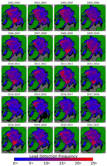
Figure 1.
Winter lead frequency by year, reported as the percentage of days between November and April with a lead detection at each location. Gray indicates locations where the sea ice mask [27] shows no continuous sea ice, and black indicates area where no leads are detected.

Figure 2.
Winter lead frequency by month, reported as the aggregate percentage of each month, November through April, from 2002 to 2022.
As cloud coverage can obscure leads at thermal infrared wavelengths, analysis of daily lead detections would be incomplete without analysis of changes in cloud coverage. Recent studies [29,30,31] have shown cloud coverage has been increasing over the Arctic. Our own analysis of the MODIS clear sky mask [32,33] over the winter seasons since 2002 in the Arctic is shown by year in Figure 3, by month in Figure 4, and quantitatively in Figure 5. Seasonally, comparing Figure 1 and Figure 3 regions of high lead detection frequency tend to correspond with regions with higher clear sky frequencies, and locations with relatively low lead detection frequency tend to have lower rates of clear sky coverage. Comparing monthly results in Figure 2 and Figure 4, clear sky frequency is generally lower in November and April, which also corresponds with months with low lead detection frequencies. Overall, we observe a decrease in clear sky observations over sea ice on the order of 3.5% per decade (Figure 5). December has a relatively small decrease in clear sky observations on the order of 2.9% per decade. Larger decreases of 5.1% and 5.6% per decade are observed in February and March. Similarly, it is important to consider how a decrease in the extent of sea ice could cause a reduction in the area in which lead formation is possible. The majority of the sea ice area is lost in the warm season while ice coverage in the Arctic remains high through the majority of the winter season as shown in Figure 6; quantitative results are shown in Figure 7. While there is some ice area loss, the amount of area lost is relatively small and limited to the marginal ice zone. Further, relatively few leads are detected in the marginal ice zone; the majority of the lead detections are in areas where there is sea ice all winter long. Some of this may be an artifact of a detection bias; leads are harder to detect in the marginal ice zones because of lower thermal contrast between leads and open water. Additionally, ice floes have a higher velocity than pack ice, and the lead detection technique is dependent on the assumption that leads move slow enough that they will persist at the same location over a span of multiple satellite overpasses. Due to these factors, our work focuses on leads within the ice pack, and within the ice pack we do not find a correlation between the rate of change of ice cover and the proportion of lead area to ice area.
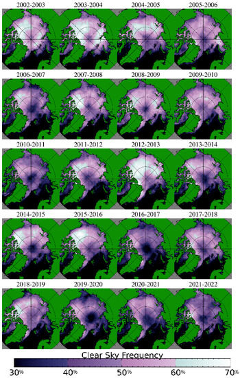
Figure 3.
Winter clear sky frequency by year, reported as the percentage of probably clear or confidently clear overpasses in the MODIS cloud mask [32,33] divided by the number of total overpasses from November to April. Only overpasses over continuous sea ice are considered.

Figure 4.
Winter clear sky frequency by month, reported as the percentage of probably clear or confidently clear overpasses in the MODIS cloud mask [32,33] divided by the number of total overpasses from November 2002 through April 2020. Only overpasses over continuous sea ice are considered.
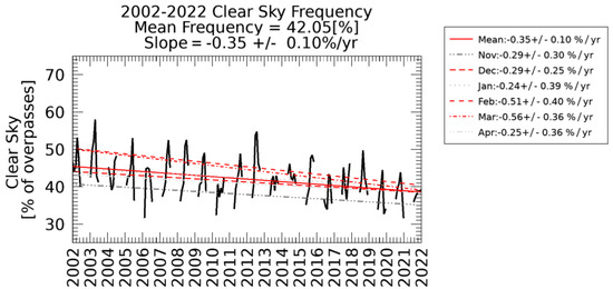
Figure 5.
Monthly clear sky frequency for winter months November 2002 through April 2022 as measured by the number of clear sky overpasses in the MODIS cloud mask [32,33] divided by total overpasses. Statistically significant decreases are in red, and shades of gray are used for months with no statistically significant trend.
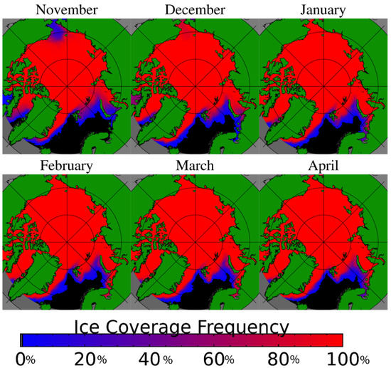
Figure 6.
Monthly ice coverage [27] for the winter months of November 2002 through April 2022.

Figure 7.
Sea ice extent [27] in terms of the percentage of ocean covered by sea ice for the winter months of November 2002 through April 2022, reported as a monthly average of the daily ice coverage. Statistically significant decreases are in red, and shades of gray are used for months with no statistically significant trend.
To interpret trends in lead detection, results are presented in a few different ways in Figure 8. Leads are shown as a percentage of the ocean area (Panel A), as a percentage of the sea ice area (Panel B), and as total area (Panel C). There is a slight decrease in lead area as a percentage of the ocean area (A) and cumulative lead area (C), but no statistically significant trend as a proportion of sea ice area (B). An interpretation of these results is that lead detection area is decreasing at about the same rate that sea ice is decreasing. This might be expected as lead detection frequency normalized by sea ice area is relatively constant while absolute lead detection area is decreasing. However, this may be a coincidence rather than causation. As previously discussed, there are relatively few lead detections in the marginal ice zone (where there are changes in ice coverage), so the change in lead area divided by ice area is largely driven by a change in the denominator rather than the numerator. On the other hand, a decrease in clear sky (increase in cloudiness) makes it difficult to attribute a change in lead detection frequency to a change in the formation of leads as opposed to a detection bias where there is a decrease in clear sky coverage that is making leads increasingly difficult to detect. Sky coverage appears to be the more important factor and may suggest that lead activity is increasing despite a decrease in detections. It is interesting to note that the local minima in lead activity occurs in November and April while there is variability year to year with the local maxima in lead activity occurring anytime between December and March. These trends do not follow the pattern in ice area (see Figure 7) but more closely follow the pattern in clear sky frequency (see Figure 5).
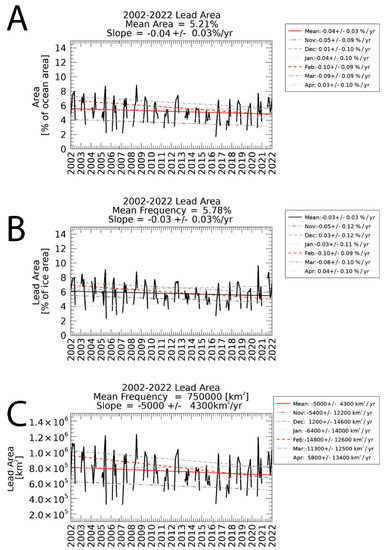
Figure 8.
Lead areas represented in three different ways. In Panel (A), lead area is given as the average daily percent of the ocean covered by leads. Panel (B) shows lead detection frequency as sea ice lead areas divided sea ice areas. In Panel (C), daily average area covered by leads is shown. Statistically significant decreases are in red, and shades of gray are used for months with no statistically significant trend.
Studies such as Qu et al. [9] have examined the relationship between cloud coverage and lead area. We have expanded that type of analysis to look at the relationship between clear sky frequency and lead detection frequency as illustrated in Figure 9. In Panel A, monthly lead detection frequency can be approximated over the range of clear sky frequency between 25–55% by Equation (1):
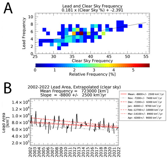
Figure 9.
The relationship between clear sky frequency and lead detection is shown in Panel (A), with a density plot of the monthly percentage of clear sky observations and the corresponding average monthly lead detection frequency for the winter months between November 2002 through April 2022. In Panel (B), the extrapolated lead area is shown over the same time period. Statistically significant decreases are in red, and shades of gray are used for months with no statistically significant trend.
With the equation for lead frequency, it is possible to extrapolate or calculate an expected lead detection frequency (in Panel B) as a function of clear sky frequency (Figure 3). This is not to suggest that there is a causal relationship between clear sky and lead, but rather a way to approximate the detection bias caused by the presence of clouds. This linear relationship is only valid on a monthly time scale and will fail when clear sky frequency is above 55% or below 25%. Lead detection may still be possible in the presence of clouds either because the cloud coverage may not persist all day long or the cloud may be optically thin enough that the warm lead may radiate through some clouds. Equation (1) will not be valid to estimate lead frequency on a daily basis where clear sky frequency can range from 0% or 100%. While it is possible to conduct an analysis of trends based on means from subsets of days and locations under ideal conditions (where clear sky conditions persist all day long), the subset is too small to be useful in a time series analysis. Furthermore, the relationship between the clear sky frequency and lead frequency is derived on monthly data, and is not intended to be used to derive the daily sea ice lead frequency and area. The linear model is only valid on a monthly basis, where clear sky frequencies tend to span the range of 25–55%. There are feedback relationships that would suggest that the heat and moisture fluxes associated with leads can contribute to cloud formation; the presence of clouds contributes to atmospheric warming [34] and this warming may also make the ice more prone to fracturing. Overall, our assumption is that lead formation is still largely caused by ice deformation and stress, and is largely independent of sky cover. However, there is a distinction between the formation of leads and lead detection. Our finding is that lead detection varies as a function of clear sky fraction. The extrapolated results show that there was a larger decrease in lead area: −8800 km2/year (Figure 9B), and that the loss was larger than was observed: −5000 km2/year (Figure 8B).
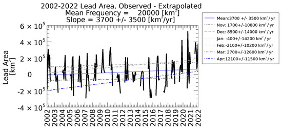
Since the decrease in lead detections extrapolated from clear sky frequency (from Figure 9, Panel B) exceeds the rate of decrease in observed lead area (Figure 8, Panel C), the conclusion is that leads may actually be increasing, but becoming increasingly difficult to detect because of the increasing cloud cover. In Figure 10, leads are shown to be increasing seasonally at a rate of 3700 +/− 3500 km2 per year. April has the largest and is the only statistically significant month, with an increase of 12,100 +/−11,500 km2 per year. The caveat is that the trends are small relative to the size of the domain and the uncertainty tends to be on the same order of magnitude as the slope. Other than the seasonal trend and April, no other months have statistically significant trends. This appears to be a result of intra-season variability, and there is an overall seasonal trend, but the month in which lead activity peaks can be any month between December to March and there is little correlation between years for what month the peak will occur. There are also some multi-year patterns to consider. From about 2004 through 2007, there was little trend, followed by an increasing trend from 2007 through 2010, then another decrease starting in 2010 through around 2016, and finally an increasing trend from 2016 through 2022. While the results are fit to a linear regression, given the cyclical nature of the results, it might not be appropriate to try to extrapolate lead trends into the future. The current upward trend may continue, or it remains possible that there will be more periods of flat or decreasing leads. Future work will have the benefit of more data points as the archive of years grows in future years. Additionally, analysis of trends on a regional or sub-seasonal basis similar to other studies [9,18] could be beneficial.
One of the primary advantages of our new lead detection technique [14] is its portability between satellites, resulting in a similar detection performance between MODIS [25] and VIIRS [26]. Aggregate detection results from the winter of 2017–2018 (the first season after NOAA-20 became operational) through 2021–2022 are shown in Figure 11. Of the MODIS lead detections, 28% are unique to MODIS (72% are also detecting by VIIRS). Additionally, of the VIIRS lead detections, 27% are unique to VIIRS (73% are also detected by MODIS). Approximately 57% of leads are detected by both MODIS and VIIRS, 22% are unique to MODIS, and 21% are unique to VIIRS. Further, the majority of the leads that are detected by both satellites tend to be within the continuous sea ice. In contrast, leads that are detected by one satellite tend to be along the ice edge. MODIS tends to detect more unique leads along the Greenland–Iceland–Norwegian (GIN) Seas, Barents Sea, Kara Sea, and Laptev Sea. VIIRS tends to detect more unique leads in the Chukchi Sea, Beaufort Sea, Canada Basin, and Baffin Bay areas. Future work will examine the characteristics of lead detections by MODIS and VIIRS, with the assumption that VIIRS, with finer spatial resolution (375 m), would be able to detect narrower leads than the 1 km resolution MODIS. Outside of the marginal ice zone, the initial analysis suggests there is minimal detection bias between MODIS and VIIRS. Particularly in the marginal ice zone, differences in coverage patterns (fewer overpasses at lower latitudes) and faster moving leads along the ice edge may be the primary reasons for the product differences. The MODIS mission is nearing its end-of-life and the VIIRS mission will soon be extending to JPSS-2 (the future NOAA-21), so it will become increasingly important to examine cross-platform continuity in order to develop a leads climatology that extends past the duration of the MODIS mission.
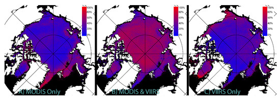
Figure 11.
Lead detections from November 2017 through April 2022. Panel (A) shows the percentage of lead detections that are unique to MODIS, Panel (B) shows the percentage of lead detections that are co-located between MODIS and VIIRS, and Panel (C) shows the percentage of lead detections that are unique to VIIRS.
4. Discussion
The AI-based product [25,26] is a replacement for the earlier or legacy product [15], developed by the same principal group of researchers. The primary difference is that AI replaced more traditional image processing techniques. The differences in the product are illustrated in Figure 12. The AI technique [25] has higher detection rates nearly everywhere with the exception of the marginal ice zones. Moreover, note that the product comparison is calculated where both products provide coverage; the legacy product was limited to clear sky conditions and had a scan angle limitation that prevented coverage near the North Pole. Lead detections outside of the ice pack are excluded by an ice mask [27]. The AI technique shows fewer detections in the marginal ice zones, though not necessarily less skill because this region is prone to false detections in the legacy product. Outside of the marginal ice zone, the AI technique consistently detects more leads. The current detection model was trained primarily to detect leads within the ice pack, but a future detection model could be trained specifically for application in the marginal ice zone. Similarly, this AI model was designed for detection across the whole Arctic. It would be possible to train future models to optimize detections in specific geographic regions.

Figure 12.
Comparison of the relative detection frequency between the AI-based lead detection [25] and legacy [12] and products. Lead products from November through April 2002–2022. Yellows and reds are used where the AI detection rate is higher, blue where legacy is higher, green indicates regions with identical detection rates, and black is outside of the ice pack.
Willmes and Heinemann have a published dataset [24] of leads from January to April of 2003 through 2015. A comparison with the AI product [25] over the same time period is shown in Figure 13. Our new technique, again, has a slightly higher detection rate almost everywhere inside the pack ice, whereas the Willmes and Heinemann technique has a higher detection rate in the marginal ice zones. This is further evidence that the AI product [25] does well at detecting leads within the continuous sea ice pack, but detection performance decreases in the marginal ice zone where it becomes more difficult to differentiate between leads and ice floes, as the leads become wider and faster moving.

Figure 13.
Comparison of the relative detection frequency between the Hoffman [13] and Willmes [21] lead products from 2003–2015. Yellows and reds are used where the Hoffman detection rate is higher, blue to black where Willmes is higher, and green indicates regions with identical detection rates.
Reiser et al. [14] is a follow up to the earlier Willmes and Heinemann technique, and lead detection results have been published in a dataset [35] from 2002 through 2019. The Reiser et al. results are reported as lead frequency generalized over the entire time series; daily products from individual days have not been published. This makes direct comparisons more difficult. Two comparisons are presented in Figure 14. If the aggregate of daily Hoffman et al.’s AI results [25] are compared directly against that of Reiser et al.’s results, the AI technique has a lower detection rate almost everywhere, shown in Figure 14, Panel A. However, Reiser et al.’s dataset is described as an estimate of daily lead frequency that accounts for cloud coverage. So, if Hoffman et al.’s results [25] are limited to the subset of locations that have probably clear or confidently clear sky in the MODIS sky cover product [32,33], then the Hoffman technique has a higher detection rate inside the continuous sea ice and lower detection rates around the marginal ice zones. Panel B in Figure 14 is more applicable in terms of a direct comparison. The primary disadvantage of Reiser et al.’s dataset is that by only reporting an average of leads, it makes an implicit assumption that leads are not changing with time.
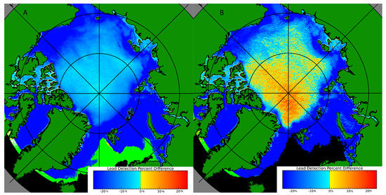
Figure 14.
Comparison of the relative detection frequency between the Hoffman [25] and Reiser [35] lead products from 2002–2019. Yellows and reds are used where the Hoffman detection rate is higher, blue to black where Reiser et al.’s is higher; green indicates regions with identical detection rates. The detection rate is the number of days with lead divided by the number of days with product coverage. In Panel (A), the detection rate for all sky cover is shown. In Panel (B), the detection rate is given from the subset of locations and days where the MODIS clear sky is probably clear in all of the daily overpasses.
5. Conclusions
The AI lead detection results are an improvement over earlier lead detection products. The advantages of the AI-based lead detection product is that it is trainable and adaptable to new instruments, which allows for climate-scale studies of leads to continue after the end of the MODIS mission using current and future VIIRS instruments. With an extensive time series of the sea ice lead products now available for the Arctic Ocean, the initial analysis shows a small but statistically significant seasonal decline in detected lead areas. Meanwhile, there is also a decrease in the amount of clear sky coverage. The key finding is that the decline in lead detection area is smaller than would be expected based on extrapolation of the relationship between lead detection frequency and clear sky frequency. Due to inter-season and intra-season variability, a non-linear representation of the slope may be more appropriate to approximate the long-term trend. Due to the non-linearity of the seasonality of the trends, the magnitude of linear regression results in a small trend that is on the same order of magnitude as the range of uncertainty. However, the conclusion is that leads are not becoming less likely to occur, but less likely to detect. After the effects of cloud cover is removed, leads are likely increasing at a rate of 3700 +/− 3500 km2 per year. Although the trends are small, they are nonetheless important in the context of a thinning Arctic Ocean sea ice cover.
Future work will examine lead characteristics (width, length, orientation) and causes of leads (wind stress, ice deformation). For example, if leads are becoming smaller or thinner, that could help explain why leads becoming harder to detect, and that could be independent of changes in cloud coverage. More rigorous work can be conducted to better approximate the relationship between clouds and leads; comparing results from microwave-based product could help quantify how often clouds obscure leads from detection as well as how often the presence of leads may contribute to the formation of clouds. Additionally, detection performance in the marginal ice zone was not prioritized when training the model; a new detection model could be trained specifically to focus on the areas that are known weaknesses of the current detection model. An alternate approach would be to extrapolate lead occurrences under cloudy or partly cloudy conditions. Ultimately, the intent here is to present a comparison of lead detection results over a twenty-year time period. The users’ application may dictate if the dataset should be used natively (as daily lead detections), combined to produce aggregate results over a time series, and/or extrapolated with the aim to minimize the detection bias caused by cloud coverage. The best representation of daily lead activity would likely be achieved from a composite of multiple sensor types. Moderate resolution infrared imagers such as MODIS and VIIRS offer wide spatial coverage, but these products could be supplemented with a cloud penetrating microwave-based product and/or an altimeter-based product.
Author Contributions
Methodology, J.P.H. and Y.L.; software, J.P.H. and Y.L.; validation, J.P.H.; formal analysis, J.P.H.; investigation, J.P.H.; resources, J.P.H., Y.L., and J.R.K.; data curation, J.P.H. and Y.L.; writing—original draft preparation, J.P.H.; writing—review and editing, J.P.H., S.A.A., Y.L., and J.R.K.; visualization, J.P.H.; supervision, S.A.A.; project administration, S.A.A.; funding acquisition, S.A.A. All authors have read and agreed to the published version of the manuscript.
Funding
This research was funded by NASA, grant number 80NSSC18K0786.
Data Availability Statement
The U-Net model files, example code, validation masks, and product results used in this paper are available via anonymous ftp at ftp://frostbite.ssec.wisc.edu/unet (accessed 1 July 2022). U-Net leads datasets are available on DRYAD, MODIS at https://doi.org/10.5061/dryad.79cnp5hz2, and VIIRS at https://doi.org/10.5061/dryad.1vhhmgqwd.
Acknowledgments
The Aqua and Terra MODIS, and SNPP and NOAA-20 VIIRS datasets were acquired from the Level-1 and Atmosphere Archive & Distribution System (LAADS) Distributed Active Archive Center (DAAC), located in the Goddard Space Flight Center in Greenbelt, Maryland (https://ladsweb.nascom.nasa.gov/ (accessed 1 July 2022)) and the Atmosphere SIPS located at the University of Wisconsin–Madison (https://sips.ssec.wisc.edu (accessed 1 July 2022)). The Willmes and Heinemann leads dataset was acquired from PANGAEA (https://doi.pangaea.de/10.1594/PANGAEA.854411 (accessed 1 July 2022). The Reiser et al. leads dataset was acquired from PANGAEA (https://doi.pangaea.de/10.1594/PANGAEA.917588 (accessed 1 July 2022)). The views, opinions, and findings contained in this report are those of the author(s) and should not be construed as an official National Oceanic and Atmospheric Administration or US Government position, policy, or decision.
Conflicts of Interest
The authors declare no conflict of interest.
References
- Global Cryosphere Watch Glossary. Available online: https://globalcryospherewatch.org/reference/glossary.php (accessed on 5 October 2022).
- Andreas, E.L.; Persson, P.O.G.; Grachev, A.A.; Jordan, R.E.; Horst, T.W.; Guest, P.S.; Fairall, C.W. Parameterizing Turbulent Exchange over Sea Ice in Winter. J. Hydrometeorol. 2010, 11, 87–104. (In English) [Google Scholar] [CrossRef]
- Miles, M.W.; Barry, R.G. A 5-year satellite climatology of winter sea ice leads in the western Arctic. J. Geophys. Res. Ocean. 1998, 103, 21723–21734. [Google Scholar] [CrossRef]
- Maykut, G.A. Energy exchange over young sea ice in the central Arctic. J. Geophys. Res. Ocean. 1978, 83, 3646–3658. [Google Scholar]
- Lüpkes, C.; Vihma, T.; Birnbaum, G.; Wacker, U. Influence of leads in sea ice on the temperature of the atmospheric boundary layer during polar night. Geophys. Res. Lett. 2008, 35, 3. [Google Scholar] [CrossRef]
- Liu, Y.; Key, J.R.; Liu, Z.; Wang, X.; Vavrus, S.J. A cloudier Arctic expected with diminishing sea ice. Geophys. Res. Lett. 2012, 39, 5. [Google Scholar] [CrossRef]
- Myers, D.C.; Lawler, M.J.; Mauldin, R.L.; Sjostedt, S.; Dubey, M.; Abbatt, J.; Smith, J.N. Indirect Measurements of the Composition of Ultrafine Particles in the Arctic Late-Winter. J. Geophys. Res. Atmos. 2021, 126, e2021JD035428. [Google Scholar] [CrossRef]
- Wang, Q.; Ilicak, M.; Gerdes, R.; Drange, H.; Aksenov, Y.; Bailey, D.A.; Bentsen, M.; Biastoch, A.; Bozec, A.; Böning, C.; et al. An assessment of the Arctic Ocean in a suite of interannual CORE-II simulations. Part I: Sea ice and solid freshwater. Ocean. Model. 2016, 99, 110–132. [Google Scholar] [CrossRef]
- Qu, M.; Pang, X.; Zhao, X.; Lei, R.; Ji, Q.; Liu, Y.; Chen, Y. Spring leads in the Beaufort Sea and its interannual trend using Terra/MODIS thermal imagery. Remote Sens. Environ. 2021, 256, 112342. [Google Scholar] [CrossRef]
- Petty, A.A.; Bagnardi, M.; Kurtz, N.T.; Tilling, R.; Fons, S.; Armitage, T.; Horvat, C.; Kwok, R. Assessment of ICESat-2 Sea Ice Surface Classification with Sentinel-2 Imagery: Implications for Freeboard and New Estimates of Lead and Floe Geometry. Earth Space Sci. 2021, 8, e2020EA001491. [Google Scholar] [CrossRef]
- Nguyen, A.T.; Heimbach, P.; Garg, V.V.; Oca?a, V.; Lee, C.; Rainville, L. mpact of Synthetic Arctic Argo-Type Floats in a Coupled Ocean?Sea Ice State Estimation Framework. J. Atmos. Ocean. Technol. 2020, 37, 1477–1495. (In English) [Google Scholar] [CrossRef]
- Lewis, B.J.; Hutchings, J.K. Leads and Associated Sea Ice Drift in the Beaufort Sea in Winter. J. Geophys. Res. Ocean. 2019, 124, 3411–3427. [Google Scholar] [CrossRef]
- Willmes, S.; Heinemann, G. Sea-ice wintertime lead frequencies and regional characteristics in the Arctic, 2003–2015. Remote Sens. 2015, 8, 4. [Google Scholar]
- Reiser, F.; Willmes, S.; Heinemann, G. A New Algorithm for Daily Sea Ice Lead Identification in the Arctic and Antarctic Winter from Thermal-Infrared Satellite Imagery. Remote Sens. 2020, 12, 1957. [Google Scholar]
- Hoffman, J.P.; Ackerman, S.A.; Liu, Y.; Key, J.R. The Detection and Characterization of Arctic Sea Ice Leads with Satellite Imagers. Remote Sens. 2019, 11, 521. [Google Scholar] [CrossRef]
- Hoffman, J.P.; Ackerman, S.A.; Liu, Y.; Key, J.R.; McConnell, I.L. Application of a Convolutional Neural Network for the Detection of Sea Ice Leads. Remote Sens. 2021, 13, 4571. [Google Scholar]
- Röhrs, J.; Kaleschke, L. An algorithm to detect sea ice leads by using AMSR-E passive microwave imagery. Cryosphere 2012, 6, 343–352. [Google Scholar]
- Li, M.; Liu, J.; Qu, M.; Zhang, Z.; Liang, X. An Analysis of Arctic Sea Ice Leads Retrieved from AMSR-E/AMSR2. Remote Sens. 2022, 14, 969. [Google Scholar]
- Zhang, X.; Zhu, Y.; Zhang, J.; Wang, Q.; Shi, L.; Meng, J.; Fan, C.; Liu, M.; Liu, G.; Bao, M. Assessment of Arctic Sea Ice Classification Ability of Chinese HY-2B Dual-Band Radar Altimeter During Winter to Early Spring Conditions. IEEE J. Sel. Top. Appl. Earth Obs. Remote Sens. 2021, 14, 9855–9872. [Google Scholar] [CrossRef]
- Liang, Z.; Pang, X.; Ji, Q.; Zhao, X.; Li, G.; Chen, Y. An Entropy-Weighted Network for Polar Sea Ice Open Lead Detection From Sentinel-1 SAR Images. IEEE Trans. Geosci. Remote Sens. 2022, 60, 1–14. [Google Scholar] [CrossRef]
- Galbiati, F.; McConnell, I.L.; Hoffman, J.P.; Greenwald, T. Sea-Ice Leads Detection in Enhanced AMSR-E Data through a Convolutional Neural Network. Unpublished manuscript. 5 October 2022. [Google Scholar]
- Asadi, N.; Scott, K.A.; Komarov, A.S.; Buehner, M.; Clausi, D.A. Evaluation of a Neural Network With Uncertainty for Detection of Ice and Water in SAR Imagery. IEEE Trans. Geosci. Remote Sens. 2020, 59, 247–259. [Google Scholar] [CrossRef]
- Han, Y.; Liu, Y.; Hong, Z.; Zhang, Y.; Yang, S.; Wang, J. Sea Ice Image Classification Based on Heterogeneous Data Fusion and Deep Learning. Remote Sens. 2021, 13, 592. [Google Scholar] [CrossRef]
- Khaleghian, S.; Ullah, H.; Krmer, T.; Eltoft, T.; Marinoni, A. Deep Semi-Supervised Teacher-Student Model based on Label Propagation for Sea Ice Classification. IEEE J. Sel. Top. Appl. Earth Obs. Remote Sens. 2021, 14, 10761–10772. [Google Scholar] [CrossRef]
- Hoffman, J. MODIS sea ice leads detections using a U-Net, 25 July 2022; Distributed by Dryad. [CrossRef]
- Hoffman, J. VIIRS sea ice leads detections using a U-Net, 2 September 2022; Distributed by Dryad. [CrossRef]
- Meier, W.; Fetterer, F.; Windnagel, A.; Stewart, S. NOAA/NSIDC Climate Data Record of Passive Microwave Sea Ice Concentration, Version 4. Distributed by National Snow and ice Data Center. 2021. [Google Scholar] [CrossRef]
- Brodzik, M.J. EASE-Grid: A Versatile Set of Equal-Area Projections and Grids. In Discrete Global, Grids; Goodchild, M., Knowles, K.W., Eds.; National Center for Geographic Information & Analysis: Santa Barbara, CA, USA, 2002. [Google Scholar]
- Wang, X.; Liu, J.; Yang, B.; Bao, Y.; Petropoulos, G.P.; Liu, H.; Hu, B. Seasonal Trends in Clouds and Radiation over the Arctic Seas from Satellite Observations during 1982 to 2019. Remote Sens. 2021, 13, 3201. [Google Scholar]
- Jun, S.-Y.; Ho, C.-H.; Jeong, J.-H.; Choi, Y.-S.; Kim, B.-M. Recent changes in winter Arctic clouds and their relationships with sea ice and atmospheric conditions. Tellus A Dyn. Meteorol. Ocean. 2016, 68, 29130. [Google Scholar] [CrossRef]
- Liu, Y.; Key, J.R.; Wang, X. The Influence of Changes in Cloud Cover on Recent Surface Temperature Trends in the Arctic. J. Clim. 2008, 21, 705–715. [Google Scholar] [CrossRef]
- Ackerman, S. MODIS Atmosphere L2 Cloud Mask Product. NASA MODIS Adaptive Processing System; Goddard Space Flight Center: Greenbelt, MD, USA, 2015. [Google Scholar] [CrossRef]
- Ackerman, S. 2015 MODIS Atmosphere L2 Cloud Mask Product. NASA MODIS Adaptive Processing System; Goddard Space Flight Center: Greenbelt, MD, USA. [CrossRef]
- Liu, Y.; Key, J.R. Assessment of Arctic Cloud Cover Anomalies in Atmospheric Reanalysis Products Using Satellite Data. J. Clim. 2016, 29, 6065–6083. (In English) [Google Scholar] [CrossRef]
- Reiser, F.; Willmes, S.; Heinemann, G. Daily sea ice lead data for Arctic and Antarctic; PANGAEA Dara Publisher for Earth and Environmental Science: Bremen, Germany, 2020. [Google Scholar] [CrossRef]


Publisher’s Note: MDPI stays neutral with regard to jurisdictional claims in published maps and institutional affiliations. |
© 2022 by the authors. Licensee MDPI, Basel, Switzerland. This article is an open access article distributed under the terms and conditions of the Creative Commons Attribution (CC BY) license (https://creativecommons.org/licenses/by/4.0/).