Mapping Arctic Sea-Ice Surface Roughness with Multi-Angle Imaging SpectroRadiometer

Abstract

Sea-ice surface roughness (SIR) is a crucial parameter in climate and oceanographic studies, constraining momentum transfer between the atmosphere and ocean, providing preconditioning for summer-melt pond extent, and being related to ice age and thickness. High-resolution roughness estimates from airborne laser measurements are limited in spatial and temporal coverage while pan-Arctic satellite roughness does not extend over multi-decadal timescales. Launched on the Terra satellite in 1999, the NASA Multi-angle Imaging SpectroRadiometer (MISR) instrument acquires optical imagery from nine near-simultaneous camera view zenith angles. Extending on previous work to model surface roughness from specular anisotropy, a training dataset of cloud-free angular reflectance signatures and surface roughness, defined as the standard deviation of the within-pixel lidar elevations, from near-coincident operation IceBridge (OIB) airborne laser data is generated and is modelled using support vector regression (SVR) with a radial basis function (RBF) kernel selected. Blocked k-fold cross-validation is implemented to tune hyperparameters using grid optimisation and to assess model performance, with an $R^2$ (coefficient of determination) of 0.43 and MAE (mean absolute error) of 0.041 m. Product performance is assessed through independent validation by comparison with unseen similarly generated surface-roughness characterisations from pre-IceBridge missions (Pearson’s r averaged over six scenes, r = 0.58, p < 0.005), and with AWI CS2-SMOS sea-ice thickness (Spearman’s rank, $r^s$ = 0.66, p < 0.001), a known roughness proxy. We present a derived sea-ice roughness product at 1.1 km resolution (2000–2020) over the seasonal period of OIB operation and a corresponding time-series analysis. Both our instantaneous swaths and pan-Arctic monthly mosaics show considerable potential in detecting surface-ice characteristics such as deformed rough ice, thin refrozen leads, and polynyas.

1. Introduction

Sea-ice surface roughness (SIR) is a crucial parameter for climate studies, in addition to more localized navigational applications. Numerous characterisations of surface roughness exist, principally falling into three categories of descriptors: statistical height, extreme value height, and textural [1]. In this study, we focus on roughness characterisations based on the second central moment of elevation probability density functions; consequently, SIR is defined here as the standard deviation of elevation measurements within a specified footprint (to a best-fit plane). The roughness of sea ice spans multi-magnitudinal length scales from microscopic to vertical ridge structures of several metres. In this work, we focus on the larger end (0.1–10 m) of this spectrum corresponding to the topography resolved by airborne lidar instruments.

Surface roughness can be used as a proxy for ice age and thickness, as the surface morphology of multi-year ice is deformed by convergence and divergence, creating pressure ridges, keels, leads, and sastrugi from wind interactions [2]. Sea-ice roughness is critical for coastal communities [3] and has commercial implications on the future potential navigability of the Arctic Ocean [4]. Evolution within the context of rapid climate change remains uncertain, with future ice predicted to be younger and thinner but also more dynamic and likely to deform and ridge more in certain regions [5]. As roughness places constraints on drag coefficients [6], it forms a crucial component of modelling momentum transfer between the atmosphere and ocean [7]. Sea-ice surface morphology also provides preconditioning for summer-melt pond formation [8] and, thus, September minimum extent via ice-albedo feedback [9]. Large-scale sea-ice roughness has been acknowledged as a potential source of bias for remote-sensing techniques such as radar altimetry retracking [10]. Yet, high-resolution, multi-decadal, pan-Arctic characterizations of sea-ice surface roughness remain evasive.

Scatterometers such as QuikSCAT and SMOS have been used extensively to characterise properties of sea ice such as permittivity [11] and ice class (discrimination between first-year and multi-year ice) [12] from backscatter coefficients, and have been shown to capture surface-roughness characteristics [13]. SAR imagery has extensively been used to characterize ice type, including for maritime purposes [14,15], and its use has demonstrated quantitative skill for the inference of ice thickness [16] and extraction of roughness-related features such as pressure ridges and rubble fields [17]. More recently, C-band SAR imagery has been utilised for surface-roughness retrieval at the snow–ice interface [18]. Radar altimetry can indirectly inform on the roughness within the footprints intercepted by the beams, as radar echoes are sensitive to the roughness within the footprint of the instrument, with larger leading-edge widths of the radar echoes an indication of rougher surfaces [10]. Laser altimeters yield a direct estimate of the elevation changes at the resolution of the instrument. ICESat-2 has been demonstrated to successfully produce measurements of surface roughness on a pan-Arctic scale [19]; however, it should be noted that this does not extend to a multi-decadal timescale.

The Airborne Topographic Mapper (ATM) is a laser altimeter which forms part of the suite of instruments onboard NASA Operation IceBridge (2009–2019). Surface-elevation measurements are obtained in a conical spiral with a vertical precision of 3 cm and a swath width of approximately 250 m, variable with survey altitude. IceBridge and other similar airborne campaigns (e.g., EM-Bird) are constrained to individual campaigns predominantly around Greenland, the Beaufort Sea, and the Canadian islands and, thus, are limited in spatial extent and are biased to the Arctic spring.

Multi-angle Imaging SpectroRadiometry (MISR) has been proposed as another promising technique to characterize sea-ice surfaces and relies on the fact that rougher ice surfaces are optically backward scattering relative to their smoother counterparts. As such, the relative proportion of optical backscatter to forescatter can be used to reveal surface characteristics of sea ice. MISR was launched into a geocentric low-Earth sun-synchronous orbit as part of Terra-1 in December 1999. Radiance spectra are recorded with an array of nine cameras oriented at regularly spaced angles (±70.5°, ±60.0°, ±45.6°, ±26.1°, ±0°) over a reconnaissance interval of seven minutes, and over three visible light wavelengths (Blue, 446 nm; Green, 558 nm; Red, 672 nm; NIR band, 867 nm) using a push broom scanner with a CCD (charge-coupled device) array, as illustrated in Figure 1.

Pixel sampling occurs at either 275 m or 1.1 km, depending on the camera, band, and operational mode. For bandwidth conservation purposes, only the red band and the An (0°; nadir) camera have 275 m resolution for all bands (

Table 1. MISR multi-angle imaging characteristics to illustrate the different view angles and resolutions for the nine MISR cameras and four bands, assuming primary operation in global mode.

Camera	View Angle	Resolution (km)
		Blue	Green	Red	NIR
Df	+70.5°	1.1	1.1	0.275	1.1
Cf	+60.0°	1.1	1.1	0.275	1.1
Bf	+45.6°	1.1	1.1	0.275	1.1
Af	+26.1°	1.1	1.1	0.275	1.1
An	0.0°	0.275	0.275	0.275	0.275
Aa	−26.1°	1.1	1.1	0.275	1.1
Ba	−45.6°	1.1	1.1	0.275	1.1
Ca	−60.0°	1.1	1.1	0.275	1.1
Da	−70.5°	1.1	1.1	0.275	1.1

); activation of the local mode for 275 m resolution fore and aft cameras in the non-red band is by request only and the spatial and temporal catalogues for these data products is poor relative to the global mode products. Terra-1 orbits at an altitude of 705 km and with an inclination of 98.3° in ascending (northwards) and descending (southwards) passes, such that the extreme extent of polar coordinates (north of ≈84°) are not covered. The temporal catalogue spans from March 2000 to present, on a repeat of 16 days with a cycle of 233 unique paths, which are each split into 180 blocks. The re-imaging interval varies according to latitude, with more frequent resampling intervals over polar regions (around three days) compared to the equatorial regions (up to nine days). The use of angular-reflectance signatures from the MISR instrument as proxies for surface roughness has been applied to land ice [20,21] by the use of the NDAI (normalised difference angular index), with this illustration of relative backscatter acting as a proxy for surface roughness.

$$NDAI=\frac{Ca-Cf}{Ca+Cf}$$

(1)

Ref. [22] proposes a 4D model of surface roughness derived from three components of MISR angular-reflectance signatures (An, Ca, and Cf; red) and coincident root mean square fitted elevation observations to a plane (from IceBridge ATM L2 Icessn Elevation, Slope, and Roughness [23]). The model uses a modified radius neighbours regression with a defined sphere of influence of 0.025. During prediction, training incidents within the sphere of influence of the queried components of the angular reflection signature are aggregated using a weighted mean of the number of within-pixel IceBridge platelets. This approach showed some skill in capturing roughness along individual airborne tracks validation in the form of reserved (not used for model construction) IceBridge tracks with an $R^2$ (coefficient of determination) of 0.52 for an IceBridge track over smooth sea ice, and 0.39 over a track containing rougher ice. This model relies exclusively on spectral features and does not contain any contextual information, such as relative azimuth or solar zenith. Moreover, only a limited subset of the available IceBridge campaigns is used to construct the 4-D model. Finally, whilst the model has been validated on a track-by-track basis, pan-Arctic applications are potentially uncertain due to the spatial biases intrinsic to the IceBridge reconnaissance, in that validation in the Russian sector is not possible using solely IceBridge tracks.

The utilisation of the near-instantaneous multiple-view-angle sampling of surface anisotropy from the MISR satellite has shown considerable promise in revealing surface morphologies, including surface roughness in the cryosphere. In this study, we extend this to multi-decadal pan-Arctic characterisations of sea-ice surface roughness through the non-linear regression modelling of angular reflectance signatures to laser altimeter measurements of surface roughness. Section two provides an overview of both the pre-processing applied to retrieve georeferenced and cloud-free angular-reflectance signature components and describes our processing chain for the retrieval of sea-ice surface roughness from MISR. In the following section, we present an overview of our derived roughness products, and a regional analysis. This is then followed by a section on product validation through comparison with independent roughness tracks and also with AWI CS2-SMOS ice thickness (Alfred Wegener Institute CryoSat-2-Soil Moisture and Ocean Salinity Merged Sea Ice Thickness [24]), a known roughness proxy.

2. Data and Methods

2.1. Data Products

The data products and versions outlined in

Table 2. A summary of the data fields, products, and versions used in this study and their respective purpose.

Data Field	Product (Version)	Short Name	Use
Latitude, Longitude, Elevation	IceBridge ATM L1B Qfit Elevation and Return Strength (V001) [25] IceBridge ATM L1B Elevation and Return Strength (V002) [26]	ILATM1B	To provide observations of surface roughness for the construction of training data
Cf *, Af *, An *, Aa *, Ca *	MISR Level 1B2 Ellipsoid Data (V003) [27]	MI1B2E	To provide observations of specular anisotropy used for model construction and application for conversion to roughness
View Azimuth, Solar Azimuth, Solar Zenith	MISR Geometric Parameters V002 [28]	MI1B2GEOP	To provide contextual solar and view geometries for modelling
SDCM	MISR Level 2 TOA/Cloud Classifier parameters (V003) [29]	MIL2TCCL	Cloud masking
ASCM	MISR Level 2 TOA/Cloud Height and Motion parameters (V001) [30]	MIL2TCSP	Cloud masking
Sea Ice By Ref, Ice Surface Temperature	MODIS/Terra Sea Ice Extent 5-Min L2 Swath 1km (Version 6) [31]	MOD29	Cloud masking and modelling
Latitude, Longitude	MODIS Level 1B Geolocation (Version 6) [32]	MOD03	Cloud masking
b19, b5, b13, b16	MODIS Level 1B Calibrated Radiances (Version 6) [33]	MOD021KM	Cloud shadow masking
U, V, X, Y	Polar Pathfinder Daily 25 km EASE-Grid Sea Ice Motion Vectors (Version 4) [34]	NSIDC-0116	Filtering
Latitude, Longitude, Analysis sea ice thickness	CryoSat-SMOS Merged Sea Ice Thickness (v202) [24]	AWI CS2-SMOS	Validation
Latitude, Longitude, Elevation	Pre-IceBridge ATM L1B Qfit Elevation and Return Strength, (V001) [35]	BLATM1B	Validation

* Red, NIR, and Green bands.

were implemented for various described purposes in this work. For each specific product, this table details the data layers used and defines conventional shorthand notation as well as providing a brief overview of how each data layer was used. More detailed explanations of the precise processing applied is outlined in the following sections below.

Ellipsoid-projected top-of-atmosphere (TOA) radiances for all the five view angles (from MI1B2E), as described in Table 2, were georeferenced and subset to the Arctic region (blocks 1–45). The MISR Toolkit [36] was employed for georeferencing and block stitching. Additional layers X and Y were created to describe a geolocation consistent with the Lambert azimuthal equal area projection associated with the EASE-2 grid (EPSG:6931). These radiances were then calibrated to TOA BRFs using standardised weighted radiance calibration via pre-computed factors within the same product and low-quality retrievals were removed (denoted by an RDQI ≤ 2). Imagery for the red channel and nadir viewing angle were down-scaled from 275 m resolution to 1.1 km by local mean averaging over a 4 × 4 block. From the geometric product (MI1B2GEOP), the azimuth and zenith of the solar and each viewing angles were extracted to define the orbital geometry, and the relative azimuth angle for each viewing camera calculated. As the magnitude of the atmospheric correction is small compared to the reflection from sea ice, and aerosol profiles over the study period are poorly resolved, atmospheric correction was not applied.

2.2. Cloud Masking

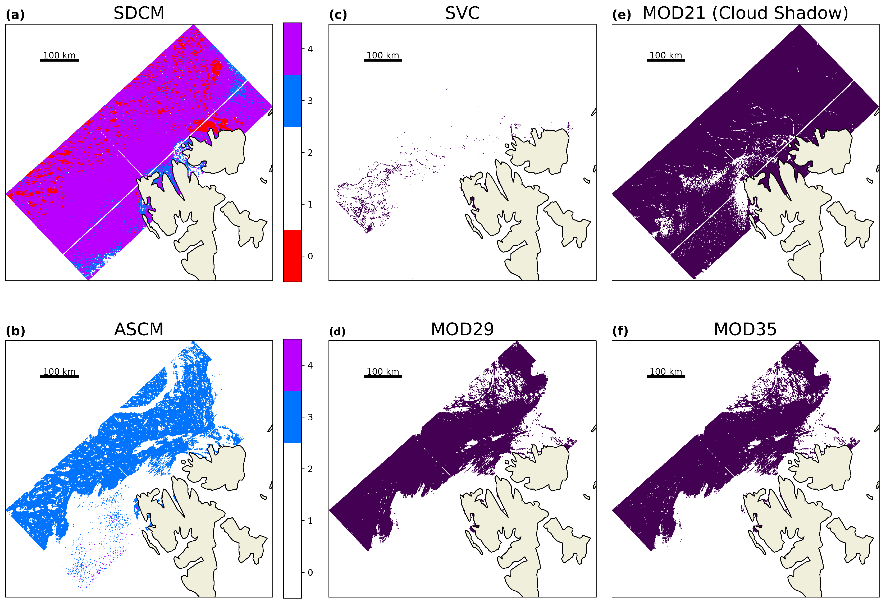
Cloud masking of scenes that include sea ice with high accuracy and coverage remains a substantial open problem for imagery from almost all EO satellites including the MISR satellite. Production-level cloud masks from this mission which are applicable to the cryosphere are of two natures, the Stereoscopically Derived Cloud Mask (SDCM) and the Angular Signature Cloud Mask (ASCM). The SVM scene classifier is currently at provisional-quality designation and was used for purposes of comparative illustration only.

The SDCM (Figure 2a) identifies clouds using an algorithm to measure parallax via camera-to-camera image matching from a combination of viewing angles [37], implemented to retrieve the altitude of the radiance reflecting layer, as such, pixels are denoted as either having originated from the surface of the ellipsoid (cloud-free), or from a higher altitude (both at high and low confidence). The limitations of this method mean that clouds are only retrieved at an altitude greater than 560 m [38], since below this corresponds to sub-pixel resolution, and only clouds with a high-enough optical thickness to have persistent features for a stereo-matching algorithm are detected. Two SDCM products are currently operational, based on differing stereo-matching algorithms for retrieval of stereo vectors [39]. In this project, we refer to the more recent SDCM contained in MIL2TCCL (TC_CLOUD), except where explicitly referenced. Comparisons with CERES determined that optimal performance of the SDCM occurs when no retrieval is treated as clear [40].

The ASCM (Figure 2b) implements a band-differenced angular signature (BDAS) between the blue and red bands (over sea ice) as a function of viewing angle, with a comparison against threshold values to determine cloud classification. As such, pixels are denoted as either cloud or not cloud (both at high and low confidence). This mask performs well with high-altitude clouds, since the relative contribution of Rayleigh scattering exhibits a large differential between these two bands, and decreases with the lower path radiance associated with higher clouds. By comparison with expertly labelled scenes in the Arctic, the performance of the ASCM is assessed at 76% accuracy with 80% coverage [42].

Another of the suite of instruments on board the Terra-1 platform is the MODIS (Terra) satellite. The MODIS satellite contains more spectral bands than the MISR sensor (36 compared to four) over a larger swath width of 2330 km, but only with a single nadir scan angle. As MISR and MODIS (TERRA) are both onboard the same instrument platform, there is near-simultaneous acquisition between these two sensors, and so MODIS (Terra) cloud masks are valid for MISR scenes and vice versa, subject to swath width constraints. The MOD35 cloud mask (Figure 2f) contains 48 bits to allow the mask to be configured for a variety of end-use purposes; the displayed mask is high-confidence clear pixels where thin cirrus cloud has not been detected. From MOD35-CALIPSO hit rates, MOD35 has been demonstrated to have an accuracy in excess of 90% for the region of interest [43]. Additionally shown is MOD29 (Figure 2d), a sea-ice surface temperature and extent product. In MOD29, pixels determined ‘certain-cloud’ by MOD35 are removed, and presence of sea ice is determined using a combination of NDSI, band thresholding, and a land mask from MOD03 (a geolocation product).

Visual inspection of multiple scenes demonstrated that MOD29 and the aforementioned implementation of MOD35 are broadly consistent, except in darker conditions, as the NDSI is only determined under good light conditions. Both MODIS cloud masks can exhibit along-track striation artefacts propagated from insufficient quality L1B radiance retrievals. In this case, ‘no decision’ is returned and in this study we treat such pixels as not cloud free.

We also implemented a geometry-based cloud-shadow mask proposed by [41] as similarly modified by [44], defined in Equation (2), requiring four data fields from MODIS-L1b-calibrated radiances (MOD021KM) (Figure 2e).

$$ShadowMask=b19<0.05\&b5<0.15\&\frac{b16}{b13}>0.3$$

(2)

The mask applied to each MISR scene is given by the addition of the MOD29 mask (Figure 2d) with the derived cloud shadow mask (Figure 2e). For MISR scenes used to construct the training dataset, any positive retrieval of cloud in the SDCM or ASCM (either high or low confidence) is also considered as cloud. This differential tolerance to cloud detection ensures that both the training datasets are as free from noise (misclassified cloud pixels) as practically possible without unnecessarily constraining some valid output retrievals.

2.3. Regression Modelling

An overview of our workflow for our methodology is outlined in Figure 3. To construct the regression model, we generated a dataset of angular-reflectance signature components and contextual features with ground-truth measurements of surface roughness from IceBridge, where valid GIS intersections between MISR swaths and IceBridge paths is defined as spatially coincident reconnaissance occurring no more than 36 h apart. As the MISR angular-reflectance signatures and IceBridge elevation measurements are both optical sensors, the roughness we are quantifying and correlating corresponds to the air–snow interface.

IceBridge products pertaining to roughness are available at three product levels; Level 1B Elevation and Return Strength (ILATM1B) consisting of high-resolution individual elevation shots from the ATM lidar scanner, Level 2 Icessn Elevation, Slope, and Roughness (ILATM2) where elevation measurements from ILATM1B are aggregated to overlapping platelets approximately 80 m × 250 m (variable with reconnaissance altitude) with a three-platelet running mean average for smoothing, and Level 4 Sea Ice Freeboard, Snow Depth, and Thickness (IDCSI4) consisting of a 40 m gridded product. As the footprints of the overlapping platelets in ILATM2 are smaller than that of MISR, and IDCSI4 is experimental after 2013, we derive probability distribution functions (PDFs) of elevations within coincident 1.1 km MISR pixels from ILATM1B as shown in Figure 4 and take the standard deviation ($\sigma$) as roughness proxy. The criterion used to determine such elevation shots within a footprint of a given MISR pixel is the Euclidean distance of no more than half resolution (550 m) multiplied by $\sqrt{2}$ from the pixel centre of the MISR observation, given all inputs have been projected to the aforementioned equal area projection.

The standard deviation of the probability distribution functions of elevations yields spatially coherent roughness measurements for training purposes. We then defined an empirically derived minimum threshold of 30,000 elevation measurements within a 1.1 km MISR footprint for the derived roughness to be valid, as some intersections occur obliquely and, thus, are not representative. NSIDC Polar Pathfinder Daily Sea Ice Motion Vectors (NSIDC-0116) are used in conjunction with the reconnaissance interval to filter instances where the magnitude of coarse-resolution (25 km) displacement is in excess of half-a-pixel resolution. Where the ice motion vector is not retrieved, no filtering is applied, as these regions correspond to inhomogeneous surface types (ice and land) and are more likely to contain fast ice. After filtering, we have 19,367 training instances available to us to construct a regression model.

Prior to modelling, relative azimuth angles were calculated from solar and sensor azimuths, and solar zenith was encoded using a cosine function. Input features were scaled to unit variance with removal of the mean and the output feature (roughness) was scaled via a Box–Cox power transformation towards a normal distribution. Scaling ensures no single feature dominates the minimisation of an objective function in regression modelling. In this study, the metrics used for assessment of model performance are the mean absolute error (MAE) and the coefficient of determination, henceforth referred to as $R^2$.

The processing workflow is implemented in Python. The MisrToolkit was used for pre-processing of MISR scenes. Machine-learning algorithms and performance assessments utilize scikit-learn, in conjunction with mlxtend for feature selection and Verde for blocked k-fold cross validation.

Support vector machines (SVM) are a common type of supervised-learning method which are employed for classification, regression analysis, and anomaly detection. Support vector regression, first described by [45], is a type of SVM formulated for regression analysis. Support vector machines have been used successfully with the MISR satellite on previous occasions, notably for a scene classification model [46] (Figure 2c) and, in the case of regression, for the retrieval of leaf area index [47].

When implementing an SVM for classification purposes, the objective is to determine an n-dimensional hyperplane with a surrounding margin that acts as a decision boundary in order to separate classes with a maximal margin, or street width, between them. When implemented for regression purposes, the objective is to determine a similar such hyperplane and surrounding margin containing a maximal number of points, which forms a surface representing a best-fit mapping between the input and output variables.

Let our training dataset be represented by Equation (3), where input vectors are ${\mathit{x}}_{\mathit{i}}\subseteq {\mathbb{R}}^k$ and outputs are $y_i\subseteq \mathbb{R}$ for k features and N training instances given $i=1,\cdots ,N$.

$$\left[\begin{array}{c}{\mathit{x}}_{\mathbf{1}}\\ ⋮\\ {\mathit{x}}_{\mathit{N}}\end{array}\right]\left[\begin{array}{c}{y}_1\\ ⋮\\ y_N\end{array}\right]$$

(3)

The objective function for minimisation to implement a soft-margin SVR is the convex optimisation problem given by Equation (4) (subject to Equation (5)) [48], where $\parallel \mathit{w}\parallel$ is the magnitude of a vector normal to the hyperplane. $ϵ$ is a tunable hyperparameter which determines the width of the surrounding margin of the hyperplane such that, in optimisation, a prediction smaller than $ϵ$ suffers no penalty, termed the $ϵ$ insensitive loss function. ${\xi }_i$ and ${\xi }_i^{*}$ are positive slack variables allowing points to lie outside the surrounding margin of the hyperplane, thus adding robustness in the case of outliers. Associated with this is C, another tunable hyperparameter (termed the regularization parameter) controlling the trade off between error and flatness of the resolved hyperplane, which can be thought of as a weighting for the slack variables [49].

$$\begin{array}{c}\hfill min\frac{1}{2}{\parallel \mathit{w}\parallel }^2+C\sum _{i=1}^N{\xi }_i+{\xi }_i^{*}\end{array}$$

(4)

Subject to

$$\begin{array}{c}\hfill y_i-{\mathit{w}}^T\varphi \left({\mathit{x}}_{\mathit{i}}\right)\le ϵ+{\xi }_i^{*}\\ \hfill {\mathit{w}}^T\varphi ({\mathit{x}}_{\mathit{i}}-y_i)\le ϵ+{\xi }_i\\ \hfill {\xi }_i,{\xi }_i^{*}>0\end{array}$$

(5)

$\varphi (·)$ is a nonlinear transformation which is used to map $x_i$ to a higher dimensional space. Instead of computing this transformation directly, the kernel trick (Equation (6)) is implemented to perform this transformation implicitly to reduce computational complexity [49].

$$k({\mathit{x}}_{\mathit{i}},{\mathit{x}}_{\mathit{j}})=\varphi {\left({\mathit{x}}_{\mathit{i}}\right)}^T\varphi \left({\mathit{x}}_{\mathit{j}}\right)$$

(6)

We implement a radial basis function kernel (RBF) (also known as a Gaussian function) (Equation (7))

$$k({\mathit{x}}_{\mathit{i}},{\mathit{x}}_{\mathit{j}})=exp-\gamma ·{\parallel {\mathit{x}}_i-{\mathit{x}}_j\parallel }^2$$

(7)

This introduces our final hyperparameter, $\gamma$, inversely proportional to the variance of the Gaussian function, which determines the sphere of influence of individual training instances.

One disadvantage of SVR is that model predictions do not give a probability interval in prediction, although we can quantify our overall model error through implementation of the MAE via cross validation. Hyperparameters must be manually yet appropriately defined to achieve a good model. The fit-time complexity of SVR is between quadratic and cubic depending on the number of samples; therefore, SVR rapidly becomes impractical to implement $>{10}^4$ input samples.

We note that after investigating several regression methodologies in the early development of the project, we quickly converged towards the SVR approach as best suited to our processing. Other tried candidate models (not shown) exhibited a reduced performance and lower test–train convergence indicative of overfit. In addition, the soft margin SVR approach gives resistance to noise, such as training pixels incorrectly flagged as clear when cloudy.

2.4. Cross Validation

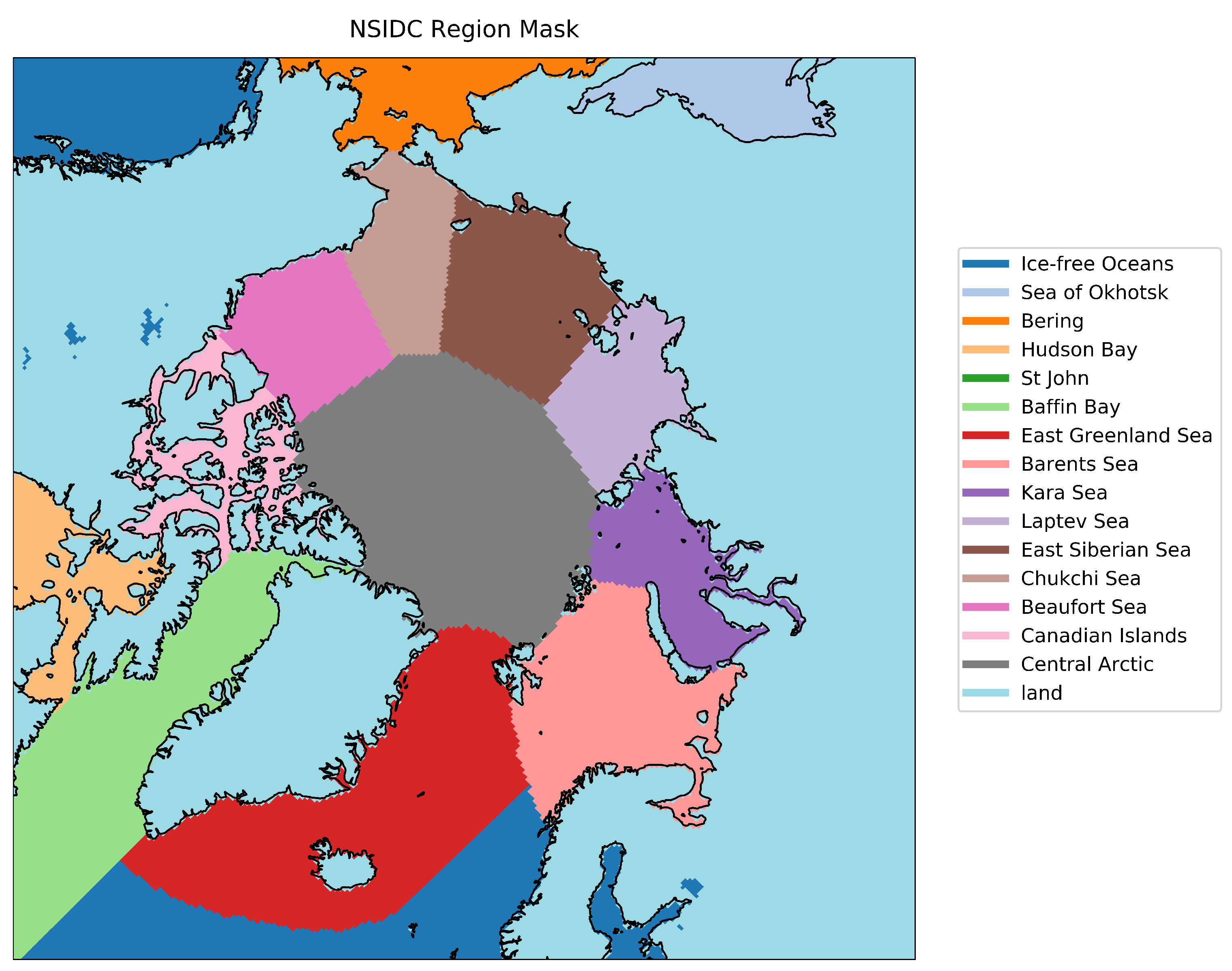
Cross validation is an important method to quantify the performance of the predictive behaviour of a given model. Such assessments quantify how a model will generalize to new or unseen data and is critical to prevent overfitting. The general principle of this method is to suppress a proportion of the data used to construct the model, and to use the suppressed data as an independent dataset to assess model performance. One such method is known as k-fold cross validation, where a dataset is split into a number of classes, known as folds, and for every fold, performance is assessed on a model constructed on the remaining folds. The performance metric from each fold is then averaged to denote an overall performance or cross-validation score. Underlying spatiotemporal correlations caused by a dataset comprised of adjacent incidents can introduce bias in cross-validation scores when using k-fold cross validation. This can result in overestimation of model performance [50]. Leave-one-group-out (LOGO) cross validation, where the permutation of split is defined using categorical data for grouping, was considered as a potential alternative cross-validation scheme with combinations of both the year, or the region (using the NSIDC regional mask, see Figure A1) in which an observation is considered as the category used for fold aggregation; however, this approach was rejected due to the formation of unbalanced classes which caused bias in metric aggregation during cross-validation assessment.

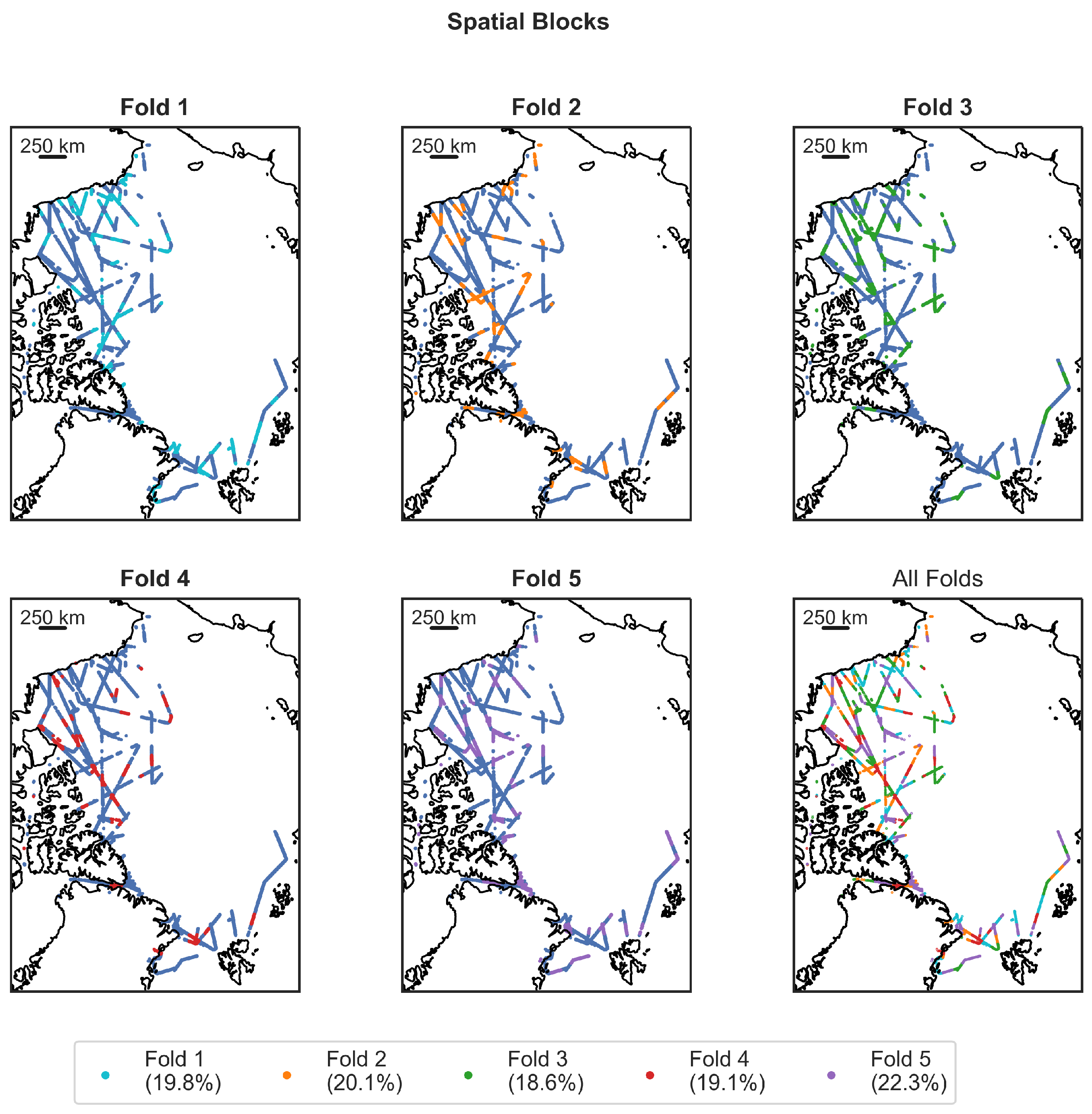
Instead, model performance was assessed using blocked k-fold cross validation, a scheme that is both respective of spatiotemporal correlations and allows for formation of balanced classes. A 100 km grid is constructed and overlain on the training data such that each incident is assigned a membership of a particular block. These blocks are then randomly aggregated to form some number of classes, such that the classes contain roughly equal numbers of training incidents, which are then used to determine the split permutation (Figure 5). Overall performance is then derived from a mean average of each performance metric as determined by each fold.

A forward-floating sequential feature-selection scheme was implemented to determine the optimal features to include in the model. The feature subset is iteratively constructed by assessing model performance through cross validation on initially each single feature, with the optimum feature then selected and additional features included on the same basis. The floating element describes the process where previously included features can be excluded or replaced at each round if this is found to improve model performance. Blue bands are excluded from modelling due to uncorrected Rayleigh scattering. To avoid overfitting from contextual features, some features, such as geolocation information and redundant orbit parameters, are not included in the feature-selection process. The features available for modelling were the camera angles Cf, Af, An, Aa, Ca for the red and NIR bands, solar zenith angle, relative azimuth angle for the aforementioned cameras, and ice-surface temperature (from MODIS). Presented in Figure 6 is the result of this feature-selection process. As hyperparameterisation affects the model implemented for feature selection ($\gamma$ is particularly sensitive to the number of input features) and, conversely, feature selection impacts the model implemented for hyperparameterisation, these two processes should not be thought of as two distinct steps which follow each-other, but rather as a concurrent process which converges on some combination of both features and defined hyperparameters for optimal trade off between bias and variance. In Figure 6 and Figure 7, we present this final model.

Model performance with increasing features plateaus after approximately eight features, with a maximum at 10 features. These 10 features selected for modelling are Aa, An, Ca (red channel), An, Af, Ca (NIR channel), solar zenith angle, relative azimuth angle for Ca and Cf, and ice-curface temperature.

The support vector regression (SVR) analysis chosen requires optimal tuning of the three hyperparameters, the cost function (C), the insensitive loss ($ϵ$), and the kernel parameter ($\gamma$), which together determine the shape of the hyperplane. It is, therefore, critical for the development of a successful model that appropriate hyperparameters are selected. Grid-search cross validation describes the process of computing model performance over a comprehensive range of hyperparameters, termed a grid. This process is performed over an initially coarse grid of several orders of magnitude (Figure 7) for each hyperparameter. Once the optimal order of magnitude for each hyperparameter is determined from the coarse grid, this process is then repeated on a finer grid to determine precisely the optimal combination of hyperparameters. Hyperparameters of C = 0.8, $ϵ$ = 0.4, $\gamma$ = 0.05 were selected.

Learning curves are common tools for quantifying bias–variance trade off in modelling, in order to prevent overfitting and to identify underfitting. The objective is to compare how well a particular model generalises to itself ($R^2$ train, or training score) compared with how well it generalises to unseen data ($R^2$ test, or cross-validation score) over an increasing fraction of the input data used for model construction. Convergence occurs at the point where our model has fully generalized to unseen data, indicating that overfitting has been avoided. The model performance at the point of convergence defines the potential extent of underfitting.

The learning curve of our model after selection of appropriate hyperparameters and features as described is presented in Figure 8, illustrating model performance (from blocked k-fold cross validation, where $k=5$) for two metrics ($R^2$, and MAE) for increasing training fractions in 10% increments of the available data, with shaded $\pm 1\sigma$ errors from aggregation of scores over folds. Whilst the training scores are better (towards 1 for $R^2$, towards 0 for MAE) for lower training fractions, the difference between the training and testing performance is sizeable, indicating an over-fit and poor generalisation to new data. As the training fraction increases, the difference between training scores and testing scores decreases and plateaus at similar values around 12,000 data points for both metrics.

The cross-validated performance of our model using the specified hyperparameters and features is given in

Table 3. A demonstration of cross-validation performance metrics for each fold and average performance for our selected model. Note that whilst the cross-validation assessment was performed subsequent to the Box–Cox transform on the output roughness, for this table, this transform was inverted on the calculated MAE so as to present errors which are intuitively meaningful.

Fold	${\mathit{R}}^2$ (Test)	${\mathit{R}}^2$ (Train)	MAE (m)
1	0.36	0.55	0.044
2	0.48	0.52	0.041
3	0.32	0.53	0.033
4	0.43	0.54	0.045
5	0.48	0.53	0.041
Mean	0.43	0.53	0.041

. The permutation of split for each fold in cross validation is illustrated in Figure 5. MAEs presented are transformed into the original parameter space and exhibit convergence towards the 3 cm error intrinsic to the IceBridge ATM.

Our processing chain was then applied to MISR imagery from 2000–2020 for April, in order to construct a multi-decadal pan-Arctic-surface-roughness archive. In applying our model, we flagged and removed any derived measurements of surface roughness where any feature of the input vector ${\mathit{x}}_{\mathit{i}}$ lies outside the range of the trained parameter space denoted by deviations of ±3$\sigma$.

3. Results

In this section, we present our derived roughness product at the swath level, as illustrated for three different surface types (smooth, rough, and transitional). The swath-level product is aggregated by month to a 1 km EASE-2 grid to generate an average product, and a regional and inter-annual comparison is presented. We begin with an outline of the aforementioned two production-level roughness products.

We demonstrate our swath-level product through illustration of three scenes, corresponding to three different roughness regimes.

Figure 9a shows a swath in the Russian Arctic, located in the Laptev and East Siberian Seas, traversing over the New Siberian Islands. This is a particular region of interest due to the observation of newly formed smooth sea ice and polynya, in addition to the coverage of fast ice and pack ice. This region along the Russian coast is often described as a sea-ice factory, as the prevailing northward currents and winds push the ice offshore and promote winter ice growth [51,52]. It should be noted that, due to the implementation of MOD29 for surface type classification, both open ocean and clouds are suppressed and so polynyas are not directly imaged but their extent can be inferred from the swath-level product, particularly after refreeze.

Figure 9b shows a swath in the East Greenland Sea between Nord and Svalbard, a region known for the prominence of drift ice, which contributes to a transition between smooth and rough surface morphologies of drift ice where the transpolar drift and local outflux of older ice from the North of Greenland converge [53,54,55] relating to declining multiyear ice cover. This scene intersects open ocean immediately off the coast north of Svalbard.

Figure 9c shows a swath over the Central Arctic, extending north of Ellesmere Island, traversing the rougher, thicker multi-year ice. Seasonal and interannual variability in the roughness patterns is controlled by the degree of coastal convergence, itself related to the prevailing wind patterns associated with the Arctic Oscillation [56,57]. This shows particularly prominent ridge features in the region adjacent to the coast of Ellesmere Island, in addition to textures consistent with some cloud contamination as the swath progresses northwards.

An example of the monthly gridded roughness product is provided in Figure 10 for April 2016, demonstrating the monthly gridded roughness (left), and the associated counts (top right), standard deviations (STD; middle left), and coefficients of variation (CoV; bottom right). The CoV is the ratio of the roughness STD over its mean value and is typically larger over regions undergoing rapid drift during the 30-day temporal-averaging period. Of note are distinct roughness morphologies related to convergence and divergence associated with the Beaufort gyre, smooth-ice formation in the Laptev and East Siberian sea, with increased roughness coincident with multi-year ice in the Central Arctic, and the low-arch system that formed in the Nares strait in spring 2016.

Missing data at high latitudes (north of ≈84°) is intrinsic to all products, due to the relatively narrow swath width of the MISR sensor combined with the 98° inclination of the Terra platform. Repeat reconnaissance is maximum in the region adjacent to this ‘pole-hole’, with decreasing observations associated with lower latitudes, as illustrated in Figure 9 top-right (count). Theoretical pan-Arctic coverage is achieved every three days; however, due to cloud cover and darkness, this is reduced to around seven days for practical purposes.

Using the April monthly averaged roughness product, we generated a multi-annual mask removing any values from all years which do not constitute a complete time record. We then implemented the NSIDC Regional Mask Figure A1 to define our regions of interest for analysis. Two assessments were made, the first presented is roughness distribution by region (

Table 4. A table showing surface-roughness distributions grouped by Arctic region, for April 2000–2020. Arctic regions are as defined in the NSIDC Regional Mask, illustrated in Figure A1.

Region	Roughness (m)
	Mean	STD	Minimum	25%	Median	75%	Maximum
Baffin Bay	0.105	0.033	0.010	0.081	0.100	0.124	0.447
Barents Sea	0.091	0.029	0.011	0.071	0.088	0.107	0.464
Beaufort Sea	0.120	0.026	0.016	0.104	0.118	0.134	0.356
Canadian Islands	0.129	0.032	0.018	0.108	0.126	0.146	0.457
Central Arctic	0.138	0.028	0.019	0.120	0.135	0.154	0.460
Chukchi Sea	0.117	0.028	0.018	0.099	0.116	0.132	0.404
East Greenland Sea	0.123	0.033	0.013	0.101	0.121	0.143	0.505
East Siberian Sea	0.115	0.026	0.020	0.100	0.113	0.127	0.345
Kara Sea	0.104	0.029	0.016	0.084	0.101	0.121	0.395
Laptev Sea	0.111	0.024	0.019	0.094	0.110	0.125	0.308

), the second roughness distribution by year (

Table 5. A table showing roughness distribution grouped by year, for April 2000–2020.

Year (April)	Roughness (m)
	Mean	STD	Minimum	25%	Median	75%	Maximum
2000	0.164	0.032	0.014	0.147	0.166	0.185	0.481
2001	0.147	0.030	0.018	0.131	0.150	0.164	0.489
2002	0.131	0.032	0.016	0.110	0.132	0.150	0.524
2003	0.120	0.029	0.015	0.102	0.119	0.136	0.469
2004	0.122	0.029	0.013	0.106	0.121	0.138	0.471
2005	0.119	0.027	0.012	0.102	0.121	0.136	0.491
2006	0.119	0.027	0.011	0.104	0.121	0.133	0.397
2007	0.108	0.027	0.013	0.090	0.107	0.123	0.464
2008	0.103	0.026	0.015	0.086	0.103	0.117	0.416
2009	0.114	0.027	0.013	0.097	0.114	0.131	0.467
2010	0.104	0.025	0.014	0.090	0.106	0.119	0.421
2011	0.120	0.028	0.012	0.104	0.121	0.134	0.488
2012	0.106	0.029	0.010	0.089	0.105	0.123	0.447
2013	0.108	0.025	0.013	0.092	0.108	0.122	0.455
2014	0.106	0.029	0.014	0.087	0.104	0.119	0.462
2015	0.114	0.028	0.015	0.096	0.112	0.129	0.458
2016	0.116	0.031	0.015	0.096	0.118	0.133	0.477
2017	0.112	0.030	0.016	0.091	0.112	0.130	0.507
2018	0.111	0.026	0.018	0.095	0.110	0.124	0.454
2019	0.110	0.029	0.010	0.091	0.109	0.126	0.490
2020	0.118	0.030	0.016	0.096	0.117	0.140	0.429

).

The roughest region on average (mean) in this study period is the Central Arctic, although the roughest observations are in the East Greenland Sea. This is consistent with the expected distribution of multi-year ice, which is more deformed and so rougher. Additionally towards the rougher end of the spectrum are the Canadian Islands. The smoothest region is the Barents sea, consistent with the expected distribution of smoother first-year ice. Towards the smoother end of the spectrum are the Kara Sea and Baffin Bay. This is consistent with the expected distribution of multi-year ice, which is more deformed and so rougher [58,59].

The roughest year in this study period was 2000, with average pan-Arctic roughness of 16.4 cm. The smoothest year was 2008 (10.3 cm).

4. Discussion

To demonstrate the validity of the derived product, we first evaluated our roughness product against independent LiDAR characterisations of surface roughness consistent with our training data. We selected four pre-IceBridge [35] aerial campaigns (22 March 2006, 24 March 2006, 25 March 2006, and 27 March 2006) for this purpose. Cross sections of coincident MISR-derived roughness swaths were extracted, where these were visually cloud-free and substantive intersection within $\pm 36$ h, and subsequently compared with observations of sea-ice surface roughness for several MISR-derived roughness scenes, as described in

Table 6. Comparative assessment of MISR-derived roughness against a roughness from independent pre-IceBridge (March 2006) aerial campaigns, where PMCC is product motion correlation coefficient, p < 0.001 for all scenes except Orbit 33341 where p < 0.005.

Orbit	Path	Count	Date	Time	Roughness (m)			PMCC
					Mean	Median	STD
33299	90	665	22 March 2006	23:08:21	0.105	0.103	0.027	0.71
33314	97	356	23 March 2006	23:51:36	0.097	0.095	0.012	0.64
33328	88	756	24 March 2006	22:55:59	0.127	0.125	0.024	0.74
33341	63	205	25 March 2006	20:21:29	0.233	0.235	0.035	0.20
33342	79	1259	25 March 2006	22:00:22	0.148	0.141	0.037	0.56
33370	61	95	27 March 2006	20:09:07	0.204	0.213	0.046	0.65

.

The scene with the greatest intersection is illustrated in Figure 11, which shows a scene in the Central Arctic, extending northwards from Greenland.

The line of section extends from fast ice immediately off the coast of Greenland (Figure 11, black) northwards to the edge of the MISR scene (Figure 11, green) traversing the oldest and roughest ice in the Arctic, and a prominent lead. Good agreement is demonstrated between derived roughness and pre-IceBridge-derived ground-truth surface-roughness observations, scene-by-scene comparisons between the predicted and observed surface roughness exhibit high correlation coefficients (Table 6).

We also evaluated our derived roughness product with known proxies of surface roughness on a pan-Arctic basis. As sea-ice surface roughness is known to be correlated with thickness (and age), a comparison between MISR-derived surface roughness and the AWI CS2-SMOS merged sea-ice thickness product was performed. Sea-ice thickness over the overlapping temporal interval 01–15 April 2011–2020 were aggregated by year onto an EASE-2 25 km grid and a roughness product for the same temporal window was generated; subsequently, a multi-year conservative mask was applied such that grid cells containing any missing data for any year were excluded from the comparison.

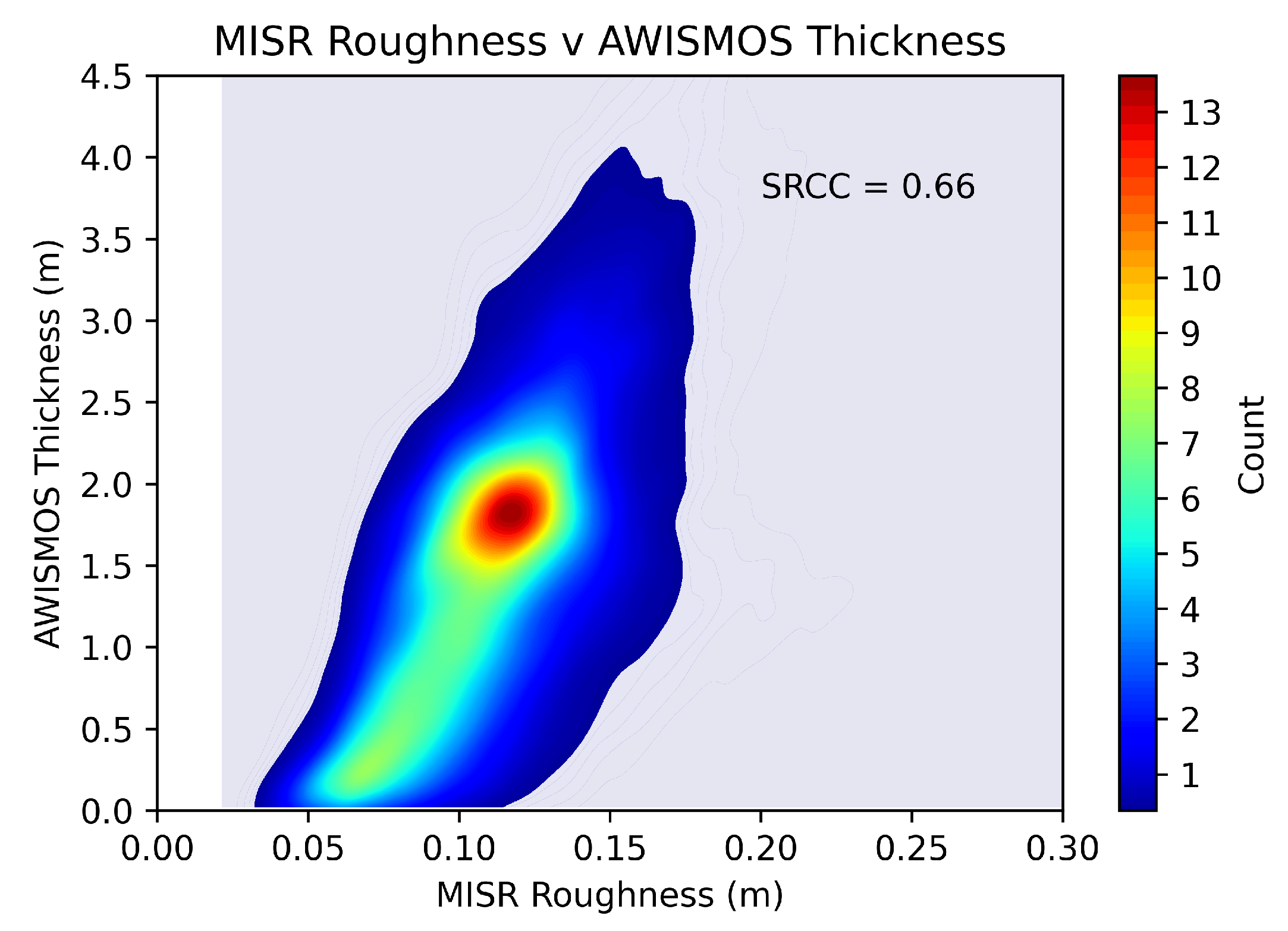
The overall correlation between the derived MISR roughness and AWI CS-2 SMOS-derived thickness is 0.66; the nature of this correlation is illustrated in Figure 12 as a bivariate distribution plot. In addition, the correlations between roughness and thickness exhibits regional and inter-annual variation.

Table 7. Spearman’s rank correlation coefficients (p < 0.001) between MISR-derived SIR and AWI CS-2 SMOS thickness by region. Correlations above this confidence interval are not reported.

	2011	2012	2013	2014	2015	2016	2017	2018	2019
Baffin Bay	0.81	0.59	0.36	0.69	0.83	0.67	0.58	0.5	0.52
East Greenland Sea	0.64	0.57	0.71	0.67	0.44	0.81	0.63	0.63	0.74
Barents Sea	0.68	0.39	0.7	0.49	0.55	0.57	0.23	0.59	0.49
Kara Sea	0.76	0.7	0.21	0.46	0.48	0.67	0.65	0.37	0.7
Laptev Sea	0.67	0.56	0.71	0.78	0.67	0.68	0.39	0.52	0.8
East Siberian Sea	0.51	0.35	0.21	0.17	0.63	0.25	0.65	0.07	0.44
Chukchi Sea	-	0.15	0.29	0.21	0.6	0.21	0.16	0.78	0.46
Beaufort Sea	0.27	0.57	0.43	0.64	0.42	0.53	−0.16	0.43	0.61
Canadian Islands	0.24	0.34	0.27	0.63	0.48	0.64	0.49	0.62	0.63
Central Arctic	0.55	0.87	0.68	0.86	0.83	0.85	0.77	0.6	0.82

illustrates these correlations by region (as defined by the regions as outlined in Figure A1) and two-dimensional scatter plots of a similar nature to Figure 12 for each region can be located in Figure A2.

Correlations between MISR-derived SIR and AWI CS-2 SMOS thickness are highest in the Central Arctic, and lowest in the East Siberian sea. This correlation between sea-ice thickness and roughness has long been established, as discussed in [2], and reflects the correlated nature of the age, thickness and ridging of the sea-ice surface.

5. Conclusions

In this study, we demonstrate that non-linear regression modelling of components of angular-reflectance signatures from the MISR instrument are correlated with measurements of surface roughness from laser altimetry, which can be used to generate a multi-decadal (2000–2020) novel roughness product, allowing for high-resolution (1.1 km) visualisation of convergence and divergence features (such as ridges and leads) and sea-ice formation. When re-gridded to a similar spatial and temporal resolution, such as AWI CS2-SMOS thickness, our derived roughness product is closely correlated (SRCC = 0.66, p < 0.001) with thickness.

Future extensions of this work include the application of this novel technique for the retrieval of Antarctic sea-ice surface roughness over the Greenland and Antarctic ice sheets but also for the broader characterisation of other textured surfaces such as lakes, and sand dunes. Such work should also focus on expanding the seasonality of this product, such as through the use of ICESat-II measurements of surface roughness for model generation, or the implementation of a regression scheme that yields probabilistic estimates of surface roughness, such as relevance vector machines [60], allowing extrapolation to lower solar zenith angles with quantifiable errors. As surface roughness provides preconditioning for summer-melt pond formation, which constitutes a crucial part of ice-albedo feedback, potential work could include applications related to sea-ice minimum extent forecasting. The combination of relatively high resolution and good coverage together with novel information on the roughness and thickness of the sea ice makes this product an ideal candidate to support operation needs for shipping in the ice-covered Arctic Ocean.

This work also highlights the need for a quantitative study on the comparative performance of operational cloud masks on the Terra platform for ice-covered surfaces.

References

1. Thomas, T. Characterization of surface roughness. Precis. Eng. 1981, 3, 97–104. [Google Scholar] [CrossRef]
2. Martin, T. Arctic Sea Ice Dynamics: Drifts and Ridging in Numerical Models and Observations; Alfred-Wegener-Institut für Polar-und Meeresforschung, University of Bremen: Bremen, Germany, 2007; Volume 563. [Google Scholar]
3. Segal, R.A.; Scharien, R.K.; Duerden, F.; Tam, C.L. The Best of Both Worlds: Connecting Remote Sensing and Arctic Communities for Safe Sea Ice Travel. Arctic 2020, 73, 461–484. [Google Scholar] [CrossRef]
4. Dammann, D.O.; Eicken, H.; Mahoney, A.R.; Saiet, E.; Meyer, F.J.; John, C. Traversing sea ice—Linking surface roughness and ice trafficability through SAR polarimetry and interferometry. IEEE J. Sel. Top. Appl. Earth Obs. Remote Sens. 2017, 11, 416–433. [Google Scholar] [CrossRef]
5. Martin, T.; Tsamados, M.; Schroeder, D.; Feltham, D.L. The impact of variable sea ice roughness on changes in Arctic Ocean surface stress: A model study. J. Geophys. Res. Ocean. 2016, 121, 1931–1952. [Google Scholar] [CrossRef] [Green Version]
6. Petty, A.A.; Tsamados, M.C.; Kurtz, N.T. Atmospheric form drag coefficients over Arctic sea ice using remotely sensed ice topography data, spring 2009–2015. J. Geophys. Res. Earth Surf. 2017, 122, 1472–1490. [Google Scholar] [CrossRef] [Green Version]
7. Tsamados, M.; Feltham, D.L.; Schroeder, D.; Flocco, D.; Farrell, S.L.; Kurtz, N.; Laxon, S.W.; Bacon, S. Impact of variable atmospheric and oceanic form drag on simulations of Arctic sea ice. J. Phys. Oceanogr. 2014, 44, 1329–1353. [Google Scholar] [CrossRef] [Green Version]
8. Petrich, C.; Eicken, H.; Polashenski, C.M.; Sturm, M.; Harbeck, J.P.; Perovich, D.K.; Finnegan, D.C. Snow dunes: A controlling factor of melt pond distribution on Arctic sea ice. J. Geophys. Res. Ocean. 2012, 117, C9. [Google Scholar] [CrossRef]
9. Landy, J.C.; Ehn, J.K.; Barber, D.G. Albedo feedback enhanced by smoother Arctic sea ice. Geophys. Res. Lett. 2015, 42, 10–714. [Google Scholar] [CrossRef]
10. Landy, J.C.; Petty, A.A.; Tsamados, M.; Stroeve, J.C. Sea ice roughness overlooked as a key source of uncertainty in CryoSat-2 ice freeboard retrievals. J. Geophys. Res. Ocean. 2020, 125, e2019JC015820. [Google Scholar] [CrossRef]
11. Leberl, F.W. A review of: “Microwave Remote Sensing—Active and Passive”. By F. T. Ulaby. R. K. Moore and A. K. Fung. (Reading, Massachusetts: Addison-Wesley, 1981 and 1982.) Volume I: Microwave Remote Sensing Fundamentals and Radiometry. [Pp. 473.] Volume II: Radar Remote Sensing and Surface Scattering and Emission Theory. [Pp. 628.]. Int. J. Remote Sens. 1984, 5, 463–466. [Google Scholar] [CrossRef]
12. Lindell, D.; Long, D. Multiyear arctic ice classification using ASCAT and SSMIS. Remote Sens. 2016, 8, 294. [Google Scholar] [CrossRef] [Green Version]
13. Girard-Ardhuin, F.; Ezraty, R. Enhanced Arctic Sea Ice Drift Estimation Merging Radiometer and Scatterometer Data. IEEE Trans. Geosci. Remote Sens. 2012, 50, 2639–2648. [Google Scholar] [CrossRef] [Green Version]
14. Kwok, R.; Rignot, E.; Holt, B.; Onstott, R. Identification of sea ice types in spaceborne synthetic aperture radar data. J. Geophys. Res. Ocean. 1992, 97, 2391–2402. [Google Scholar] [CrossRef] [Green Version]
15. Casey, J.A.; Beckers, J.; Busche, T.; Haas, C. Towards the retrieval of multi-year sea ice thickness and deformation state from polarimetric C- and X-band SAR observations. In Proceedings of the 2014 IEEE Geoscience and Remote Sensing Symposium, Quebec City, QC, Canada, 13–18 July 2014; pp. 1190–1193. [Google Scholar] [CrossRef]
16. Karvonen, J.; Simila, M.; Heiler, I. Ice thickness estimation using SAR data and ice thickness history. In Proceedings of the IGARSS 2003. 2003 IEEE International Geoscience and Remote Sensing Symposium, Toulouse, France, 21–25 July 2003; Volume 1, pp. 74–76. [Google Scholar] [CrossRef]
17. Daida, J.; Onstott, R.; Bersano-Begey, T.; Ross, S.; Vesecky, J. Ice roughness classification and ERS SAR imagery of Arctic sea ice: Evaluation of feature-extraction algorithms by genetic programming. In Proceedings of the IGARSS ’96. 1996 International Geoscience and Remote Sensing Symposium, Lincoln, NE, USA, 31 May 1996; Volume 3, pp. 1520–1522. [Google Scholar] [CrossRef]
18. Segal, R.A.; Scharien, R.K.; Cafarella, S.; Tedstone, A. Characterizing winter landfast sea-ice surface roughness in the Canadian Arctic Archipelago using Sentinel-1 synthetic aperture radar and the Multi-angle Imaging SpectroRadiometer. Ann. Glaciol. 2020, 61, 284–298. [Google Scholar] [CrossRef]
19. Farrell, S.L.; Duncan, K.; Buckley, E.M.; Richter-Menge, J.; Li, R. Mapping Sea Ice Surface Topography in High Fidelity with ICESat-2. Geophys. Res. Lett. 2020, 47, e2020GL090708. [Google Scholar] [CrossRef]
20. Nolin, A.W.; Fetterer, F.M.; Scambos, T.A. Surface roughness characterizations of sea ice and ice sheets: Case studies with MISR data. IEEE Trans. Geosci. Remote Sens. 2002, 40, 1605–1615. [Google Scholar] [CrossRef] [Green Version]
21. Nolin, A.W.; Payne, M.C. Classification of glacier zones in western Greenland using albedo and surface roughness from the Multi-angle Imaging SpectroRadiometer (MISR). Remote Sens. Environ. 2007, 107, 264–275. [Google Scholar] [CrossRef]
22. Nolin, A.W.; Mar, E. Arctic sea ice surface roughness estimated from multi-angular reflectance satellite imagery. Remote Sens. 2019, 11, 50. [Google Scholar] [CrossRef] [Green Version]
23. Studinger, M. IceBridge ATM L2 Icessn Elevation, Slope, and Roughness, Version 2; NSIDC: Boulder, CO, USA, 2014; Updated 2020. [Google Scholar] [CrossRef]
24. Ricker, R.; Hendricks, S.; Kaleschke, L.; Tian-Kunze, X.; King, J.; Haas, C. A weekly Arctic sea-ice thickness data record from merged CryoSat-2 and SMOS satellite data. Cryosphere 2017, 11, 1607–1623. [Google Scholar] [CrossRef] [Green Version]
25. Studinger, M. IceBridge ATM L1B Qfit Elevation and Return Strength, Version 1; NSIDC: Boulder, CO, USA, 2010; Updated 2013. [Google Scholar] [CrossRef]
26. Studinger, M. IceBridge ATM L1B Elevation and Return Strength, Version 2; NSIDC: Boulder, CO, USA, 2013; Updated 2020. [Google Scholar] [CrossRef]
27. NASA/LARC/SD/ASDC. MISR Level 1B2 Ellipsoid Data V003. 2007. Available online: https://asdc.larc.nasa.gov/project/MISR/MI1B2E_3 (accessed on 1 January 2022).
28. NASA/LARC/SD/ASDC. MISR Geometric Parameters V002. 2008. Available online: https://asdc.larc.nasa.gov/project/MISR/MIB2GEOP_2 (accessed on 1 January 2022).
29. NASA/LARC/SD/ASDC. MISR Level 2 TOA/Cloud Classifier Parameters V003. 2008. Available online: https://asdc.larc.nasa.gov/project/MISR/MIL2TCCL_3 (accessed on 1 January 2022).
30. NASA/LARC/SD/ASDC. MISR Level 2 TOA/Cloud Height and Motion Parameters V001. 2012. Available online: https://asdc.larc.nasa.gov/project/MISR/MIL2TCSP_1 (accessed on 1 January 2022).
31. Hall, D.K.; Riggs, G. MODIS/Terra Sea Ice Extent 5-Min L2 Swath 1km, Version 6; NSIDC: Boulder, CO, USA, 2015. [Google Scholar] [CrossRef]
32. MODIS Science Team. MODIS/Terra Geolocation Fields 5-Min L1A Swath 1 km, Version 6; L1 and Atmosphere Archive and Distribution System: Greenbelt, MD, USA, 2015. [CrossRef]
33. MCST Team. MODIS/Terra Calibrated Radiances 5-Min L1B Swath 1 km, Version 6; L1 and Atmosphere Archive and Distribution System: Greenbelt, MD, USA, 2015. [CrossRef]
34. Tschudi, M.; Meier, W.N.; Stewart, J.S.; Fowler, C.; Maslanik, J. Polar Pathfinder Daily 25 km EASE-Grid Sea Ice Motion Vectors, Version 4; NSIDC: Boulder, CO, USA, 2019. [Google Scholar] [CrossRef]
35. Studinger, M. Pre-IceBridge ATM L1B Qfit Elevation and Return Strength, Version 1; NSIDC: Boulder, CO, USA, 2012. [Google Scholar] [CrossRef]
36. MISR Toolkit. Available online: https://github.com/nasa/MISR-Toolkit (accessed on 1 January 2022).
37. Muller, J.P.; Mandanayake, A.; Moroney, C.; Davies, R.; Diner, D.J.; Paradise, S. MISR stereoscopic image matchers: Techniques and results. IEEE Trans. Geosci. Remote Sens. 2002, 40, 1547–1559. [Google Scholar] [CrossRef] [Green Version]
38. Mueller, K.; Moroney, C.; Jovanovic, V.; Garay, M.; Muller, J.; Di Girolamo, L.; Davies, R. MISR Level 2 Cloud Product Algorithm Theoretical Basis; JPL Tech. Doc. JPL D-73327; Jet Propulsion Laboratory, California Institute of Technology: Pasadena, CA, USA, 2013. [Google Scholar]
39. Horvath, A. Improvements to MISR stereo motion vectors. J. Geophys. Res. 2013, 118, 5600–5620. [Google Scholar] [CrossRef]
40. Zhan, Y.; Di Girolamo, L.; Davies, R.; Moroney, C. Instantaneous Top-of-Atmosphere Albedo Comparison between CERES and MISR over the Arctic. Remote Sens. 2018, 10, 1882. [Google Scholar] [CrossRef] [Green Version]
41. Hutchison, K.D.; Mahoney, R.L.; Vermote, E.F.; Kopp, T.J.; Jackson, J.M.; Sei, A.; Iisager, B.D. A geometry-based approach to identifying cloud shadows in the VIIRS cloud mask algorithm for NPOESS. J. Atmos. Ocean. Technol. 2009, 26, 1388–1397. [Google Scholar] [CrossRef] [Green Version]
42. Shi, T.; Yu, B.; Clothiaux, E.E.; Braverman, A.J. Daytime Arctic Cloud Detection Based on Multi-Angle Satellite Data with Case Studies. J. Am. Stat. Assoc. 2008, 103, 584–593. [Google Scholar] [CrossRef] [Green Version]
43. Kharbouche, S.; Muller, J.P. Sea Ice Albedo from MISR and MODIS: Production, Validation, and Trend Analysis. Remote Sens. 2019, 11, 9. [Google Scholar] [CrossRef] [Green Version]
44. Lee, S.; Stroeve, J.; Tsamados, M.; Khan, A.L. Machine learning approaches to retrieve pan-Arctic melt ponds from visible satellite imagery. Remote Sens. Environ. 2020, 247, 111919. [Google Scholar] [CrossRef]
45. Drucker, H.; Burges, C.J.; Kaufman, L.; Smola, A.; Vapnik, V. Support vector regression machines. Adv. Neural Inf. Process. Syst. 1997, 9, 155–161. [Google Scholar]
46. Mazzoni, D.; Garay, M.J.; Davies, R.; Nelson, D. An operational MISR pixel classifier using support vector machines. Remote Sens. Environ. 2007, 107, 149–158. [Google Scholar] [CrossRef]
47. Durbha, S.S.; King, R.L.; Younan, N.H. Support vector machines regression for retrieval of leaf area index from multiangle imaging spectroradiometer. Remote Sens. Environ. 2007, 107, 348–361. [Google Scholar] [CrossRef]
48. Chang, C.C.; Lin, C.J. LIBSVM: A Library for Support Vector Machines. ACM Trans. Intell. Syst. Technol. 2011, 2, 27:1–27:27. Available online: http://www.csie.ntu.edu.tw/~cjlin/libsvm (accessed on 1 January 2022). [CrossRef]
49. Awad, M.; Khanna, R. Efficient Learning Machines: Theories, Concepts, and Applications for Engineers and System Designers, 1st ed.; Apress: New York, NY, USA, 2015. [Google Scholar]
50. Roberts, D.R.; Bahn, V.; Ciuti, S.; Boyce, M.S.; Elith, J.; Guillera-Arroita, G.; Hauenstein, S.; Lahoz-Monfort, J.J.; Schröder, B.; Thuiller, W.; et al. Cross-validation strategies for data with temporal, spatial, hierarchical, or phylogenetic structure. Ecography 2017, 40, 913–929. [Google Scholar] [CrossRef] [Green Version]
51. Itkin, P.; Krumpen, T. Winter sea ice export from the Laptev Sea preconditions the local summer sea ice cover and fast ice decay. Cryosphere 2017, 11, 2383–2391. [Google Scholar] [CrossRef] [Green Version]
52. Cornish, S.; Johnson, H.; Mallett, R.; Dörr, J.; Kostov, Y.; Richards, A.E. Rise and fall of ice production in the Arctic Ocean’s ice factories. Earth Space Sci. Open Arch. 2021. [Google Scholar] [CrossRef]
53. Belter, H.J.; Krumpen, T.; von Albedyll, L.; Alekseeva, T.A.; Birnbaum, G.; Frolov, S.V.; Hendricks, S.; Herber, A.; Polyakov, I.; Raphael, I.; et al. Interannual variability in Transpolar Drift summer sea ice thickness and potential impact of Atlantification. Cryosphere 2021, 15, 2575–2591. [Google Scholar] [CrossRef]
54. Wang, Y.; Bi, H.; Liang, Y. A Satellite-Observed Substantial Decrease in Multiyear Ice Area Export through the Fram Strait over the Last Decade. Remote Sens. 2022, 14, 2562. [Google Scholar] [CrossRef]
55. Babb, D.G.; Galley, R.J.; Howell, S.E.; Landy, J.C.; Stroeve, J.C.; Barber, D.G. Increasing Multiyear Sea Ice Loss in the Beaufort Sea: A New Export Pathway for the Diminishing Multiyear Ice Cover of the Arctic Ocean. Geophys. Res. Lett. 2022, 49, e2021GL097595. [Google Scholar] [CrossRef]
56. Kwok, R. Sea ice convergence along the Arctic coasts of Greenland and the Canadian Arctic Archipelago: Variability and extremes (1992–2014). Geophys. Res. Lett. 2015, 42, 7598–7605. [Google Scholar] [CrossRef]
57. Mallett, R.; Stroeve, J.; Cornish, S.; Crawford, A.; Lukovich, J.; Serreze, M.; Barrett, A.; Meier, W.; Heorton, H.; Tsamados, M. Record winter winds in 2020/21 drove exceptional Arctic sea ice transport. Commun. Earth Environ. 2021, 2, 149. [Google Scholar] [CrossRef]
58. Duncan, K.; Farrell, S.L. Determining Variability in Arctic Sea Ice Pressure Ridge Topography with ICESat-2. Geophys. Res. Lett. 2022, 49, e2022GL100272. [Google Scholar] [CrossRef]
59. Castellani, G.; Lüpkes, C.; Hendricks, S.; Gerdes, R. Variability of A rctic sea-ice topography and its impact on the atmospheric surface drag. J. Geophys. Res. Ocean. 2014, 119, 6743–6762. [Google Scholar] [CrossRef]
60. Tipping, M.E. Sparse Bayesian learning and the relevance vector machine. J. Mach. Learn. Res. 2001, 1, 211–244. [Google Scholar]
Figure 1. A schematic of the MISR instrument, illustrating near-simultaneous acquisition of multi-angular reflectance, shown here as referenced to an ellipsoid. The time interval between ‘Time 0’ and ‘Time 1’ (representing the Cf and Ca bands, respectively) is approximately five minutes.
Remotesensing 14 06249 g001
Figure 2. An illustration of the different cloud masks (a) SDCM, (b) ASCM, (c) SVC, (d) MOD29, (e) MODIS-derived cloud shadow mask after [41], (f) MOD35; for Orbit O054627 Blocks 20–23 around Svalbard. Pixels designated as cloud free from each mask are displayed; however, only (c) and (d) actually implement a sea-ice classifier. For (a): 4 = Near Surface High Confidence, 3 = Near Surface Low Confidence, 2 = Cloud Low Confidence, 1 = Cloud High Confidence, 0 = No Retrieval (considered clear); (b): 4 = Clear High Confidence, 3 = Clear Low Confidence, 2 = Cloud Low Confidence, 1 = Cloud High Confidence, 0 = No Retrieval (considered cloud). In all cases, magenta denotes a high-confidence positive (considered cloud-free) retrieval, blue a low-confidence positive retrieval, purple a positive retrieval with no associated confidence interval presented, and red no retrieval considered positive. WGS 84 / NSIDC EASE-Grid 2.0 North. Generated using Cartopy and Matplotlib.
Remotesensing 14 06249 g002
Figure 3. A process diagram illustrating the workflow method used in model generation. Note that the model selection, feature selection, and hyper-parameterisation constitutes an iterative process that converges on a final hyper-parameterised model and feature subset via cross validation and bias-variance analysis.
Remotesensing 14 06249 g003
Figure 4. (left) PDFs of elevation used to characterise surface roughness used in training, (right) within-MISR pixel footprint of elevation measurements. N is the total number of elevation shots within a footprint; σ is the standard deviation of the elevation measurements, or roughness.
Remotesensing 14 06249 g004
Figure 5. A map demonstrating the permutation of split in each fold for five-fold block k-fold cross validation, using a 100 km block size. WGS 84/NSIDC EASE-Grid 2.0 North. Generated using Cartopy and Matplotlib.
Remotesensing 14 06249 g005
Figure 6. Model performance is shown for increasing numbers of features through successive iterations of our forward-floating sequential feature-selection scheme. The shaded region denotes ± 1 σ error from fold aggregation. The highest cross-validation performance was found for 10 features, although there was no increase in performance with increasing features, which plateaued after approximately seven features.
Remotesensing 14 06249 g006
Figure 7. A coarse grid search cross-validation scheme implemented using blocked k-fold cross validation. The example shown varies both C and γ for ϵ = 0.4. The coarse hyper parameters are denoted by the lowest CV scores at C = 1, γ = 0.1.
Remotesensing 14 06249 g007
Figure 8. Learning curves for our regression model at specified hyperparameters and features, for the coefficient of determination R 2 (left) and mean absolute error (right). Demonstrates training and testing performance (from blocked k-fold cross validation, where k = 5 ) for increasing training fractions in 10% increments. Highlighted regions demonstrate ± 1 σ errors from averaging folds. Performance of testing and training scores exhibits convergence for increasing training fractions. MAE scores are in the transformed feature space (Box–Cox power transformation).
Remotesensing 14 06249 g008
Figure 9. A swath-level product (left) for three different orbits which illustrates (a) a smooth, (b) an intermediate, and (c) a rough scene. For each scene, a histogram (right, bottom) of sea-ice surface roughness and summary statistics are provided (right, middle) in addition to a pan-Arctic map illustrating the location of the scene. Dates and times within the summary statistical table refer to the start of the given orbit. WGS 84/NSIDC EASE-Grid 2.0 North. Generated using Cartopy and Matplotlib.
Remotesensing 14 06249 g009aRemotesensing 14 06249 g009b
Figure 10. A sample monthly aggregated roughness product for April 2016; mean roughness (left); number of observations (top right); standard deviation of samples (middle right); coefficient of variation (bottom right), where CoV = standard deviation of roughness/mean roughness. WGS 84/NSIDC EASE-Grid 2.0 North. Generated using Cartopy and Matplotlib.
Remotesensing 14 06249 g010
Figure 11. Swath-level roughness scene with an overlain intersecting IceBridge flight path, and a line of section. For each scene, a histogram (right, bottom) of sea-ice surface roughness and summary statistics are provided (right, middle) in addition to a pan-Arctic map illustrating the location of the scene. Dates and times within the summary-statistics table refer to the start of a given orbit. WGS 84/NSIDC EASE-Grid 2.0 North. Generated using Cartopy and Matplotlib.
Remotesensing 14 06249 g011
Figure 12. Two-dimensional scatter plot shows a bivariate distribution between MISR-derived roughness (m) and AWI CS-2 SMOS merged thickness (m) for 01–15 April 2011–2020 and 25 km resolution. Count density refers to measurements over a 300 × 300 grid over the presented range (per 1.5 cm of thickness and per mm of roughness). The opaque shaded region represents 95% of the range, contours for the remaining percentiles are at single increments, and the valid bounds in light blue. Spearman’s rank correlation coefficient (SRCC) between derived MISR roughness and AWI CS-2 SMOS thickness is 0.66 (p < 0.001).
Remotesensing 14 06249 g012