Article

Dark Spot Detection from SAR Images Based on Superpixel Deeper Graph Convolutional Network

1
School of Remote Sensing and Information Engineering, Wuhan University, Wuhan 430079, China
2
Hubei Luojia Laboratory, Wuhan 430070, China
3
College of Global Change and Earth System Science, Beijing Normal University, Beijing 100875, China
*
Author to whom correspondence should be addressed.
Remote Sens. 2022, 14(21), 5618; https://doi.org/10.3390/rs14215618
Submission received: 19 September 2022 / Revised: 19 October 2022 / Accepted: 3 November 2022 / Published: 7 November 2022
(This article belongs to the Special Issue Reinforcement Learning Algorithm in Remote Sensing)

Abstract

:
Synthetic Aperture Radar (SAR) is the primary equipment used to detect oil slicks on the ocean’s surface. On SAR images, oil spill regions, as well as other places impacted by atmospheric and oceanic phenomena such as rain cells, upwellings, and internal waves, appear as dark spots. Dark spot detection is typically the initial stage in the identification of oil spills. Because the identified dark spots are oil slick candidates, the quality of dark spot segmentation will eventually impact the accuracy of oil slick identification. Although certain sophisticated deep learning approaches employing pixels as primary processing units work well in remote sensing image semantic segmentation, finding some dark patches with weak boundaries and small regions from noisy SAR images remains a significant difficulty. In light of the foregoing, this paper proposes a dark spot detection method based on superpixels and deeper graph convolutional networks (SGDCNs), with superpixels serving as processing units. The contours of dark spots can be better detected after superpixel segmentation, and the noise in the SAR image can also be smoothed. Furthermore, features derived from superpixel regions are more robust than those derived from fixed pixel neighborhoods. Using the support vector machine recursive feature elimination (SVM-RFE) feature selection algorithm, we obtain an excellent subset of superpixel features for segmentation to reduce the learning task difficulty. After that, the SAR images are transformed into graphs with superpixels as nodes, which are fed into the deeper graph convolutional neural network for node classification. SGDCN leverages a differentiable aggregation function to aggregate the node and neighbor features to form more advanced features. To validate our method, we manually annotated six typical large-scale SAR images covering the Baltic Sea and constructed a dark spot detection dataset. The experimental results demonstrate that our proposed SGDCN is robust and effective compared with several competitive baselines. This dataset has been made publicly available along with this paper.

1. Introduction

Among all the various kinds of marine pollution, oil pollution ranks first in terms of frequency of occurrence, extent of distribution, and degree of harm [1]. The pollution of offshore waters caused by oil spills continues to occupy the attention of researchers in many countries [2]. In particular, developed countries are investing a great deal of money in establishing oil spill monitoring systems to patrol, inspect, and manage offshore economic zones and territorial waters [3,4]. Synthetic Aperture Radar (SAR), which has the ability to penetrate clouds and fog and can work all day, is presently the most effective tool for oil pollution detection [1,5]. As oil spills on the sea surface cause the attenuation of the Bragg waves and reduce the roughness of the sea surface, the oil film generally appears as dark spots on SAR images [6]. However, some atmospheric and oceanic phenomena, such as upwelling, ocean internal waves, rain cells, and low winds, also appear as dark spots on SAR images, which are called “lookalikes”, making it difficult to distinguish them from dark spots caused by oil spills [7]. The purpose of oil spills detection is to discriminate between oily dark spots and lookalikes on SAR images. Typically, the traditional oil spill detection process using SAR satellite images is divided into three stages: (1) dark spot segmentation, (2) feature extraction, and (3) dark spot classification [7]. Dark spot detection is the first and most important step for oil spill detection, aiming to accurately segment all dark spots in SAR images, including real oil spills and lookalikes. The quality of feature extraction and, ultimately, the accuracy of dark spot classification are both affected by dark spot segmentation [8]. Any oil spills that are missed during the dark spot detection process will never be retrieved in the subsequent two phases. As a result, dark spot segmentation is critical for detecting oil spills.
There have been many studies pertaining to dark spot detection of oil spills using SAR, from simple to complex, which can be divided into three categories: (1) threshold-based approaches, (2) machine learning algorithms, and (3) deep learning algorithms. Threshold-based techniques are distinguished by their simplicity and rapid computation speed, and they typically need post-processing [9]. Since a single-scale threshold segmentation technique did not perform well in segmenting both large and small regions, Solberg et al. [10] proposed a multi-scale adaptive threshold segmentation method, which first created an image pyramid and then applied a threshold segmentation algorithm to each level of the pyramid to segment dark spots of different sizes. Shu et al. [7] developed a spatial density threshold method for automated dark spot detection, which used the kernel density to evaluate each potential background pixel after threshold segmentation to obtain the true dark spot pixel. Chehresa et al. [9] used a three-step strategy to detect dark spots that included image augmentation, Otsu thresholding, and post-processing. Compared with threshold-based approaches, machine learning (ML) algorithms are more popular in remote sensing image processing. Topouzelis et al. [11] proposed a simple recurrent neural network that takes the pixel to be segmented and four adjacent pixels as network input, which showed better performance in detecting dark formations. Taravat et al. [12] developed a new dark spot detection approach from the combination of a Weibull multiplicative model and a pulse-coupled neural network, which proved to be fast, robust, and effective. Lang et al. [13] designed three features suitable for dark spot segmentation: gray-scale features, geometric features, and texture features, which were then fed into a Multilayer Perceptron (MLP) for dark spot segmentation. With the development of artificial intelligence, dark spot detection methods based on deep learning have emerged in recent years. Xu et al. [14] presented a fully connected continuous conditional random field with stochastic cliques for dark spot detection on SAR images and proved its robustness against speckle noise. Guo et al. [15] suggested using the Segnet semantic segmentation model to detect dark spots on SAR images, and experiments showed that it is more effective than fully convolutional networks (FCN) [15,16] under fuzzy boundary and high noise conditions. Yekeen et al. [17] used a Mask Region-based Convolutional Neural Network (Mask R-CNN) [18] for oily instance segmentation and proved that it outperformed traditional machine learning models and semantic segment deep learning models. Based on VGG-16 [19], Zeng and Wang [20] developed a relatively deep convolutional neural network (DCNN) for oily dark spot detection, which outperformed traditional complex ML classifiers. To solve the label imbalance problem, Basit et al. [21] introduced a new loss function called “Gradient Profile” (GP) loss, which can significantly improve oily dark spot detection performance. Recently, Zhu et al. [22] developed an oil spill contextual and boundary-supervised detection network (CBD-Net) for detecting oily dark spots, which can improve the internal consistency of dark spot regions by using one spatial and channel squeeze excitation (scSE) block. In addition, they proposed a joint loss function for dealing with the fuzzy boundary problem of dark patches in SAR images.
Although the above methods employ different strategies to improve the performance of dark spot detection, the results are unsatisfactory in some complex sea areas with high noise and weak boundaries. Some researchers have demonstrated that superpixel segmentation techniques may be used in conjunction with some convolutional neural networks (CNNs) to improve image segmentation performance [23,24]. With the advancement of artificial intelligence technology in recent years [25], several researchers have begun to design more general deep learning algorithms, such as graph neural networks (GNNs), for processing non-Euclidean data [26,27]. Based on the above two techniques, this paper proposes a dark spot segmentation method combining GNNs and superpixel segmentation, which can improve the segmentation performance of dark spots with weak borders and small regions. This method begins by decomposing SAR images into superpixel blocks, which is employed as the fundamental processing units. Subsequently, the images are transformed into graphs with superpixels as nodes, which are fed into a graph neural network for node classification. This strategy can significantly reduce memory usage. After superpixel segmentation, dark spot boundaries can be detected more easily in the image. Simultaneously, superpixels can smooth out speckle noise in SAR images. Compared with existing pixel-based CNN algorithms and machine learning approaches, our method considerably improves dark spot segmentation performance. The details and experimental results of our method are introduced later in this paper.
The contributions of this paper are as follows: (1) For the first time, the deeper graph convolutional network is used for dark spot segmentation on SAR images. Compared with the existing pixel-based dark spot segmentation methods, this method can better handle the noise of SAR images and detect the boundaries of dark spots. The improved performance of dark spot segmentation will be more helpful for subsequent oil spill detection. (2) This work publishes a dark spot detection dataset to aid future dark spot detection research.
The remainder of this paper is structured as follows: Section 2 describes the study region and data used in this paper. Section 3 introduces our proposed dark spot detection method in detail, including images to graphs transformation, feature extraction, feature selection, and a GNN. Section 4 presents the research results, and Section 5 discusses the practicality of our proposed method and its limitations. Finally, Section 6 presents our conclusions and future directions of work.

2. Data and Study Region

Six Advanced Synthetic Aperture Radar (ASAR) products from the Envisat satellite were used to demonstrate the efficacy of the method proposed in this paper. The Envisat ASAR was developed by the European Space Agency (ESA) and operated in the C band in a wide variety of modes. The wide swath mode (WSM) in VV polarization that we used in our method is a one-of-a-kind instrument for detecting oil slicks on the ocean surface because it provides an excellent combination of wide coverage and radiometric quality [28]. In this mode, the incident angle of the acquired images ranges from 15 to 45°, the resolution is 150 m, and the swath is 405 km [28]. Inevitably, there may also be some brightness effects between subswaths of the image acquired in wide swath mode, which may hinder the detection of oil slicks. To solve this problem, Najoui et al. [29] applied a semi-linear model. As shown in Figure 1, the images we used cover most of the Baltic Sea, which is an important waterway in Northern Europe. The marine environment and coastal ecology of this ocean are constantly threatened by oil discharges from ships [30]. The SAR images used in this paper contain dark spots of various shapes and sizes, which are manually marked to form a dataset for dark spot detection. This dataset has been made publicly available alongside this paper (https://drive.google.com/drive/folders/12UavrntkDSPrItISQ8iGefXn2gIZHxJ6?usp=sharing, accessed on 4 June 2021).

3. Method

As illustrated in Figure 2, the dark spot detection method we propose consists of three steps: (1) image to graph structure conversion, (2) feature extraction and selection, and (3) graph node classification. The following sections go over the specifics of each step.

3.1. Conversion of the Image to Graph Structures

Before conversion, SAR images need to be preprocessed. Typically, this process includes radiometric calibration, reprojection, speckle filter, and masking out the land. We used the sentinel application platform (SNAP), which is a common architecture for ESA Toolboxes, for preprocessing [31]. For speckle filtering, a 3 × 3 Lee filter was chosen. The Lee filter has proved to be a very successful filter in the image processing of oil spill detection and has been used numerous times [32]. After preprocessing, SAR images are segmented into superpixel blocks. Some researchers have indicated that the features calculated from superpixel regions are more robust than those from fixed pixel neighborhoods [33]. Furthermore, Konik and Bradtke [30] showed that smooth SAR images or gradient images with obvious boundaries can significantly increase the accuracy of determining the outlines of dark spots. In this paper, we employ the Bayesian Adaptive Superpixel Segmentation approach (BASS) for superpixel segmentation, which is the state-of-the-art method that enables massive parallelization, and can be implemented on GPU [23]. After superpixel segmentation, pixels are grouped into homogeneous regions, reducing the number of items to be processed and thus significantly reducing the computational burden [34]. On the other hand, the shape, size, and number of adjacent superpixels are also changed. To process them efficiently, adjacent superpixels are connected, and images are transformed into graph structures with superpixels as nodes. Figure 3 shows this conversion, which follows this order: (1) each superpixel is treated as a node of the graph, and its center is calculated; (2) the centers of adjacent superpixels are connected, and the entire image is transformed into a single non-Euclidean structure graph; and (3) all nodes representing the land area are removed from the graph, as are the edges connected to them. Following conversion, each image is converted into a graph structure with at least one subgraph.

3.2. Feature Extraction and Feature Selection

In previous studies, feature extraction was mostly utilized to extract the features of dark spots in order to discriminate between oil slicks and lookalikes [32]. Several features for dark spot classification have been proposed: Solberg et al. [35] extracted 12 characteristics, Vyas et al. [36] extracted 25, Chehresa et al. [9] extracted 74, and Mera et al. [37] extracted 52. While the amount of features varied between investigations, they can all be classified into three types: geometrical features, physical features, and textural features [37]. In order to improve the performance of dark spot detection, in this paper we propose extracting the features on superpixels, specifically 52 features, as proposed by Mera et al. [37]. However, the features related to the wind for oil spill detection were eliminated as well as features that were difficult to calculate when some of the superpixels only contained one pixel. Ultimately, we retained and linearly normalized 48 features before using them (Table 1). The explanation of these features is in the Supplementary Material and the paper by Mera et al. [37]. To reduce the difficulty of learning tasks, we performed feature selection after superpixel feature extraction. Feature selection is a very important data processing procedure to alleviate the curse of dimensionality. In this paper, we chose to utilize support vector machines recursive feature elimination (SVM-RFE) for the feature selection of superpixels. SVM-RFE is an embedded feature selection method [37]. It works by iteratively training an SVM classifier, ranking the scores of each feature according to the weights of the SVM, removing the feature with the lowest score, and finally selecting the features required.

3.3. Deep Learning on Graphs

A graph convolutional network (GCN), a GNN version, is a promising deep learning technology that has seen significant development in recent years. GCNs use message passing or, more specifically, certain neighborhood aggregation methods to extract high-level features from a node and its neighbors for solving graph-related problems [38]. GCNs are improving optimal results for a range of graph tasks, including node classification [39,40], linking property prediction [41], and graph property prediction [42].
A graph G is usually defined as a tuple of two sets G = (V,E). V = {v1, v2, … vi, vi+1, … vN} and EV × V are the sets of vertices and edges, respectively. vi represents the i-th node in the graph. If G is an undirected graph, the edge ei,j = (vi,vj) ∈ E indicates that the node vi is connected to vj, otherwise, it means from node vi to vj. h e v u ( l ) denotes edge features of node v to u in layer (l). hv(l)RF is node features of node v in layer (l).
Message passing by graph convolutional networks can be described as Formulas (1)–(3).
m v u ( l ) = ρ ( l ) ( h v ( l ) , h u ( l ) , h e v u ( l ) ) ,   u N ( v )
m v ( l ) = ζ ( l ) ( { m v u ( l ) |   u N ( v ) } )
h v ( l + 1 ) = ϕ ( l ) ( h v ( l ) , m v ( l ) )
where ζ(l) is the message aggregation function, which is differentiable, permutation invariant function, such as sum, mean, or max, N ( v ) represents the set of neighbor nodes of v, m v u ( l ) indicates an individual message for each neighbor u N ( v ) , and ϕ(l) and ρ(l) denote differentiable functions, such as multi-layer perceptrons (MLPs).
DeeperGCN [40], an effective GCN, was chosen in this paper for dark spot segmentation. Its’ message construction function ρ(l) and differentiable function ϕ(l) are as follows:
m v u ( l ) = ρ ( l ) ( h v ( l ) , h u ( l ) , h e v u ( l ) ) = R e L U ( h u ( l ) + 1 ( h e v u ( l ) ) · h e v u ( l ) ) + ε , u N ( v )
h v ( l + 1 ) = ϕ ( l ) ( h v ( l ) , m v ( l ) ) = M L P ( h v ( l ) + s · h v ( l ) 2 · m v ( l ) / m v ( l ) 2 )
where ReLU(·) is the rectified linear unit and 1(·) is the indicator function, which is 1 when the edge feature exists or otherwise 0. ε is the small constant and its value is 10-7, MLP(·) is a multi-layer perceptron, and s is a learnable scaling factor. As shown in Equations (6) and (7), DeeperGCN uses several differentiable generalized message aggregation functions ζ(l), which unify the different message aggregation operations, such as Mean, Max, and Min. The optimal aggregation function can be automatically selected in each layer of DeeperGCN through training to aggregate the features of the superpixels and their neighbor nodes.
S o f t M a x   _   A g g β ( · ) = u N ( v ) ( e x p ( β m v u ) / i N ( v ) e x p ( β m v u ) ) · m v u
P o w e r M e a n _ A g g ρ ( · ) = ( 1 / | N ( v ) | · u N ( v ) m v u p ) 1 / p ,   p 0
where β and p are the learnable variables. When β or p goes to -ꝏ, S o f t M a x   _   A g g β ( · ) and P o w e r M e a n _ A g g ρ ( · ) can be instantiated as Min aggregators; when β or p goes to +ꝏ, they can be instantiated as Max aggregators; and when β goes to 0 or p goes to 1, they can be instantiated as Mean aggregators. Furthermore, both of the above two aggregation functions can be also instantiated as Sum aggregators by introducing a learnable variable y. Their transformation process is depicted in Equations (9) and (10), respectively.
l i m β 0 S o f t M a x   _   A g g β ( · ) × | N ( v ) | y = S u m ( )
l i m ρ 1 P o w e r M e a n _ A g g ρ ( · ) × | N ( v ) | y = S u m ( )
where |N(v)| is the degree of vertex v. Additionally, DeeperGCN also uses a pre-activation variant of residual connection (Res+) [40] to help train the DeeperGCN architecture and improve performance.

4. Results

In this section, we compare our method to existing dark spot segmentation methods to validate its performance.

4.1. Implementation Details

The preprocessed images were cropped into 5030 samples with a size of 256 × 256 pixels. According to the ratio of 6:2:2, 2898 samples were randomly selected for training, 1022 samples for verification, and the remaining 1019 samples were tested. The pixel ratio of dark spots to the background in the training sample was approximately 1:9.
In the superpixel segmentation, in order to reduce the computational burden, the object of its processing was the cropped images. The number of initial superpixels in the Bayesian Adaptive Superpixel Segmentation approach (BASS) [23] was set to be 3000 to ensure that dark spots in the small areas could be divided into superpixel patches. The maximum number of iterations was set to 250, and the remaining parameter settings were the same as those in the previous study [23]. After feature extraction, a machine learning library (scikit-learn) in Python was used to implement the SVM-REF feature selection algorithm with the default parameters.
For graph node classification, we implemented our DeeperGCN model based on PyTorch Geometric and used the Adam optimizer with an initial learning rate of 0.001. The hidden channel size was 128, the batch size was 16, and the number of GCN layers was 28. The dropout was 0.2 for MLP. Both β and s were initialized to 1.0, while y was initialized to 0.0. The message aggregation function was |N(v)|y·SoftMax_Aggβ(·).

4.2. Evaluation Metrics

Four indicators were used for quantitative evaluation: the detection probability (Pd), false alarm probability (Pf) [13], F 1   s c o r e [43], and the missing ratio of oil spill (Pm), which are defined as
P d = T P / ( T P + F N ) × 100 %
P f = F P / ( T P + F P ) × 100 %
P m = ( M O ) / ( A O ) × 100 %
P r e = T P / ( T P + F P ) × 100 %
F 1   s c o r e = 2 × P d × P r e / ( P d + P r e ) × 100 %
where TP (true positive) and TN (true negative) denote the number of pixels with correctly predicted dark spots and seawater, respectively; FN (false negative) and FP (false positive) refer to the number of pixels incorrectly predicted as seawater and dark spots, respectively; P r e denotes dark spot segmentation precision; MO and AO are the number of pixels in missing oil spill areas and in all oil spill areas, respectively.

4.3. Effect of Feature Selection

Following feature extraction, each superpixel is provided a vector of 137 feature values corresponding to the feature space described in Section 3.2. Subsequently, we used the SVM-RFE approach for feature selection. We divided the dataset into two subsets at random, with the training subset including 60% of the samples and the test subset containing the remaining 40%. SVM-RFE repeatedly trains an SVM classifier with the whole set of features in the training subset and sorts the 137 feature values according to the SVM weights. Subsequently, we experimented with different feature combinations for dark spot detection on the test subset. As shown in Figure 4, using the top 30 feature values for classification stabilized the F1 score of the SVM classifier, so the top 30 were chosen as an excellent feature subset for dark spot detection. Table 2 shows the corresponding codes and categories of this feature subset, which includes 13 physical features, 16 geometric features, and 1 texture feature. In addition, seven of the top ten features are physical features, while the other three are geometrical. The top five features are all physical features.
To evaluate the validity of the proposed feature subset, we trained the DeeperGCN classifier using the selected feature subset (the top 30 feature values) and all the features, respectively, and then utilized the test dataset to compare the accuracy of the two trained models. The comparison results are shown in Table 3. As can be seen, the trained model with this subset of features performs much better, indicating that having more features for dark spot segmentation is not necessarily better. In terms of percentage, we found that physical and geometric features account for 43% and 53% of the number of features in the feature subset, respectively, indicating that physical and geometric features play a major role in the segmentation of dark spots, followed by texture features. The suggested feature subset not only decreased the number of features to be computed and sped up the feature extraction process, but it also improved dark spot detection performance. Our proposed superpixel-based DeeperGCN model is abbreviated as SDGCN from here forward.

4.4. Comparison with Several Competitive Baselines

In this section, our proposed method SDGCN is compared with other classic pixel-based segmentation methods: (1) PROP [13], (2) Otsu+post-processing [9], and (3) CBD-Net [22] as well as two classic CNN methods: (1) Unet [44], and (2) Segnet [15]. Here, SDGCN adopts the top 30 feature values.
To assess the efficacy of the dark spot segmentation algorithm, we used four evaluation metrics: detection probability, false alarm probability, F1 score, and the missing ratio of the oil spill. Table 4 displays the quantitative evaluation results of several models, where the best results are marked in bold. As demonstrated in Table 4, our SDGCN obtains the highest scores in four evaluation metrics and outperforms other models significantly, verifying the superiority of our proposed segmentation method. The corresponding dark spot detection probability, false alarm probability, F1 score, and oil spill missing ratio are 96.98%, 5.68%, 95.63%, and 7.18%, respectively, indicating that 96.98% of dark spot pixels were successfully segmented, 5.68% of background pixels were incorrectly segmented as dark spots, 7.18% of oil slick pixels were missed, and the F1 score of dark spot detection accuracy reached 95.63%. It can be seen that converting an image into a graph structure with superpixels as nodes for segmentation can indeed improve dark spot detection performance and reduce the missed detection rate of oil spill patches.
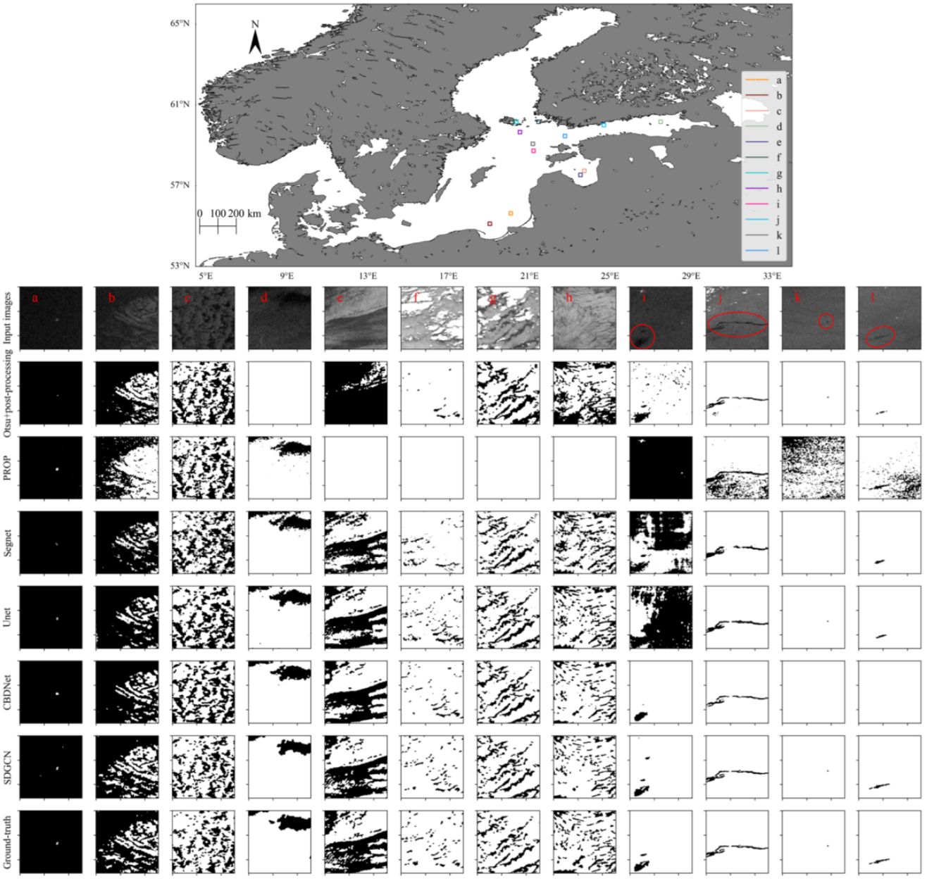
Figure 5 depicts the results of dark spot segmentation in 12 representative SAR images with different brightness levels. The first four images are rather dark in brightness, whereas the middle four images are relatively bright, and the last four images contain the observed oil slicks. As can be seen, the boundaries of the dark spots in images b, d, e, f, h, and i are indistinct, while the borders of dark spots in other images are apparent. On images with obvious dark spot borders, we can see that only the PROP technique shows poor segmentation performance, with no significant difference between the other methods. The reason is that the PROP technique employs just a few artificial features, and its segmentation results are heavily influenced by speckle noise in SAR images. However, on images with fuzzy dark areas, such as images d, e, and i, Otsu+post-processing, PROP, Segnet, and U-Net all perform badly, with the first two models doing much worse than the latter two. Many darker backgrounds were mislabeled as dark spots, and some lighter dark spots were mislabeled as backgrounds as well. Furthermore, due to the influence of speckle noise in SAR images, the boundaries of dark spots obtained by segmentation are also relatively rough. Compared with other methods, CBD-Net and our SDGCN are less influenced by speckle noise and can obtain relatively smooth dark spot boundaries. However, when the area of dark spots is small, such as oil slicks in images k and l, CBD-Net may smooth them out as noise, increasing the missing rate of oil spill patches, but our SDGCN approach can detect this type of dark spot. Overall, our method can more accurately identify the contours of dark spots in SAR images while reducing noise. Compared with the other models, the results of SDGCN were the most similar to the truth labels, and the dark spots with blurred edges were accurately segmented.

5. Discussion

In this section, we analyze and discuss the practicality and limitations of the SGDCN approach using a larger dataset.
The new dataset contains 27 large-scale ENVISAT SAR images, each with at least one oil patch in sites identified by the Baltic Marine Environment Protection Commission (Helsinki Commission-HELCOM), for a total of approximately more than 100 oil patches. It is difficult to say how many of these oil patches there are because some of them have been shattered into small plaques by the waves. Furthermore, the shape, size, and character of these oil patches are different owing to the influence of factors such as water temperature, salinity, current speed, and the volume of oil discharged. Likewise, these datasets contain a plethora of lookalikes of various shapes and sizes. We retrained the SDGCN model using about 4500 images of 256 × 256 pixels, and then used the trained model to segment all the dark spots on these 27 SAR images.
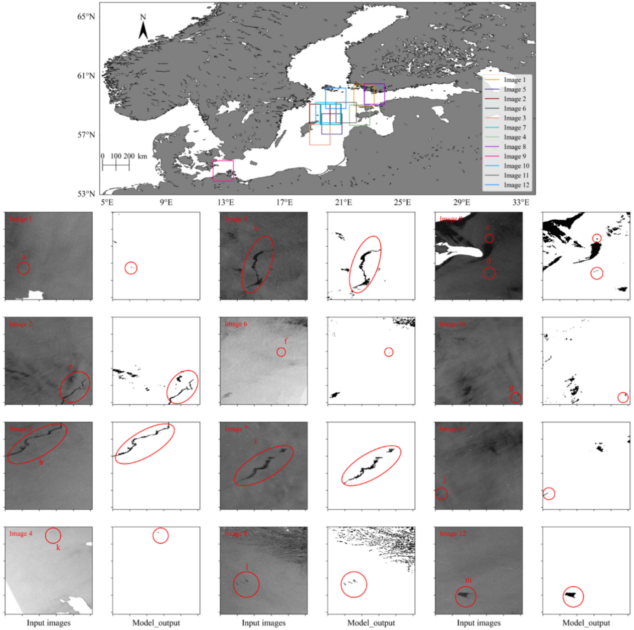
According to our statistics, a total of 103 oil pieces were detected in 27 images. The smallest oil spill patch detected was 0.2 km2, while the largest was 245 km2. We applied the CMOD5 geophysical model function to derive the wind speeds of the sea surface for oil spill analysis and discovered that the wind speed on the sea surface of all the oil patches segmented ranged from 1 to 8 m/s. However, Garcia-Pineda et al. [45] determined that the optimum wind speed range to study the surface of oil slicks in SAR images was 3.5~7.0 m/s. As can be seen, our SDGCN performs well in oily patch segmentation. In Figure 6, we display some representative oil patches detected. Additional oil patches and lookalikes that were segmented are available in the Supplementary Material. From Figure 6, we can see that they vary in terms of size, shape, and brightness, and that almost all of them were formed by illegal discharge from ships. Oil patches a, c, f, g, and k appear as dots with small areas, oil patch m appears as a lump shape, and the remaining oil patches appear as long strips. Furthermore, oil patches a, f, and k have fuzzy edges and are less clearly distinguished from the background, but other oil patches have rather defined boundaries. We can intuitively see that the segmentation results of our SDGCN model basically look the same as the oil patches on the input image.
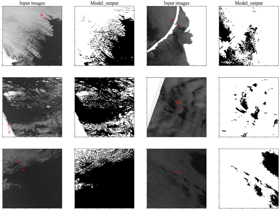
Figure 7 shows the unsegmented oil patches in all the images. It can be seen that only a small proportion of oil patches with weak borders and small areas shattered by waves were missed. They appear to be extremely small and very similar to the surrounding background. Obviously, their oil leakage is minimal. Furthermore, phenomena [46] such as advection, diffusion, evaporation, emulsification, and so on may have significantly altered their properties, causing them to appear similar to the oceanic background in the image. As can be seen, our SDGCN is incapable of segmenting all oily dark spots of this type accurately despite improving dark spot segmentation performance. Further study is needed in the future to enhance the detection performance of dark patches with weak borders and small areas.
Aside from oil slicks, many meteorological or oceanic phenomena, such as upwelling, rain cells, wind shadowing, ocean currents [29], and high chlorophyll-a concentration [47] can also smooth the surface of the sea and produce weak backscatter, which appears as dark spots on SAR images [7]. Typically, these non-oil dark spots account for the vast majority of dark spots [8]. Figure 8 shows several examples of various lookalikes successfully segmented. In addition, Table 5 depicts the characteristics of the atmosphere and ocean surface of these lookalikes, including wind speed, ocean currents, chlorophyll-a concentration, and temperature difference between the atmosphere and ocean. Except for the wind speed, which we derived using the CMOD5 model, other meteorological and marine data were provided by the European Center for Medium-Term Weather Forecast (ECMWF).
In Figure 8, dark spots a, c, and e are the low wind areas where the wind speed was lower than 0.6 m/s. The low wind speed resulted in a smooth sea surface, so these areas appeared as dark spots on the images. Typically, low wind-caused dark spots compose the vast majority of lookalikes on the SAR images. The concentration of chlorophyll-a in the dark spot b area was 17.400 mg/m3, which is relatively high. This dark spot may have been caused by an abnormal chlorophyll-a concentration. The air–sea temperature difference in the dark spot d area was relatively large at 3.655 k. This dark spot may have been caused by an upwelling, which brings the cold water from the lower layer to the upper layer. On radar imaging, the temperature drop is usually followed by a decrease in the roughness of the sea surface, which appears as a dark spot [29]. The dark spot f may have been caused by the sea currents, which can cause biogenic oil to accumulate in some regions and change the roughness of the sea surface, making these areas appear as black spots on SAR images [29]. As far as the various causes and shapes of lookalikes, it can be seen that the segmentation results of the SDGCN model were basically the same as the dark spots on the input image. The segmentation results of the model were nearly satisfactory.
Following the results of the preceding experiments, it is clear that our proposed SDGCN model increases the performance of dark point segmentation. However, it has some limitations. Specifically, it requires some complicated steps to implement, including transforming images to graphs with superpixels as nodes, feature extraction and selection of nodes, and graph node classification, all of which can affect the performance of dark spot segmentation. In the first step, affected by the performance of the superpixel segmentation algorithm, there are a few dark spots with small regions and weak bounds whose contours are difficult to detect, resulting in missing detection. Furthermore, the SDGCN algorithm is time-consuming, especially in superpixel segmentation and feature extraction. As a result, higher performance superpixel segmentation algorithms must be developed in the future to improve the accuracy of contour detection and reduce time consumption. Additionally, we need to find features that are better suited for dark spot segmentation in order to accelerate the feature extraction process. Dark spot detection is only the beginning of oil spill detection. In the future, we plan to conduct follow-up research on oil spill detection, such as dark spot feature extraction and dark spot classification. Moreover, we intend to create a knowledge graph [48,49] to aid in the storage and query of oil spills.

6. Conclusions

In this paper, we propose an efficient dark spot segmentation method that can significantly improve dark spot detection on a single-polarized SAR image. Our method consists of three steps: (1) converting images to graphs with superpixels as nodes; (2) feature extraction and selection of superpixels; and (3) graph node classification. SAR image superpixelation can aid in accurately detecting the contours of blurred dark spots while smoothing out image noise. Following that, the image is transformed into a graph structure with superpixels as nodes and fed into a deep graph neural network for graph node classification, which reduces the computational burden significantly. To improve classification performance, we compute a vector of 137 feature values for each superpixel node and use the SVM-RFE algorithm to select an excellent feature subset of 30 feature values. The proposed feature subset not only accelerates the feature extraction process but also improves the accuracy of the model. Among the selected features, the physical features played a major role, followed by the geometric features and the textural features. The experimental results show that our method outperforms pixel-based segmentation methods and can segment the vast majority of dark spots, except for a few with smaller shapes and brightness levels that are very close to the background. Due to the general characteristics of the SDGCN model, it can be easily extended to address applications such as semantic segmentation of optical remote sensing images [50,51]. In future work, we therefore intend to explore that possibility. Moreover, we will continue the follow-up work on dark spot detection. The dark spots segmented from the image will be used as entities to create a knowledge graph [48] for oil spill detection. Then, we will explore knowledge inference methods to identify oil slicks.

Supplementary Materials

The following supporting information can be downloaded at: https://www.mdpi.com/article/10.3390/rs14215618/s1, Figure S1: The successfully segmented look-alikes; Figure S2: The successfully segmented oil patches. Dark spots in the red area are oil patches; Figure S3: The successfully segmented oil patches. Dark spots in the red area are oil patches.

Author Contributions

Conceptualization, X.L. (Xiaojian Liu); Data curation, X.L. (Xiaojian Liu); Funding acquisition, Y.L. and X.L. (Xinyi Liu); Methodology, X.L. (Xiaojian Liu); Project administration, Y.L. and X.L. (Xinyi Liu); Visualization, X.L. (Xiaojian Liu); Writing—original draft, X.L. (Xiaojian Liu); Writing—review and editing, Y.L., X.L. (Xinyi Liu) and H.Z. All authors have read and agreed to the published version of the manuscript.

Funding

This work was funded by the National Natural Science Foundation of China under grant 41971284 and 42192581; the Fundamental Research Funds for the Central Universities under grant 2042022kf1201; Zhizhuo Research Fund on Spatial-Temporal Artificial Intelligence under grant ZZJJ202210; the Special Fund of Hubei Luojia Laboratory under grant 220100032; The Special Fund of Hubei Luojia Laboratory 220100032.

Institutional Review Board Statement

Not applicable.

Data Availability Statement

All data in this study can be downloaded from the published link.

Acknowledgments

The authors are very grateful to Guohao Li, Roy Uziel and David Mera for code support and the ESA and the Baltic Marine Environment Protection Commission (Helsinki Commission—HELCOM) for data support.

Conflicts of Interest

The authors declare no conflict of interest.

References

  1. Cheng, L.; Li, Y.; Zhang, X.; Xie, M. An Analysis of the Optimal Features for Sentinel-1 Oil Spill Datasets Based on an Improved J–M/K-Means Algorithm. Remote Sens. 2022, 14, 4290. [Google Scholar] [CrossRef]
  2. Rousso, R.; Katz, N.; Sharon, G.; Glizerin, Y.; Kosman, E.; Shuster, A. Automatic Recognition of Oil Spills Using Neural Networks and Classic Image Processing. Water 2022, 14, 1127. [Google Scholar] [CrossRef]
  3. Feng, J.; Chen, H.; Bi, F.; Li, J.; Wei, H. Detection of oil spills in a complex scene of SAR imagery. Sci. China Technol. Sci. 2014, 57, 2204–2209. [Google Scholar] [CrossRef]
  4. Solberg, A.H.S. Remote Sensing of Ocean Oil-Spill Pollution. Proc. IEEE 2012, 100, 2931–2945. [Google Scholar] [CrossRef]
  5. Chen, L.; Ni, J.; Luo, Y.; He, Q.; Lu, X. Sparse SAR Imaging Method for Ground Moving Target via GMTSI-Net. Remote Sens. 2022, 14, 4404. [Google Scholar] [CrossRef]
  6. Li, Y.; Li, J. Oil spill detection from SAR intensity imagery using a marked point process. Remote Sens. Environ. 2010, 114, 1590–1601. [Google Scholar] [CrossRef]
  7. Shu, Y.; Li, J.; Yousif, H.; Gomes, G. Dark-spot detection from SAR intensity imagery with spatial density thresholding for oil-spill monitoring. Remote Sens. Environ. 2010, 114, 2026–2035. [Google Scholar] [CrossRef] [Green Version]
  8. Topouzelis, K.N. Oil Spill Detection by SAR Images: Dark Formation Detection, Feature Extraction and Classification Algorithms. Sensors 2008, 8, 6642–6659. [Google Scholar] [CrossRef] [Green Version]
  9. Chehresa, S.; Amirkhani, A.; Rezairad, G.-A.; Mosavi, M.R. Optimum Features Selection for oil Spill Detection in SAR Image. J. Indian Soc. Remote Sens. 2016, 44, 775–787. [Google Scholar] [CrossRef]
  10. Solberg, A.H.S.; Brekke, C.; Husoy, P.O. Oil Spill Detection in Radarsat and Envisat SAR Images. IEEE Trans. Geosci. Remote Sens. 2007, 45, 746–755. [Google Scholar] [CrossRef]
  11. Topouzelis, K.; Karathanassi, V.; Pavlakis, P.; Rokos, D. Dark formation detection using recurrent neural networks and SAR data. In Proceedings of the Image and Signal Processing for Remote Sensing XII, Stockholm, Sweden, 11–14 September 2006; pp. 324–330. [Google Scholar] [CrossRef]
  12. Taravat, A.; Latini, D.; Del Frate, F. Fully Automatic Dark-Spot Detection From SAR Imagery With the Combination of Nonadaptive Weibull Multiplicative Model and Pulse-Coupled Neural Networks. IEEE Trans. Geosci. Remote Sens. 2014, 52, 2427–2435. [Google Scholar] [CrossRef]
  13. Lang, H.; Zhang, X.; Xi, Y.; Zhang, X.; Li, W. Dark-spot segmentation for oil spill detection based on multifeature fusion classification in single-pol synthetic aperture radar imagery. J. Appl. Remote Sens. 2017, 11, 15006. [Google Scholar] [CrossRef]
  14. Xu, L.; Shafiee, M.J.; Wong, A.; Clausi, D.A. Fully Connected Continuous Conditional Random Field With Stochastic Cliques for Dark-Spot Detection In SAR Imagery. IEEE J. Sel. Top. Appl. Earth Obs. Remote Sens. 2016, 9, 2882–2890. [Google Scholar] [CrossRef]
  15. Guo, H.; Wei, G.; An, J. Dark Spot Detection in SAR Images of Oil Spill Using Segnet. Appl. Sci. 2018, 8, 2670. [Google Scholar] [CrossRef] [Green Version]
  16. Cantorna, D.; Dafonte, C.; Iglesias, A.; Arcay, B. Oil spill segmentation in SAR images using convolutional neural networks. A comparative analysis with clustering and logistic regression algorithms. Appl. Soft Comput. 2019, 84, 105716. [Google Scholar] [CrossRef]
  17. Yekeen, S.T.; Balogun, A.L. Automated Marine Oil Spill Detection Using Deep Learning Instance Segmentation Model. Int. Arch. Photogramm. Remote Sens. Spat. Inf. Sci. 2020, 43, 1271–1276. [Google Scholar] [CrossRef]
  18. Dollár, K.H.G.G.P.; Girshick, R. Mask r-cnn. In Proceedings of the IEEE International Conference on Computer Vision, Venice, Italy, 22–29 October 2017; pp. 2961–2969. [Google Scholar]
  19. Simonyan, K.; Zisserman, A. Very deep convolutional networks for large-scale image recognition. arXiv 2014, arXiv:1409.1556. [Google Scholar]
  20. Zeng, K.; Wang, Y. A Deep Convolutional Neural Network for Oil Spill Detection from Spaceborne SAR Images. Remote Sens. 2020, 12, 1015. [Google Scholar] [CrossRef] [Green Version]
  21. Basit, A.; Siddique, M.A.; Bhatti, M.K.; Sarfraz, M.S. Comparison of CNNs and Vision Transformers-Based Hybrid Models Using Gradient Profile Loss for Classification of Oil Spills in SAR Images. Remote Sens. 2022, 14, 2085. [Google Scholar] [CrossRef]
  22. Zhu, Q.; Zhang, Y.; Li, Z.; Yan, X.; Guan, Q.; Zhong, Y.; Zhang, L.; Li, D. Oil Spill Contextual and Boundary-Supervised Detection Network Based on Marine SAR Images. IEEE Trans. Geosci. Remote Sens. 2022, 60, 5213910. [Google Scholar] [CrossRef]
  23. Uziel, R.; Ronen, M.; Freifeld, O. Bayesian Adaptive Superpixel Segmentation. In Proceedings of the 2019 IEEE/CVF International Conference on Computer Vision (ICCV), Seoul, Korea, 27 October–2 November 2019; pp. 8469–8478. [Google Scholar]
  24. Zhang, J.; Feng, H.; Luo, Q.; Li, Y.; Zhang, Y.; Li, J.; Zeng, Z. Oil Spill Detection with Dual-Polarimetric Sentinel-1 SAR Using Superpixel-Level Image Stretching and Deep Convolutional Neural Network. Remote Sens. 2022, 14, 3900. [Google Scholar] [CrossRef]
  25. Li, Y.; Chen, W.; Huang, X.; Gao, Z.; Li, S.; He, T.; Zhang, Y. MFVNet: Deep Adaptive Fusion Network with Multiple Field-of-Views for Remote Sensing Image Semantic Segmentation. Sci. China Inform. Sci. 2022. [Google Scholar] [CrossRef]
  26. Li, G.; Muller, M.; Thabet, A.; Ghanem, B. DeepGCNs: Can GCNs Go As Deep As CNNs? In Proceedings of the 2019 IEEE/CVF International Conference on Computer Vision (ICCV), Seoul, Korea, 27 October–2 November 2019; pp. 9266–9275. [Google Scholar]
  27. Liu, M.; Gao, H.; Ji, S. Towards Deeper Graph Neural Networks. In Proceedings of the 26th ACM SIGKDD International Conference on Knowledge Discovery & Data Mining, Virtual, 6–10 July 2020; pp. 338–348. [Google Scholar]
  28. European Space Agency. ASAR Product Handbook; ESA: Paris, France, 2007; pp. 94–97. [Google Scholar]
  29. Najoui, Z.; Riazanoff, S.; Deffontaines, B.; Xavier, J.-P. A Statistical Approach to Preprocess and Enhance C-Band SAR Images in Order to Detect Automatically Marine Oil Slicks. IEEE Trans. Geosci. Remote Sens. 2018, 56, 2554–2564. [Google Scholar] [CrossRef]
  30. Konik, M.; Bradtke, K. Object-oriented approach to oil spill detection using ENVISAT ASAR images. ISPRS J. Photogramm. Remote Sens. 2016, 118, 37–52. [Google Scholar] [CrossRef]
  31. Misra, A.; Balaji, R. Simple Approaches to Oil Spill Detection Using Sentinel Application Platform (SNAP)-Ocean Application Tools and Texture Analysis: A Comparative Study. J. Indian Soc. Remote Sens. 2017, 45, 1065–1075. [Google Scholar] [CrossRef]
  32. Genovez, P.; Ebecken, N.; Freitas, C.; Bentz, C.; Freitas, R. Intelligent hybrid system for dark spot detection using SAR data. Expert Syst. Appl. 2017, 81, 384–397. [Google Scholar] [CrossRef]
  33. Habart, D.; Borovec, J.; Švihlík, J.; Kybic, J. Supervised and unsupervised segmentation using superpixels, model estimation, and graph cut. J. Electron. Imaging 2017, 26, 061610. [Google Scholar] [CrossRef]
  34. Giraud, R.; Ta, V.-T.; Papadakis, N. Robust superpixels using color and contour features along linear path. Comput. Vis. Image Underst. 2018, 170, 1–13. [Google Scholar] [CrossRef] [Green Version]
  35. Solberg, S.; Brekke, C.; Husoy, O. Algorithms for Oil Spill Detection in Radarsat and ENVISAT SAR Images. In Proceedings of the IGARSS 2004, 2004 IEEE International Geoscience and Remote Sensing Symposium, Anchorage, AK, USA, 20–24 September 2007; pp. 4909–4912. [Google Scholar]
  36. Vyas, K.; Shah, P.; Patel, U.; Zaveri, T.; Kumar, R. Oil Spill Detection from SAR Image Data for Remote Monitoring of Marine Pollution Using Light Weight ImageJ Implementation. In Proceedings of the 2015 5th Nirma University International Conference on Engineering (NUiCONE), Ahmedabad, India, 26–28 November 2015; pp. 1–6. [Google Scholar] [CrossRef]
  37. Mera, D.; Bolon-Canedo, V.; Cotos, J.; Alonso-Betanzos, A. On the use of feature selection to improve the detection of sea oil spills in SAR images. Comput. Geosci. 2017, 100, 166–178. [Google Scholar] [CrossRef]
  38. Rong, Y.; Huang, W.; Xu, T.; Huang, J. DropEdge: Towards Deep Graph Convolutional Networks on Node Classification. In Proceedings of the International Conference on Learning Representations (ICLR), Virtual, 26 April–1 May 2020. [Google Scholar]
  39. Kipf, T.N.; Welling, M. Semi-supervised classification with graph convolutional networks. In Proceedings of the International Conference on Learning Representations (ICLR), Toulon, France, 24–26 April 2017. [Google Scholar]
  40. Li, G.; Xiong, C.; Thabet, A.; Ghanem, B. Deepergcn: All you need to train deeper gcns. arXiv 2020, arXiv:2006.07739. [Google Scholar]
  41. Zhang, M.; Chen, Y. Link prediction based on graph neural networks. In Advances in Neural Information Processing Systems; Curran Associates Inc.: Montréal, QC, Canada, 2018; pp. 5171–5181. [Google Scholar]
  42. Lee, J.; Lee, I.; Kang, J.J.A. Self-Attention Graph Pooling. In Proceedings of the 36th International Conference on Machine Learning, Long Beach, CA, USA, 9–15 June 2019. [Google Scholar]
  43. Javan, F.D.; Samadzadegan, F.; Gholamshahi, M.; Mahini, F.A. A Modified YOLOv4 Deep Learning Network for Vision-Based UAV Recognition. Drones 2022, 6, 160. [Google Scholar] [CrossRef]
  44. Ronneberger, O.; Fischer, P.; Brox, T. U-Net: Convolutional Networks for Biomedical Image Segmentation. In Proceedings of the 18th International Conference, Medical Image Computing and Computer-Assisted Intervention, MICCAI 2015, Munich, Germany, 5–9 October 2015; pp. 234–241. [Google Scholar]
  45. Garcia-Pineda, O.; Zimmer, B.; Howard, M.; Pichel, W.G.; Li, X.; MacDonald, I.R. Using SAR images to delineate ocean oil slicks with a texture-classifying neural network algorithm (TCNNA). Can. J. Remote Sens. 2009, 35, 411–421. [Google Scholar] [CrossRef]
  46. Berry, A.; Dabrowski, T.; Lyons, K. The oil spill model OILTRANS and its application to the Celtic Sea. Mar. Pollut. Bull. 2012, 64, 2489–2501. [Google Scholar] [CrossRef] [PubMed] [Green Version]
  47. Alpers, W.; Holt, B.; Zeng, K. Oil spill detection by imaging radars: Challenges and pitfalls. Remote Sens. Environ. 2017, 201, 133–147. [Google Scholar] [CrossRef]
  48. Hao, X.; Ji, Z.; Li, X.; Yin, L.; Liu, L.; Sun, M.; Liu, Q.; Yang, R. Construction and Application of a Knowledge Graph. Remote Sens. 2021, 13, 2511. [Google Scholar] [CrossRef]
  49. Li, Y.; Kong, D.; Zhang, Y.; Tan, Y.; Chen, L. Robust deep alignment network with remote sensing knowledge graph for zero-shot and generalized zero-shot remote sensing image scene classification. ISPRS J. Photogramm. Remote Sens. 2021, 179, 145–158. [Google Scholar] [CrossRef]
  50. Pu, W.; Wang, Z.; Liu, D.; Zhang, Q. Optical Remote Sensing Image Cloud Detection with Self-Attention and Spatial Pyramid Pooling Fusion. Remote Sens. 2022, 14, 4312. [Google Scholar] [CrossRef]
  51. Liu, B.; Hu, J.; Bi, X.; Li, W.; Gao, X. PGNet: Positioning Guidance Network for Semantic Segmentation of Very-High-Resolution Remote Sensing Images. Remote Sens. 2022, 14, 4219. [Google Scholar] [CrossRef]
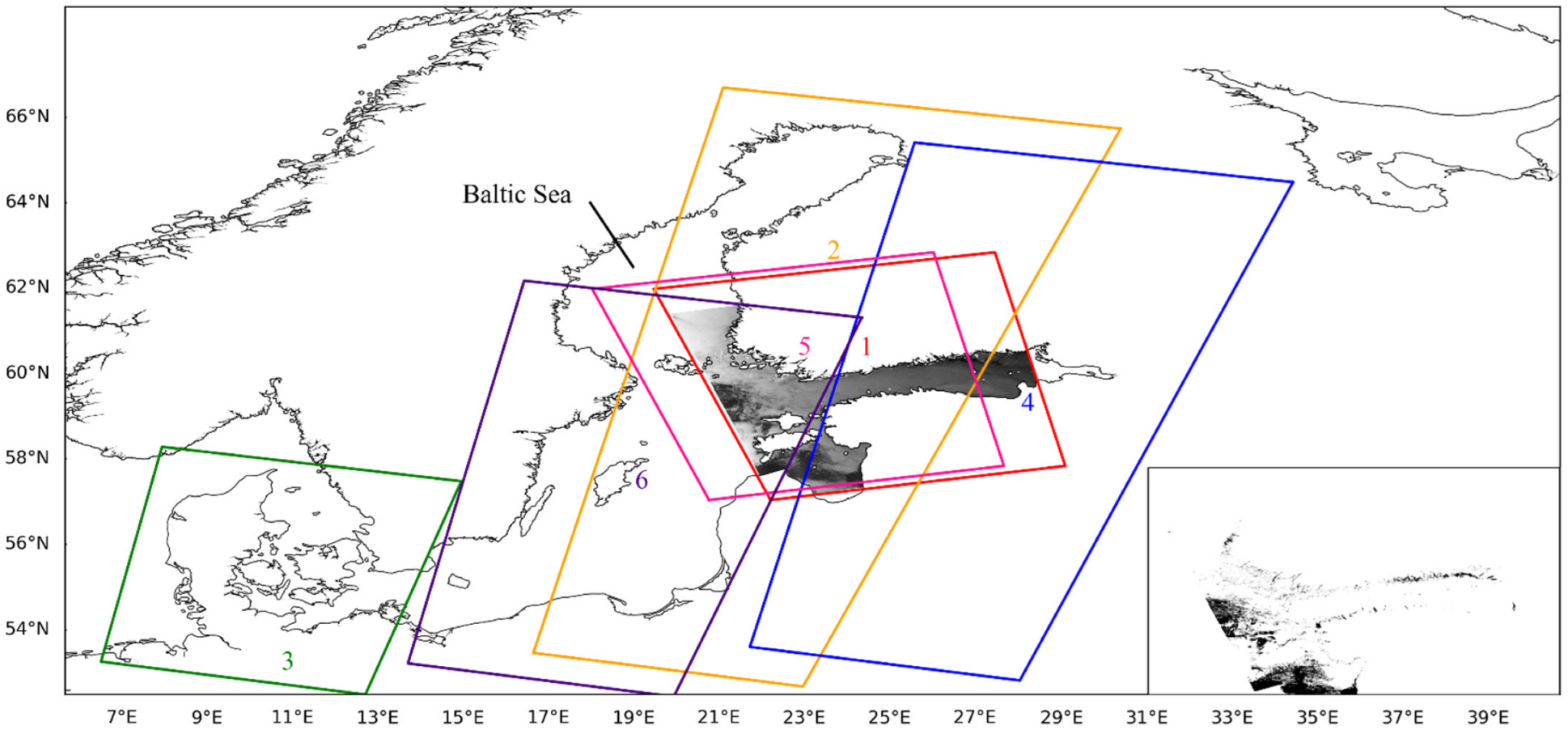
Figure 1. Overview of the research area. Numbers 1 through 6 show the coverage of the images used; and the artificially marked dark spots in image 1 are shown in the lower right corner.
Remotesensing 14 05618 g001
Figure 2. Workflow of the proposed dark spot segmentation method. (a) depicts the process of transforming the image into a graph structure, (b) depicts feature extraction and selection, and (c) depicts final graph node classification.
Remotesensing 14 05618 g002
Figure 3. Conversion of the image to non-Euclidean structure data. (a) depicts superpixel segmentation in a SAR image, (b) describes the transformation of SAR images into graph structures with superpixels as nodes, and (c) depicts the removal of land nodes and the edges that connect to them.
Remotesensing 14 05618 g003
Figure 4. F1 score for dark spot segmentation using various feature-value combinations.
Remotesensing 14 05618 g004
Figure 5. A few examples of qualitative comparison results. a~l are the various SAR images (256 × 256 pixels) that were used. The top panel shows the locations of images a~l, respectively. Images a~h contain lookalikes of varying shapes and sizes, with images a~d being darker and images e~h being brighter. The red regions in the SAR images a through h depict oil slicks of varied shapes and sizes.
Remotesensing 14 05618 g005
Figure 6. The successful segmentation of oil patches of various shapes and sizes in different images. The top panel shows the locations of all images. In other panels, the dark spots in the red circles are the oil patches and a~m are their numbers.
Remotesensing 14 05618 g006
Figure 7. Oil patches that were missed. The top panel shows the locations of all images. The red circles in the input images indicate the oil patches that were not successfully segmented.
Remotesensing 14 05618 g007
Figure 8. The segmentation results of various lookalikes; the a~f arrows point to the dark spots.
Remotesensing 14 05618 g008
Table 1. Geometric, texture, and physical features computed for superpixels in this study.
NoFeatureCodeCategoryNoFeatureCodeCategory
1AreaAGeometrical25Var_area_superpixelVasTextura
2PerimeterPGeometrical26Mean HaralickHTextura
3Perimeter to area ratioP/AGeometrical27Object meanOmPhysical
4Area to perimeter ratioA/PGeometrical28Object standard deviationOsdPhysical
5ElongationEGeometrical29Background meanBmPhysical
6Major axis to perimeter ratioMaxx/PGeometrical30Background standard deviationBsdPhysical
7Complexity1Cp1Geometrical31Mean of the contrast ratioCrmPhysical
8Complexity2Cp2Geometrical32Standard deviation of the contrast ratioCrsdPhysical
9CircularityCGeometrical33Object power to meanOpmPhysical
10SpreadingSGeometrical34Background power to meanBpmPhysical
11Superpixel widthSwGeometrical35Ratio of the power to mean ratiosOpm/BpmPhysical
12CurvatureCuGeometrical36Max contrastCmaxPhysical
13Hu momentsHuGeometrical37Mean contrastCmPhysical
14Fluser and Suk momentsFsGeometrical38RISDIRISDIPhysical
15ThicknessTGeometrical39RISDORISDOPhysical
16Shape connectivityShcGeometrical40IORIORPhysical
17Form factorFfGeometrical41Gradient meanGmPhysical
18Length to width ratioL/WGeometrical42Gradient standard deviationGsdPhysical
19Shape indexSiGeometrical43Max. gradientGmaxPhysical
20NarrownessNGeometrical44Object border gradientObgPhysical
21Rectangular saturationRsGeometrical45Surrounding Power-to-mean ratioSpmPhysical
22Marking ratioMrGeometrical46RIIARIIAPhysical
23SoliditySdGeometrical47Elliptic Fourier DescriptorsEFDGeometrical
24Mean of the interior angles based on bounding polygonsIABPmGeometrical48Standard deviation of the interior angles based on bounding polygonsIABPsdGeometrical
Table 2. A subset of features obtained for dark spot segmentation using the SVM-RFE algorithm.
RankCodeCategoryRankCodeCategoryRankCodeCategory
1RIIAPhysical11Fs4Geometrical21BsdPhysical
2CmPhysical12Cp1Geometrical22IORPhysical
3ObgPhysical13VasTextural23BpmPhysical
4GmPhysical14A/PGeometrical24BmPhysical
5RISDOPhysical15Fs3Geometrical25Cp2Geometrical
6AGeometrical16RISDIPhysical26L/WGeometrical
7PGeometrical17SpmPhysical27EGeometrical
8CGeometrical18RsGeometrical28SiGeometrical
9OmPhysical19SdGeometrical29P/AGeometrical
10OsdPhysical20MrGeometrical30TGeometrical
Table 3. Comparison of the top 30 feature values with all feature values.
ModelPd (100%)Pf (100%)F1 Sore (100%)Pm (100%)
SDGCN with the top 30 feature values96.985.6895.637.18
SDGCN with all feature values95.746.6894.528.73
Table 4. Comparison between our proposed SDGCN algorithm and different dark spot segmentation methods.
MethodPd (100%)Pf (100%)F1 Score (100%)Pm (100%)
Otsu+post-processing [9]71.7412.7878.7326.35
PROP [13]90.3652.7162.0910.36
SegNet [15]83.008.8887.0213.03
UNet [37]83.206.6987.969.68
CBD-Net [17]91.9910.7090.6225.30
Our SDGCN96.985.6895.637.18
Table 5. Ocean and atmospheric characteristics of the lookalikes in Figure 8.
Dark SpotMean Wind (m/s)Mean Sea
Water Velocity (m/s)
Mean Convective Rain Rate
(kg·m−2·s−1)
The Temperature
Difference between the
Atmosphere and the Ocean (K)
Mean Chlorophyll-a
Concentration (mg/m3)
a0.1950.08800.6352.128
b4.0090.0400−0.70417.400
c0.2890.05800.2012.459
d4.7500.08303.6550
e0.5530.07800.1442.635
f4.0120.2060−0.6892.673
Publisher’s Note: MDPI stays neutral with regard to jurisdictional claims in published maps and institutional affiliations.