Abstract
Phytoplankton in the northwest Pacific plays an important role in absorbing atmospheric CO2 and promoting the ocean carbon cycle. However, our knowledge on the long-term interannual variabilities of the phytoplankton biomass in this region is quite limited. In this study, based on the Chlorophyll-a concentration (Chl-a) time series observed from ocean color satellites of Sea-viewing Wide Field-of-view Sensor (SeaWiFS) and Moderate Resolution Imaging Spectroradiometer (MODIS) in the period of 1997–2020, we investigated the variabilities of Chl-a on both seasonal and interannual scales, as well as the long-term trends. The phytoplankton Chl-a showed large spatial dynamics with a general decreasing pattern poleward. The seasonal phytoplankton blooms dominated the seasonal characteristics of Chl-a, with spring and fall blooms identified in subpolar waters and single spring blooms in subtropical seas. On interannual scales, we found a Chl-a increasing belt in the subpolar oceans from the marginal sea toward the northeast open ocean waters, with positive trends (~0.02 mg m−3 yr−1, on average) in Chl-a at significant levels (p < 0.05). In the subtropical gyre, Chl-a showed slight but significant negative trends (i.e., <−0.0006 mg m−3 yr−1, at p < 0.05). The negative Chl-a trends in the subtropical waters tended to be driven by the surface warming, which could inhibit nutrient supplies from the subsurface and thus limit phytoplankton growth. For the subpolar waters, although the surface warming also prevailed over the study period, the in situ surface nitrate reservoir somehow showed significant increases in the targeted spots, indicating potential external nitrate supplies into the surface layer. We did not find significant connections between the Chl-a interannual variabilities and the climate indices in the study area. Environmental data with finer spatial and temporal resolutions will further constrain the findings.
1. Introduction
The relationship between ocean ecosystems and global climate change is currently attracting much attention [1,2]. As the base of the marine food web, phytoplankton plays a fundamental role in the biogeochemical cycling of elements by converting inorganic elements into organic components. On one hand, the primary production of phytoplankton communities supports organisms at higher trophic levels and is essential to promoting fishery productions [3,4]. On the other hand, phytoplankton in the ocean contributes to roughly half of the fixed carbon on the planet by absorbing atmospheric CO2, significantly alleviating global warming [5,6]. However, future projections show that the phytoplankton community structure is getting increasingly unstable, and the primary production is decreasing in response to climate change [7,8].
The quantity and quality of phytoplankton are affected by various environmental forcings, such as light conditions, seawater temperature, marine heatwaves, nutrients, zooplankton grazing pressure, and phytoplankton species composition [9,10,11,12,13,14]. Phytoplankton blooms occur when the phytoplankton biomass shows a sharp increase within a short period. A typical example is the dual seasonal blooms in spring and autumn in mid-latitude seas [15,16]. Different from harmful algal blooms such as red tides, seasonal phytoplankton blooms are driven by the adapted biological phenology, in response to the seasonal changes of the ocean environment [17]. Chlorophyll-a concentration (Chl-a, mg m−3) is an important parameter indicating the phytoplankton biomass and abundance in the ocean ecosystem [18,19]. The total phytoplankton biomass within the euphotic layer is highly correlated with surface Chl-a in a nonlinear fashion [20,21]. The accumulation of the ocean color satellite remote sensing of sea surface Chl-a in the past decades provides a reliable data source for studying the phytoplankton dynamics on long time scales [22,23,24,25]. Ocean color remote sensing is characterized by synoptic observations in the ocean surface layer. Phenomena such as deep Chl-a maxima cannot be detected from space in most cases, except in the presence of, e.g., internal tides [26]. The satellite retrievals of Chl-a are subject to multiple error sources (e.g., clouds, sun glint, large solar angles, stray light), with a general uncertainty of 5–35% [27,28], serving as a reliable data reservoir for studies on large spatial and long time scales.
The northwest Pacific supports a strong carbon sink and high primary production and plays an important role in global carbon cycling [29,30,31]. The warm Kuroshio current and cold Oyashio current are the two largest ocean currents dominating the ocean circulation in this region (Figure 1). The warm currents are characterized by low nutrients (i.e., oligotrophic waters), and the cold currents are nutrient-enriched, together modulating the spatial distributions of nutrients and the physical-biogeochemical dynamics in the northwest Pacific [32]. A few studies attempted to investigate the dynamics of phytoplankton biomass and primary production in the East/Japan Sea of the northwest Pacific. Based on satellite observations of sea surface Chl-a from the Sea-viewing Wide Field-of-view Sensor (SeaWiFS) from 1998 to 2002, Yamada et al. [22] characterized the timing of spring and fall blooms in the East Sea and found that the start of the spring bloom was correlated with surface wind speed, but this was not the case for the fall bloom. Using a Gaussian fitting curve of the SeaWiFS Chl-a dynamics between 1998 and 2003, Yamada & Ishizaka [33] estimated that the spring bloom started and peaked relatively earlier in March, with a shorter duration in the mid-1980s. Lee et al. [34] reviewed the past progress on the spatial and temporal variability of the pelagic ecosystem in the East Sea and found that the long-term changes of phytoplankton biomass and the physical-biological environments were associated with climate variability in this region. Similarly, Joo et al. [35] reported a decreasing trend (13% per decade) of the annual primary production from the Moderate Resolution Imaging Spectroradiometer (MODIS) in the East Sea between 2003 and 2012, which was attributed to the shallower mixed layers caused by the increased seawater temperature and the Pacific Decadal Oscillation (PDO) [36]. In contrast, using a MODIS satellite data record of Chl-a between 2003 and 2020, Park et al. [37,38] recently found that the Chl-a in the East Sea tended to increase over the years, with some spatial divergence. Overall, in addition to these controversial findings in the East Sea, a big knowledge gap exists in the broad northwest Pacific about the phytoplankton Chl-a dynamics in recent decades, for which the satellite views of the seasonal and interannual variability of the phytoplankton Chl-a in this region from SeaWiFS and MODIS over the past 23 years (1997–2020) neatly fit in the scope.
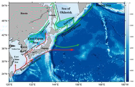
Figure 1.
Bathymetric map (unit: m) of the northwest Pacific, based on the ETOPO2 bathymetry, with red lines representing warm currents and green lines representing cold currents.
Under global warming and climate change, studies show that the global ocean has been more stratified over the last half century, inhibiting the transport of heat, carbon, and other constituents from the surface into the ocean interior [39,40,41,42]. In turn, ocean stratification also leads to a decrease in ocean mixing, which could amplify warming in the upper ocean layer and inhibit vertical nutrient supply from the deep waters to the upper waters as well [42]. Investigations of different environmental factors that modulated the seasonal and interannual dynamics of Chl-a were attempted in some regional seas. For example, Kilpatrick et al. [43] found that the Chl-a dynamics in the Southern California Bight were mainly driven by the local upwelling effect, with a strong negative correlation with sea surface temperature (SST, °C). Similarly, Yu et al. [44] found that the monsoon winds and SST most determined the spatial and temporal variability of Chl-a in the South China Sea. Siswanto et al. [45] found strong correlations between Chl-a and climate indices in the Indonesian maritime continent. However, little was known about the driving factors of the Chl-a dynamics in the northwest Pacific. With global warming, the decrease in nutrients in the upper ocean layer has resulted in a global decline in phytoplankton primary production and biodiversity [32,40,46]. Recently, anthropogenic emissions of nitrate by fossil fuel combustion and modern agriculture have drawn public attention. Kim et al. [47,48] investigated the nitrate dynamics in the Northwest Pacific in recent decades and found that, despite the weakened vertical mixing under global warming, the abundance of nitrogen relative to phosphorus has increased significantly since 1980 due to the air deposition of anthropogenic nitrogen. The additional nitrogen input should alleviate nitrate limitation and promote phytoplankton growth in the northwest Pacific. However, our current understanding on the phytoplankton dynamics in this region is quite limited. To promote our knowledge on the dynamics of phytoplankton biomass and its driving factors in the northwest Pacific, therefore, the objectives of this study include: (1) investigate the seasonal and interannual variabilities of Chl-a from SeaWiFS and MODIS in the past 23 years (1997–2020); (2) characterize the dominant driving factors of the identified interannual changing patterns in Chl-a; and (3) understand the driving mechanisms of different environmental and climate forcing effects on the dynamics of phytoplankton biomass in the northwest Pacific.
2. Data and Methods
2.1. Satellite Data
Standard daily Level-3 Chl-a data products (version R2018.0) in the period of 1997–2020 were downloaded from the NASA Goddard Space Flight Center (GSFC) (http://oceancolor.gsfc.nasa.gov/, accessed on 21 March 2021). Specifically, Chl-a data collected between September 1997 and December 2002 were obtained from SeaWiFS, and Chl-a data collected between January 2003 and December 2020 were obtained from MODIS on the Aqua satellite. The spatial resolutions of the SeaWiFS and MODIS Chl-a were 9 km and 4 km. The comparison of the Chl-a data time series between SeaWiFS and MODIS in their overlapped orbiting period (2002–2010) showed good agreement with each other (Figure 2), with a mean difference of 0.0077 mg m−3, possibly introduced by their differences in spectral designs, observing geometries, and local overpass times. Correspondingly, the data records of Photosynthetically Available Radiation (PAR, Einstein m−2 d−1) from SeaWiFS and MODIS and those of SST from MODIS, at the same spatial and temporal resolution as that of Chl-a, were also accessed from the NASA GSFC. In addition, Level-3 sea surface wind vectors in the U (west-east) and V (south-north) directions were downloaded from the Remote Sensing Systems (https://www.remss.com/measurements/ccmp/, accessed on 4 July 2021), and these wind data were obtained from the Cross-Calibrated Multi-Platform (CCMP, V2.0) at a spatial resolution of 0.25 degrees. The scalar dataset of the sea surface wind speed (SSW, m s−1) was derived from these U and V wind vectors.
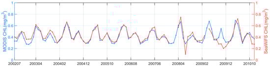
Figure 2.
Time series of the monthly Chl-a in the northwest Pacific, derived from both MODIS and SeaWiFS in their overlapped observation period between July 2002 and November 2010.
2.2. Other Ancillary Data
Due to the lack of sea surface nitrate (SSN, μmol/kg) data products from satellite remote sensing, we used the field nitrate observations as an ancillary dataset in our data analyses. In the northwest Pacific, the World Ocean Database (WOD, version 2018) has accumulated extensive field nitrate observations from various observing platforms (e.g., cruise vessels, buoys, Biogeochemical-Argo floats) in recent decades (i.e., since 1980s). These nitrate data were collected by many different research groups around the world. Tremendous coordinating efforts were made to incorporate data from institutions, agencies, individual researchers, and data initiatives into a single database following a standard data quality control and formatting procedure [49], which provides a precious data reservoir for oceanographic, climatic, and environmental research. We downloaded the WOD nitrate dataset from the NOAA National Centers for Environmental Information (NCEI, https://www.ncei.noaa.gov/products/world-ocean-database, accessed on 23 May 2020). Additionally, the Japan Meteorological Agency (JMA) also maintained the amounts of nitrate data collected from research vessels around the Japan Island in the East Sea or the adjacent open ocean waters of the northwest Pacific. We obtained the JMA nitrate dataset from https://www.jma.go.jp/jma/indexe.html (accessed on 23 July 2020). It should be noted that all these nitrate observations—either from WOD or JMA—are profiling data collected at different water depths. We calculated the SSN within the mixed layer depth using a density threshold of 0.03 kg/m3 [50,51]. In addition, the World Ocean Atlas (WOA) SSN monthly climatologies were downloaded from the NOAA NCEI (https://www.ncei.noaa.gov/products/world-ocean-atlas, accessed on 12 November 2019).
Climate indices data series in the period of 1997–2020 were also selected as ancillary data to help interpret the interannual Chl-a dynamics observed from ocean color. The climate indices used in this study included the multivariate ENSO index (MEI, v2) from the NOAA Physical Sciences Laboratory (PSL, https://psl.noaa.gov/enso/mei/, accessed on 19 September 2022), the Arctic Ocean oscillation index (AOI) from the NOAA Climate Prediction Center (https://www.cpc.ncep.noaa.gov/products/precip/CWlink/daily_ao_index/ao_index.html, accessed on 19 September 2022), and the Pacific Decadal Oscillation (PDO) from NOAA NCEI (https://www.ncei.noaa.gov/access/monitoring/pdo/, accessed on 19 September 2022).
2.3. Methods
Due to cloud, straylight, and sun glint contaminations, large sun zenith angles, etc., daily Chl-a images from ocean color typically have lots of data gaps [52,53]. To increase the spatial coverage of valid Chl-a, we generated the weekly and monthly Chl-a composite images from the daily products of Chl-a for SeaWiFS (1997–2002) and MODIS (2003–2020). The monthly Chl-a images on climatological scales were derived by averaging the monthly Chl-a composites from each year in the period of 1997–2020. For the inconsistency of the spatial resolution between SeaWiFS and MODIS, we linearly interpolated each of the SeaWiFS daily images to a spatial resolution of 4 km, and we declare that this processing had little effect on the data quality of the Chl-a images (e.g., spatial coverage, data ranges which could be slightly reduced) and the results presented in this study. Spatially, the northwest Pacific was divided into two sections along the eastward extension of the Kuroshio around the latitude of 36°N. On seasonal scales, we averaged the monthly Chl-a images for these two sections (i.e., poleward and equatorward of the 36°N) to examine the seasonal differences of Chl-a in the subpolar and subtropical waters. On interannual scales, the anomalies of the monthly Chl-a in 1997–2020 were derived by subtracting the monthly Chl-a climatology from the monthly Chl-a images. As such, we derived the data series of the Chl-a monthly anomaly images in the northwest Pacific between 1997 and 2020. Based on the data series of Chl-a anomalies at each pixel, we conducted a regression analysis to detect the trend in Chl-a in the study period. A t-test was involved in each of the regression analyses, and only trends that passed the confidence tests (at a confidence level of p < 0.05) were shown. Following this processing procedure, we calculated the Chl-a trends on pixel levels (4 km × 4 km) for the broad northwest Pacific.
Phytoplankton growth is mostly influenced by water temperature, solar light conditions, nutrients, and the physical ocean environment. To investigate the potential driving factors and mechanisms of the interannual variabilities of Chl-a in the northwest Pacific, therefore, following the same data processing scheme described above, we also calculated the interannual trends of SST, PAR, and SSW on pixel levels in the northwest Pacific based on the monthly anomalies of each. Specifically, due to the scarcity and coarse spatial and temporal coverage of the field SSN data, we gridded the SSN data on monthly scales at a spatial resolution of 2° × 2° in longitude and latitude following the published studies [47]. A longer data series between 1980 and 2020 was generated for SSN to compensate for the strongly uneven data distributions in terms of data quantity over time. We clarify that, to ensure the sufficiency of the SSN data series for interannual analyses, particularly for the trend detection, a few criteria were set: the data series should cover at least 10 years of data, with the number of monthly means being ≥20 and the data collections being available after the year of 2010. Finally, for the targeted areas in the northwest Pacific, where Chl-a showed significant increasing or decreasing trends, we calculated the correlation coefficients (R) between the Chl-a anomalies data series and the anomalies of SST, PAR, SSW, and SSN, as well as the climate indices (i.e., MEI, AOI, PDO). These statistical measures were used to interpret the potential driving factors and mechanisms of the interannual variabilities and trends in Chl-a.
3. Results
3.1. Seasonal Dynamics
The monthly averaged satellite Chl-a images in the period of 1997–2020 clearly presented the seasonal variability of the phytoplankton biomass in the northwest Pacific, with spatial divergence (Figure 3). Specifically, in the subpolar waters, Chl-a was typically ≥0.5 mg m−3 over the year, with a seasonal variation amplitude of ≥1 mg m−3. Particularly, in the eutrophic marginal seas (e.g., East Sea, China Seas), the seasonal Chl-a was on levels of 1–10 mg m−3, with some spatial difference decreasing from the inshore area towards the offshore area, consistent with the spatial patterns of Chl-a in the published studies [23,37]. In the subtropical gyre, the water was oligotrophic, and Chl-a kept at low levels, with values of ≤~0.2 mg m−3, year-round. It is noted that there was a transition band between the subpolar high Chl-a waters and the subtropical low Chl-a waters. The geo-location of these transition bands had some seasonal migration dynamics, which extended equatorward in fall and winter and stepped poleward in spring and summer. This seasonal migration of the Chl-a transition bands was most likely driven by the seasonal eddy variability in the Kuroshio Extension, where the eddy kinetic energy reached the maximum in the summer and the minimum in the winter [54].
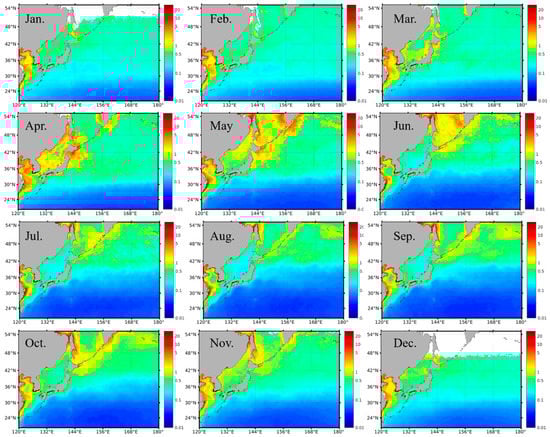
Figure 3.
Spatial distribution of the monthly Chl-a climatology from ocean color in the northwest Pacific, averaged from SeaWiFS and MODIS in the period of 1997–2020. The data gaps (i.e., white pixels) at high latitudes in December and January were mainly caused by the failure of the Chl-a retrieval algorithms at large solar zenith angles (i.e., >60°).
In the subpolar waters, where Chl-a had relatively high values over an annual cycle (Figure 3), the Chl-a showed distinct seasonal dynamics, with peaks in both the spring and fall. Specifically, in spring, with favored light and nutrient conditions, the phytoplankton started to bloom, and the Chl-a reached the annual maxima (>1 mg m−3; in some cases, >5 mg m−3). The magnitude of the spring blooms was around 1 mg m−3. With ocean stratification and nutrient limitation, the Chl-a turned out to be relatively low in the summer. The other algal bloom appeared in the fall. However, the magnitude of the fall blooms in the subpolar waters was around 0.4 mg m−3, much smaller than that of the spring bloom. With the cooling of the surface seawater and the reduction in light penetration in wintertime, the Chl-a reached the seasonal minima. With the increase in latitude, the onset and termination of the seasonal blooms seem to have a delay of one month. For example, in terms of the spring blooms, the phytoplankton within the latitude of 36°–42°N started to bloom in March and vanished in May; yet, the phytoplankton blooms above 42°N initiated in April and ended in June (Figure 3).
In the subtropical oligotrophic waters, the Chl-a was much lower than that in the subpolar regions. Corresponding to the migration of the transition bands of Chl-a in the Kuroshio Extension, the spatial extension of the low Chl-a waters in the subtropical region also showed some seasonal dynamics. Specifically, the bulk of these low Chl-a waters started to expand in the spring, reached spatial maximum in the summer, and then shrank in the fall and winter. From the perspective of seasonal blooms, different from the dual-bloom signals in the subpolar regions, only spring blooms occurred in the subtropical waters. Meanwhile, the magnitude of the spring blooms in the subtropical waters was also significantly smaller than that in the subpolar regions.
To further quantify the seasonal dynamics of the phytoplankton Chl-a in the northwest Pacific, the spatial averages of the Chl-a distributed northward and southward of 36°N, respectively, were extracted to generally represent the Chl-a dynamics in the subpolar and subtropical waters (Figure 4a). Figure 4b shows the derived Chl-a data time series in both sections. As described above, in the subpolar oceans (red curve in Figure 4b), the phytoplankton Chl-a had two peaks in the spring and fall in response to the spring and fall phytoplankton blooms. The spring blooms were much stronger than the fall blooms, which dominated the phytoplankton growth on an annual cycle. In general, the phytoplankton Chl-a had an annual baseline of ~0.5 mg m−3, and it peaked with a Chl-a maximum of ~1.2 mg m−3 and 0.8 mg m−3 in the spring and fall, respectively. In contrast, the phytoplankton Chl-a in the oligotrophic subtropical waters showed much weaker seasonal dynamics (blue curve in Figure 4b), with a seasonal magnitude of ~0.2 mg m−3 in Chl-a, and the baseline of the annual phytoplankton Chl-a was around 0.1 mg m−3. Clearly, different from the dual-peaks of Chl-a in the subpolar waters, the phytoplankton Chl-a only peaked in the spring, suggesting that only spring blooms occurred in the subtropical waters. The Chl-a maxima of the spring phytoplankton blooms were in the order of 0.3 mg m−3, much weaker than those of the spring blooms (i.e., Chl-a maxima of ~1.2 mg m−3) in high-latitude waters.
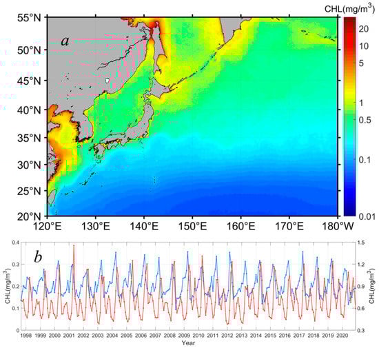
Figure 4.
Spatial distribution of the yearly Chl-a, on average, in 1997–2020 (a), and Chl-a interannual data time series (b) in the subpolar (i.e., poleward of the Kuroshio extension along 36°N, red curve) and subtropical (i.e., equatorward of the Kuroshio extension along 36°N, blue curve) waters of the northwest Pacific (Kuroshio extension southward and northward).
3.2. Interannual Variability and Trends
Figure 4b also shows the interannual variabilities of Chl-a in the northwest Pacific in the period of 1997–2020. In general, the phytoplankton biomass varied from year to year, with differences identified in terms of the amplitude of seasonal blooms, and the maxima and minima of Chl-a in each year. Specifically, in the subpolar waters (i.e., northward of 36°N), the baseline of the phytoplankton Chl-a was 0.46–0.48 mg m−3 in most years of the study period, but it kept a relatively low value of ~0.39 mg m−3 in 2003, 2012, and 2013. The spring bloom peaks showed a clear increase between 1997 and 2002 and kept at levels of 1.2 mg m−3 in the following 18 years, with some interannual variabilities. For example, the spring blooms in 2007, 2008, and 2013 were significantly weaker than those in other years, with Chl-a maxima of 1.0 mg m−3, 0.99 mg m−3, and 0. 91 mg m−3, respectively. Correspondingly, the magnitudes of the spring blooms also varied accordingly in the period of 1997–2020. The mean magnitude of the spring blooms was around 0.8 mg m−3, with a maximum of 1.01 mg m−3 (i.e., Chl-a ranged from 0.44 to 1.45 mg m−3) and a minimum of 0.52 mg m−3 (i.e., Chl-a ranged from 0.39 to 0.91 mg m−3) shown in 2002 and 2013, respectively. In terms of the fall blooms, the initiation of the fall blooms started with a Chl-a baseline of ~0.50–0.56 mg m−3 in the period of 1997–2003, yet the fall blooms initiated with a relatively higher Chl-a of ~0.6 mg m−3 after 2003. The fall blooms were typically lower than 0.8 mg m−3 before the year of 2008, but they tended to be stronger, with Chl-a maxima reaching 1.0 mg m−3, in the past decade, particularly in the last three years (i.e., 2018–2020). As a result, the Chl-a in the subpolar waters tended to increase in the study period of 1997–2020. In the subtropical waters, the phytoplankton biomass showed few interannual variabilities, and no visible trend in Chl-a was observed. In detail, the baseline of the phytoplankton Chl-a was ~0.14 mg m−3, on average, and this baseline showed a slight difference of ≤0.02 mg m−3 over the study period without interannual patterns. The spring blooms occurred regularly in each year, and the Chl-a peaks of the spring blooms were ~0.3 mg m−3 at the mean state, which could reach 0. 36 mg m−3 in some years (i.e., 2009, 2012, 2017), but the typical annual differences of the Chl-a peaks were ≤0.03 mg m−3, significantly smaller than those in the subpolar waters.
Following the procedure described in Section 2.3, we quantified the interannual changing rates of the phytoplankton biomass in terms of the monthly Chl-a anomalies in the northwest Pacific between 1997 and 2020. Figure 5 shows the spatial distribution of the Chl-a interannual changing rates in the northwest Pacific at significant levels (p < 0.05), with warm and cold colors indicating a significant increase and decrease in Chl-a and the white color meaning no trends detected. We state that all the specified trends in the remainder of the section are at significance levels with p < 0.05. It is found that the locations where Chl-a had significant increasing or decreasing patterns were patchy, most likely in response to the patchiness of the phytoplankton blooms. Most of the increasing trends of Chl-a appeared in the subpolar section (i.e., poleward of 36°N), including the East Sea and the adjacent open ocean waters, and the negative trends of Chl-a appeared in the subtropical section. To further investigate the interannual variabilities and trends of the phytoplankton biomass, corresponding to the increasing and decreasing interannual changing rates of Chl-a in the subpolar and subtropical waters, we generated the Chl-a data time series for the six subregions in different oceanic environments with contrasting Chl-a trends (see Figure 5 for the locations). Figure 6 shows the interannual variabilities of Chl-a in each subregion. The subregions of 1, 3, and 4 were located in the subpolar waters, where both spring and fall blooms were identified. In these waters, the Chl-a was generally ≥0.5 mg m−3 on the mean state. There was some delay in the seasonal Chl-a maxima (i.e., bloom peaks) towards higher latitudes; yet, in some years, the bloom peaks appeared in the same months. For the subregions of 2, 5, and 6, located in the subtropical waters, only spring blooms were identified. Similarly, it is visible that the spring blooms postponed towards a higher latitude.
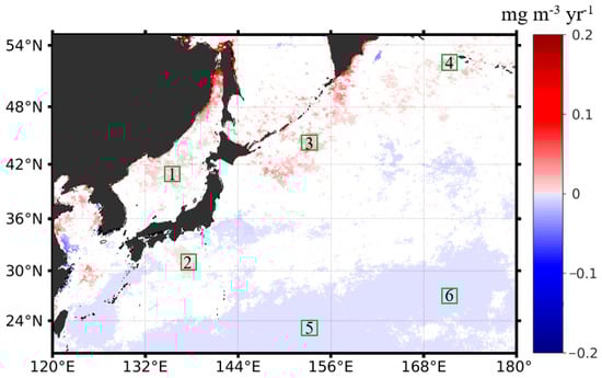
Figure 5.
The spatial distribution of the interannual changing rates (unit: mg m−3 yr−1) of Chl-a in the northwest Pacific, based on the monthly Chl-a anomalies in the period of 1997–2020, with warm colors suggesting a Chl-a increase (i.e., positive trends) and cold colors suggesting a Chl-a decrease (i.e., negative trends). Note that only data that passed the confident tests (p < 0.05) were shown; the areas in white mean that the Chl-a had no significant interannual trends in the study period. The six subregions outlined in a 2° × 2° box (i.e., boxes of 1–6 outlined in green) were selected for further investigation of the contrasting Chl-a interannual dynamics (i.e., positive vs. negative trends).
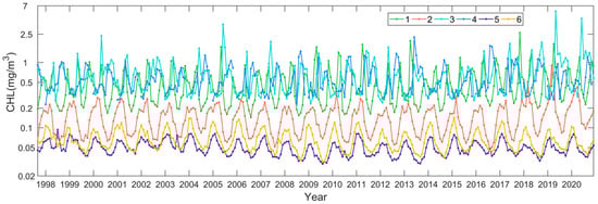
Figure 6.
Interannual data time series of Chl-a in the six subregions in the northwest Pacific (see Figure 5 for the specified locations).
In the subpolar waters of the northwest Pacific, where the red belt with positive Chl-a trends is located, the phytoplankton tended to accumulate more biomass in the study period of 1997–2020. Specifically, in the East Sea at high latitudes (>48°N), the Chl-a had a much higher increasing rate of 0.06 mg m−3 yr−1, consistent with the findings of Park et al. (2022). In the offshore waters of the East Sea (represented by subregion 1 in Figure 5), the Chl-a had an increasing trend of 0.01 mg m−3 yr−1, on average. Overall, the Chl-a showed significant increasing trends in most areas of the East Sea, except for the southern East Sea, consistent with the published results (Park et al., 2022). In the China Seas, including Bohai and Yellow Sea, the Chl-a also showed some increases. Initiating from the marginal seas, continuous patches with increasing Chl-a extended towards the northeast in the northwest Pacific, forming a Chl-a belt with positive interannual changing rates. We examined the magnitude of Chl-a increasing trends around the Kuril Island chains off the Sea of Okhotsk (subregion 3) and in the far northeast open waters (subregion 4). Off the Sea of Okhotsk, the patches with positive Chl-a trends were continuous in space off the chain of islands, and the Chl-a had an annual increasing rate of ~0.02 mg m−3 yr−1. Further toward the northeast, the patches with increasing Chl-a continued off the south of the Bering Sea. Based on the Chl-a interannual changing rates in subregion 4, we found that the Chl-a in the high-latitude open oceans had an annual increasing trend of 0.01 mg m−3 yr−1.
Unlike the annual increasing patterns in Chl-a in most of the subpolar waters, the Chl-a in the subtropical ocean waters showed little or very weak decreasing trends (e.g., <−0.0006 mg m−3 yr−1). Off the East China Sea and the south of the Japan Island (i.e., subregion 2), there were distinct small patches with small increasing rates of Chl-a; however, they did not show any spatial connection with adjacent waters, where either no or very weak decreasing interannual signals in Chl-a were observed. The increasing rate of the Chl-a off the Japan Island (i.e., represented by subregion 2) was pretty small at 0.002 mg m−3 yr−1. In the subtropical oligotrophic gyres, particularly southward of the latitude of 30°N, there was a large patch of waters with decreasing interannual changing rates (e.g., <−0.0006 mg m−3 yr−1) in Chl-a. However, these Chl-a interannual decreases were very small. Taking the subregions 5 and 6 as the representatives, we found that the Chl-a decreasing trends in these regions were −0.00035 and −0.0004 mg m−3 yr−1.
4. Discussion
4.1. Seasonal Dynamics of Phytoplankton Chl-a
As described in Section 3.1, the phytoplankton Chl-a in the northwest Pacific showed large seasonal variabilities, which reflected the seasonal growth of phytoplankton. The mechanisms of the seasonal phytoplankton blooms in the global oceans have been studied for over 60 years. Solar light radiation, nutrients availability, seawater temperature, marine heatwaves, mixed layer depth, zooplankton grazing pressure, and the atmospheric conditions were reported to be the environmental parameters that drive the seasonal variability of phytoplankton growth and phenology [13,14,55,56,57,58,59,60,61]. Most of the published studies focused on the other ocean basins or marginal seas [23,38,43,44,45,61,62]; here, we investigated the seasonal dynamics of the phytoplankton Chl-a in the northwest Pacific. Similar to the spatial patterns identified in the North Atlantic [61,62], the Chl-a from the ocean color in the northwest Pacific showed different seasonal cycles in the mid-high- (i.e., subpolar) and low-latitude (i.e., subtropical) waters, with blooms in both spring and fall and a single bloom in spring, respectively (Figure 3 and Figure 4).
In the subpolar waters, the mixed layer depth modulated the initiation of the spring and fall blooms of the phytoplankton [61]. In spring, with the warming of surface waters, more light penetrated into the euphotic zone as a consequence of the ocean stratification together with the sufficient nutrient support in the upper oceans (i.e., wind-driven mixing in wintertime) [63,64], and spring blooms were triggered. The quick growth of phytoplankton rapidly consumed the nutrients in the euphotic zone. In summertime, the mixed layer depths were very shallow, and strong stratification blocked the nutrients supply from the depth. With the additional increasing grazing pressure of zooplankton, as a result, the phytoplankton biomass kept at low levels. In fall, the vertical mixing started to prevail, which alleviated the nutrients (e.g., iron, phosphorus, nitrate) limitation to some extent (i.e., nutrients entrainment from the subsurface); yet, the light conditions and water temperature still favored the phytoplankton growth during this time interval; thus, all these supporting environmental conditions helped the phytoplankton to bloom again [62], but the magnitudes of the fall blooms were much smaller than those in the spring (Figure 4). In wintertime, the cold and strong winter mixing deepened the mixed layer depth, and the mixed substances in the water column limited solar light penetration, leading to the seasonal minima in the phytoplankton biomass [64].
In the subtropical ocean waters at low latitudes in the northwest Pacific, only spring blooms were observed from the satellite-derived Chl-a. The onset of the spring blooms was similar to the spring blooms in the subpolar oceans. With sufficient nutrients brought to the ocean surface by previous wintertime mixing, increasing stratification and solar irradiance, as well as the warm seawater temperature, which promoted the enzyme-catalyzed metabolisms of the phytoplankton, the spring bloom occurred [61]. The termination of the spring blooms was mainly controlled by nutrient depletion and zooplankton grazing [62]. However, no phytoplankton blooms were observed in other seasons in the subtropical waters. High seawater temperatures and inhibited vertical mixing seem to be the main factors that limited the phytoplankton growth in the summer and fall, resulting in a single seasonal bloom in the subtropical waters. Specifically, based on Vant Hoff’s Law, the phytoplankton growth could be accelerated with an exponential increase in cell division rates in response to increasing temperatures within a certain temperature range [55,65]. Once the seawater temperature reached beyond the tolerating range, phytoplankton growth would be dampened [66]. It is noted that, with the seasonal warming, the seawater temperature in the subtropical gyres of the northwest Pacific could reach >30 °C in summer and fall, which seems to constrain the phytoplankton growth during this period.
In addition to the common environmental forcings that define the different seasonal bloom characteristics, the local oceanic environment also plays an important role in modulating the seasonal patterns of the phytoplankton biomass in the northwest Pacific (as shown in Figure 3). For example, the Primorye coast of the East Sea was supplied with ice-melting low-salinity water from the Liman cold current in March [67]. As such, the seawater stratified at an earlier stage, which caused the spring bloom to occur earlier (Figure 3). In contrast, in the Sea of Okhotsk, under the influence of the East Sakhalin Current, the surface nitrate reservoir was greatly enriched from early winter to the next spring; however, due to the postponed warming of the sea surface, which started in April, the rapid increase in phytoplankton Chl-a was delayed to late spring [68].
4.2. Driving Factors of the Chl-a Interannual Dynamics
Based on the interannual variations of Chl-a in the study period of 1997–2020, we found that the seasonal patterns of the phytoplankton blooms were stable, without any potential advancing or delaying trends in the past 23 years (Figure 4); yet, the bloom timing and durations varied to some extent over the study period. Studies show that the bloom timing could affect the bloom duration, with early phytoplankton blooms tending to last longer than late-initiated blooms, and the specific local environmental forcings drove the interannual variabilities of the phytoplankton biomass [16]. As discussed in Section 4.1, different environmental forcings, including warming and cooling, solar light penetration, wind-driven mixing, and nutrient conditions, could trigger the onset and termination of the seasonal blooms. For example, Yamada et al. [22] demonstrated that wind speed could drive the initiation of spring blooms, and weaker wind speeds could lead to an earlier development of the seasonal thermocline. Hereafter, using a Gaussian fitting curve between the phytoplankton phenology matrix and the wind speed, Yamada et al. [33] simulated the inter-annual variability of the spring phytoplankton blooms in the southern East Sea, which further demonstrated the strong dependency between the bloom timing and wind strength and the effects of climate changes (e.g., ENSO) on the wind variabilities.
The analyses of the monthly Chl-a anomalies showed that the phytoplankton biomass had significant increasing trends in some regions of the northwest Pacific (Figure 5). To have a better understanding of the interannual variabilities of the phytoplankton Chl-a in the northwest Pacific, we thoroughly examined the interannual variations of seawater temperature (i.e., from SST), the solar light conditions (i.e., from PAR), the wind and mixing conditions (i.e., from SSW), and the nutrient conditions (i.e., from SSN), as well as the climate conditions (i.e., from MEI, AOI, PDO).
As mentioned above, SST not only influences the phytoplankton metabolism but also affects surface stratification. The strength of the surface stratification controls the intensity of vertical mixing, which in turn affects the development of the surface mixed layer and the entrainment of nutrients at the base of the mixed layer [69]. Figure 7a shows the spatial distribution of the interannual changing rates of SST between 2002 and 2020. It was found that the SST was increasing in most of the northwest Pacific, which suggests that the stratification of the northwest Pacific was getting stronger in the past two decades, consistent with the published studies [42,70]. Still, it was noted that the SST showed little interannual changes in the northeast Sea and the open ocean waters west of 168°E and north of 36°N, with small patches of weak decreasing trends in the northern East Sea and off the Japan Island in the Pacific. The interannual SST dynamics in the northern East Sea were attributed to the warming of the Arctic Ocean in the winter [38,70]. Overall, the general SST increasing trends in the northwest Pacific should set a stronger barrier (i.e., enhanced stratification) to inhibit the nutrient transport from the subsurface, and the phytoplankton Chl-a should have been decreasing in response to the reduced nutrient supplies. Indeed, we found weak decreasing trends in Chl-a in the subtropical waters (i.e., equatorward of 36°N; see Figure 5). However, this is not the case for the subpolar waters. In these waters, we observed distinct increasing trends (i.e., the opposite phenomenon) in Chl-a, and these waters formed a belt of phytoplankton expanding from the marginal seas towards the northeast direction of the north Pacific. Statistically, for the six subregions with increasing (i.e., subregions of 1–4) and decreasing (i.e., subregions of 5–6) trends identified in the Chl-a data (see Figure 5), we found significant correlations between Chl-a and SST only in the subregions 5 and 6 (note that these two subregions were located in the subtropical waters), with R = −0.19 and R = −0.44 at p < 0.05 (see Table 1), which proved our hypothesis that the decreasing trends in Chl-a in the subtropical waters were most likely driven by the ocean warming and stronger stratification. However, for the other four subregions where Chl-a showed increasing trends, we did not find any significant correlations between Chl-a and SST. As such, we suspect that, instead of SST, other environmental forcings could potentially drive the interannual increases in the phytoplankton Chl-a in the subpolar waters.
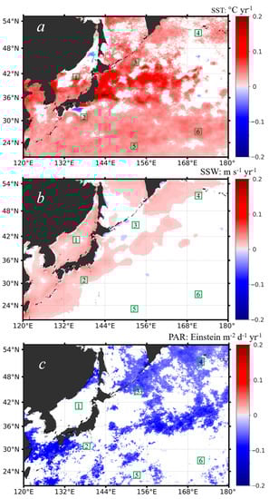
Figure 7.
The spatial distribution of the interannual changing rates of different environmental variables including SST (a), SSW (b), and PAR (c) in the northwest Pacific, based on the monthly data anomalies in the period of 1997–2020, with warm colors suggesting positive trends and cold colors suggesting negative trends. Note that only statistics at the significance level (i.e., p < 0.05) were shown; the areas in white mean that the variable had no significant trends in the study period. The six subregions outlined in a 2° × 2° box (i.e., boxes of 1–6 outlined in green) are the same as those shown in Figure 5.

Table 1.
Statistics of the correlation coefficient (R) between the Chl-a and different environmental variables (i.e., SST, PAR, SSW, and SSN) and climate indices (i.e., MEI, AOI, PDO) in the six subregions (see Figure 5 for the detailed locations). Note that the correlation analyses were based on the data time series of monthly anomalies. The statistics shown in bold and italics mean correlation coefficients at a significance level of p < 0.05.
Similarly, we further examined the interannual dynamics of SSW and PAR based on the monthly anomalies of each in the period of 1997–2020. Figure 7b shows the interannual changing rates of SSW in the northwest Pacific. The SSW showed a weak increasing pattern around the marginal seas and coastal regions and few changes far offshore in the open northwest Pacific on the eastern side. Particularly, it is noted that, corresponding to the distinct Chl-a increase off the Sea of Okhotsk (see Figure 5), the SSW did not change much along the years. Again, we examined the correlations between the interannual SSW and the interannual Chl-a based on the monthly anomalies for each of the six subregions; however, we did not find any significant relations between them. Based on the published studies, we speculated that the SSW could affect the initiation and duration of the seasonal blooms [22,33], but it was not responsible, to a large extent, for the annual increasing or decreasing trends in Chl-a. In terms of PAR, there were some slight decreasing trends (Figure 7c), which seem to be caused by the increasing anthropogenic aerosols in the atmosphere [71,72]; however, the spatial pattern of the PAR trends was quite different from that of Chl-a. From the statistical measures of R (Table 1), only subregion 6 showed a somewhat positive correlation with PAR (R = 0.17, p < 0.05), but the PAR data in this subregion had few trends, which still cannot support the Chl-a trends identified well.
For the interannual dynamics of the SSN in the northwest Pacific, extensive historical in situ SSN data were processed following a defined procedure (see Section 2.2 and Section 2.3). Figure 8a shows the SSN interannual change in the northwest Pacific in the past 40 years. Due to the data limitation in both the spatial and temporal coverage, there are lots of data gaps shown in Figure 7, even with a grid size of 2° × 2°. In general, for the areas with increasing Chl-a in the subpolar waters, where SSN data were available, the SSN tended to increase, particularly in the central East Sea (i.e., around the subregion 1). For areas with decreasing Chl-a in the subtropical waters, the SSN was decreasing. However, the SSN data were very limited. For example, in the open ocean waters along the Chl-a increasing belt, unfortunately, there were few SSN data to support trend detections. It is noted that the SSN around the Japan Island showed some pixelized increasing and decreasing trends, indicating more complicated SSN dynamics in this area, which could be caused by the data heterogeneity in temporal distributions between 1980 and 2020 (Figure 8b). Specifically, for the six subregions selected in Figure 5, the corresponding SSN was only available for subregion 5. For a statistical measure, we expanded the targeted subregions two times larger (i.e., expanded to 6° × 6°, see the yellow boxes in Figure 8). Still, no SSN data were available for the expanded subregions of 4 and 6. For the subregions of 1, 2, and 3, where Chl-a had significant increasing trends, and subregion 5, where Chl-a had significant decreasing trends, we found significant positive correlations between Chl-a and SSN, with R = 0.58, R = 0.32, R = 0.40, and R = 0.51, respectively, at p < 0.05 (see Table 1), suggesting the coupling of Chl-a and SSN in both the subpolar and subtropical oceans of the northwest Pacific. In the open ocean waters, surface nutrients are either from the recycling of nutrients in the euphotic zone or from the entrainment of nutrients from deep waters via wintertime mixing. With the ocean warming identified in Figure 7a, the nutrients transported from the subsurface via vertical mixing would be reduced to some extent. The increasing abundance of SSN in the subpolar northwest Pacific (Figure 8) indicates that there could be external nitrate inputs in these regions, such as anthropogenic nitrogen deposition from the atmosphere, which was analyzed in [47,48]. However, more in situ SSN data are needed to constrain the interannual variabilities of SSN in the northwest Pacific.
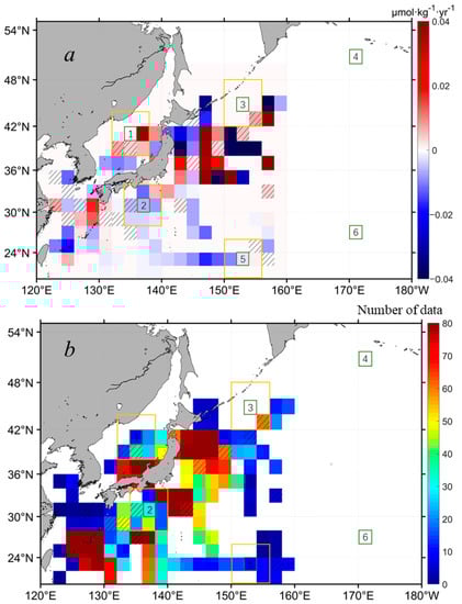
Figure 8.
(a) The spatial distribution of the interannual changing rates of SSN in the northwest Pacific, based on the monthly means of in situ SSN with a grid size of 2° × 2° in the period of 1980–2020 (see Section 2.3 for more details). Warm colors suggest positive trends and cold colors suggest negative trends. Note that pixels with cross lines mean insignificant statistics at p > 0.05, and pixels in white mean that no data are available. (b) The number of monthly data used to calculate the interannual changing rates of SSN in (a). The six subregions outlined in a 2° × 2° box (i.e., boxes of 1–6 outlined in green) are the same as those shown in Figure 5. The SSN anomalies within the yellow boxes around the subregions of 1, 2, 3, and 5 were extracted for statistical measures of correlations with the associated Chl-a anomalies.
Finally, we investigated the effects of climate variabilities on the interannual changes in Chl-a in the northwest Pacific. In general, the global climate indices on annual and decadal scales seemed to have limited effects on the Chl-a increasing or decreasing trends in the northwest Pacific; this was at least the case for the six representative subregions. Still, we found somewhat significant but weak correlations with AOI and MEI in subregions 2 and 4 (see Table 1). Specifically, for the Chl-a off the Japan Island (subregion 2), it showed some correlation with AOI at R = 0.17 (at p < 0.05), suggesting the positive effects of the Arctic Ocean Oscillation on the Chl-a interannual variability in this spot. When the AOI was in a warm phase, the Chl-a anomalies in subregion 2 tended to be positive, and vice versa. However, further investigation is needed to explore the remote control of the AOI on Chl-a in the northwest Pacific. Similarly, the Chl-a in subregion 4 were found to be negatively correlated with MEI (R = −0.13, at p < 0.05), indicating the regional effects of ENSO on Chl-a interannual dynamics.
4.3. Implication
The variabilities of the phytoplankton biomass, particularly on long-term scales, could have a big impact on the oceanic uptake of atmospheric CO2 and the effective carbon export to the ocean interior. The favorable conditions of phytoplankton growth tend to be vulnerable under global climate change and global warming. In this study, using the ocean color satellite Chl-a data records in the period of 1997–2020, we examined the seasonal and interannual variabilities of the phytoplankton Chl-a in the northwest Pacific and revealed the long-term trends of Chl-a in the past 23 years, with spatial divergence. Despite the intrinsic uncertainties involved in the satellite Chl-a retrievals, small but significant trends in Chl-a were observed. It was found that both SST and SSN were the dominant drivers of the interannual dynamics of Chl-a. The warming of seawater tended to inhibit the nutrient transport from deep waters, thus limiting phytoplankton growth and biomass in the euphotic zone. Yet, in the subpolar waters under the downwind of the Asian continent winds, the increase in phytoplankton Chl-a was most likely driven by external nutrient supplies. Still, it should be noted that the SSN interannual dynamics analyzed in this study were quite limited on both spatial and temporal scales, and finer SSN data products (e.g., SSN from satellite remote sensing) as well as other nutrient data reservoirs would be helpful in constraining the findings in this study. Furthermore, with sufficient field Chl-a measurements available in the future, the uncertainties of the satellite Chl-a should be assessed for each year for a more detailed quantification of the interannual trends in Chl-a.
5. Conclusions
In this study, our investigation of the phytoplankton biomass from the ocean color Chl-a in the northwest Pacific in the past 23 years (1997–2020) suggests that: (1) the seasonal blooms were the dominant characteristics of the seasonal variabilities of the phytoplankton Chl-a, (2) there were interannual variabilities of the seasonal algal blooms in terms of seasonal Chl-a maxima and minima, and (3) the Chl-a had significant long-term increasing and decreasing trends in the subpolar and subtropical waters of the northwest Pacific, respectively. By analyzing the interannual variabilities of different environmental factors that could affect the phytoplankton growth, as well as the climate indices on different scales, we found that the negative trends in Chl-a in the subtropical waters were most likely to be induced by the surface warming, which inhibited the nutrients supplies to the upper ocean. Yet, for the subpolar waters, where a Chl-a increasing belt was identified even under surface warming, the increasing SSN tended to be the dominant factor. We speculate that there were external nitrate supplies from other sources into the upper ocean environment, for which further studies are needed in the future.
Author Contributions
Conceptualization, S.C.; Formal analysis, Y.M., S.L. and J.X.; Funding acquisition, S.C.; Methodology, S.C. and Y.M.; Project administration, S.C.; Visualization, S.C., Y.M., S.L. and J.X.; Writing—original draft, S.C.; Writing—review & editing, S.C. All authors have read and agreed to the published version of the manuscript.
Funding
This work was supported by the National Natural Science Foundation of China (42030708, 41906159, and 42276184), the Qianjiang Talent Program of Zhejiang Province (QJD2002034), and the National Key Research and Development Program of China (2021YFE0117600).
Data Availability Statement
The satellite data used in this study were accessed from the NASA Goddard Space Flight Center (http://oceancolor.gsfc.nasa.gov/, accessed on 21 March 2021) and the Remote Sensing Systems (https://www.remss.com/, accessed on 4 July 2021). The in situ nitrate data were from the World Ocean Database (https://www.ncei.noaa.gov/products/world-ocean-database, accessed on 23 May 2020), the World Ocean Atlas (https://www.ncei.noaa.gov/products/world-ocean-atlas, accessed on 12 November 2019), and the Japan Meteorological Agency (https://www.jma.go.jp/jma/indexe.html, accessed on 23 July 2020), and the climate indices data were obtained from the NOAA Physical Sciences Laboratory(https://psl.noaa.gov/enso/mei/, accessed on 19 September 2022 ), the NOAA Climate Prediction Center (https://www.cpc.ncep.noaa.gov/products/precip/CWlink/daily_ao_index/ao_index.htmlaccessed on 19 September 2022), and the NOAA National Centers for Environmental Information (https://www.ncei.noaa.gov/products/world-ocean-database, accessed on 23 May 2020).
Acknowledgments
The authors thank the NASA Goddard Space Flight Center and the Remote Sensing Systems for maintaining and providing the satellite data used in this study. The authors thank the different research groups for collecting and processing the in situ nitrate data and thank the World Ocean Database, the World Ocean Atlas, and the Japan Meteorological Agency for synthesizing and maintaining these data treasures. The authors also thank the NOAA Physical Sciences Laboratory, the NOAA Climate Prediction Center, and the NOAA National Centers for Environmental Information for providing the climate indices data. The authors thank the two anonymous reviewers for the constructive comments that helped to improve the manuscript.
Conflicts of Interest
The authors state that there was no conflict of interest involved in this study.
References
- Arteaga, L.; Pahlow, M.; Oschlies, A. Global patterns of phytoplankton nutrient and light colimitation inferred from an optimality-based model. Glob. Biogeochem. Cycles 2014, 28, 648–661. [Google Scholar] [CrossRef]
- Boyer, T.P.; Baranova, O.K.; Coleman, C.; Garcia, H.E.; Grodsky, A.; Locarnini, R.A.; Mishonov, A.V.; Paver, C.R.; Reagan, J.R.; Seidov, D.; et al. World Ocean Database 2018; AV Mishonov, Technical Ed.; NOAA Atlas NESDIS: Silver Spring, AR, USA, 2018; p. 87. [Google Scholar]
- Bryndum-Buchholz, A.; Tittensor, D.P.; Blanchard, J.L.; Cheung, W.W.L.; Coll, M.; Galbraith, E.D.; Jennings, S.; Maury, O.; Lotze, H.K. Twenty-first-century climate change impacts on marine animal biomass and ecosystem structure across ocean basins. Glob. Chang. Biol. 2019, 25, 459–472. [Google Scholar] [CrossRef] [PubMed]
- Balaguru, K.; Foltz, G.R.; Leung, L.R.; Emanuel, K.A. Global warming-induced upper-ocean freshening and the intensification of super typhoons. Nat. Commun. 2016, 7, 13670. [Google Scholar] [CrossRef] [PubMed]
- Boyce, D.G.; Lewis, M.R.; Worm, B. Global phytoplankton decline over the past century. Nature 2010, 466, 591–596. [Google Scholar] [CrossRef] [PubMed]
- Breitburg, D.; Levin, L.A.; Oschlies, A.; Grégoire, M.; Chavez, F.P.; Conley, D.J.; Garçon, V.; Gilbert, D.; Gutiérrez, D.; Isensee, K.; et al. Declining oxygen in the global ocean and coastal waters. Science 2018, 359, eaam7240. [Google Scholar] [CrossRef] [PubMed]
- Bristow, L.A.; Mohr, W.; Ahmerkamp, S.; Kuypers, M.M. Nutrients that limit growth in the ocean. Curr. Biol. 2017, 27, R474–R478. [Google Scholar] [CrossRef] [PubMed]
- Brown, C.J.; Fulton, E.A.; Hobday, A.J.; Matear, R.J.; Possingham, H.P.; Bulman, C.; Christensen, V.; Forrest, R.E.; Gehrke, P.C.; Gribble, N.A.; et al. Effects of climate-driven primary production change on marine food webs: Implications for fisheries and conservation. Glob. Chang. Biol. 2010, 16, 1194–1212. [Google Scholar] [CrossRef]
- Browning, T.J.; Liu, X.; Zhang, R.; Wen, Z.; Liu, J.; Zhou, Y.; Xu, F.; Cai, Y.; Zhou, K.; Cao, Z.; et al. Nutrient co-limitation in the subtropical Northwest Pacific. Limnol. Oceanogr. Lett. 2022, 7, 52–61. [Google Scholar] [CrossRef]
- Chen, B.; Liu, H. Relationships between phytoplankton growth and cell size in surface oceans: Interactive effects of temperature, nutrients, and grazing. Limnol. Oceanogr. 2010, 55, 965–972. [Google Scholar] [CrossRef]
- Chen, S.; Hu, C.; Barnes, B.B.; Xie, Y.; Lin, G.; Qiu, Z. Improving ocean color data coverage through machine learning. Remote Sens. Environ. 2019, 222, 286–302. [Google Scholar] [CrossRef]
- Chen, S.; Meng, Y. Phytoplankton Blooms Expanding Further Than Previously Thought in the Ross Sea: A Remote Sensing Perspective. Remote Sens. 2022, 14, 3263. [Google Scholar] [CrossRef]
- Chen, S.; Smith, W.O.; Yu, X. Revisiting the Ocean Color Algorithms for Particulate Organic Carbon and Chlorophyll-a Concentrations in the Ross Sea. J. Geophys. Res. Ocean. 2021, 126, e2021JC017749. [Google Scholar] [CrossRef]
- Chiba, S.; Batten, S.; Sasaoka, K.; Sasai, Y.; Sugisaki, H. Influence of the Pacific Decadal Oscillation on phytoplankton phenology and community structure in the western North Pacific. Geophys. Res. Lett. 2012, 39, L5603. [Google Scholar] [CrossRef]
- Cronin, M.F.; Bond, N.A.; Farrar, J.T.; Ichikawa, H.; Jayne, S.R.; Kawai, Y.; Konda, M.; Qiu, B.; Rainville, L.; Tomita, H. Formation and erosion of the seasonal thermocline in the Kuroshio Extension Recirculation Gyre. Deep Sea Res. Part II Top. Stud. Oceanogr. 2013, 85, 62–74. [Google Scholar] [CrossRef]
- Diaz, B.P.; Ben Knowles, B.; Johns, C.T.; Laber, C.P.; Bondoc, K.G.V.; Haramaty, L.; Natale, F.; Harvey, E.L.; Kramer, S.J.; Bolaños, L.M.; et al. Seasonal mixed layer depth shapes phytoplankton physiology, viral production, and accumulation in the North Atlantic. Nat. Commun. 2021, 12, 6634. [Google Scholar] [CrossRef] [PubMed]
- Di Lorenzo, E.; Schneider, N.; Cobb, K.M.; Franks, P.J.S.; Chhak, K.; Miller, A.J.; McWilliams, J.C.; Bograd, S.J.; Arango, H.; Curchitser, E.; et al. North Pacific Gyre Oscillation links ocean climate and ecosystem change. Geophys. Res. Lett. 2008, 35, L08607. [Google Scholar] [CrossRef]
- Friedland, K.D.; Stock, C.; Drinkwater, K.F.; Link, J.S.; Leaf, R.T.; Shank, B.V.; Rose, J.M.; Pilskaln, C.H.; Fogarty, M.J. Pathways be-tween primary production and fisheries yields of large marine ecosystems. PLoS ONE 2012, 7, e28945. [Google Scholar] [CrossRef]
- Friedland, K.D.; Mouw, C.B.; Asch, R.G.; Ferreira, A.S.A.; Henson, S.; Hyde, K.J.W.; Morse, R.E.; Thomas, A.C.; Brady, D.C. Phenology and time series trends of the dominant seasonal phytoplankton bloom across global scales. Glob. Ecol. Biogeogr. 2018, 27, 551–569. [Google Scholar] [CrossRef]
- Fu, W.; Randerson, J.T.; Moore, J.K. Climate change impacts on net primary production (NPP) and export pro-duction (EP) regulated by increasing stratification and phytoplankton community structure in the CMIP5 models. Biogeosciences 2016, 13, 5151–5170. [Google Scholar] [CrossRef]
- Gaube, P.; Chelton, D.B.; Strutton, P.G.; Behrenfeld, M.J. Satellite observations of chlorophyll, phytoplankton biomass, and Ekman pumping in nonlinear mesoscale eddies. J. Geophys. Res. Ocean. 2013, 118, 6349–6370. [Google Scholar] [CrossRef]
- Gittings, J.A.; Raitsos, D.E.; Racault, M.F.; Brewin, R.J.; Pradhan, Y.; Sathyendranath, S.; Platt, T. Seasonal phytoplankton blooms in the Gulf of Aden revealed by remote sensing. Remote Sens. Environ. 2017, 189, 56–66. [Google Scholar]
- Harid, R.; Demarcq, H.; Keraghel, M.-A.; Ait-Kaci, M.; Zerrouki, M.; Bachari, N.-E.; Houma, F. Spatio-temporal variability of a chlorophyll-a based biomass index and influence of coastal sources of enrichment in the Algerian Basin. Cont. Shelf Res. 2022, 232, 104629. [Google Scholar] [CrossRef]
- Henson, S.A.; Robinson, I.; Allen, J.T.; Waniek, J. Effect of meteorological conditions on interannual variability in timing and magnitude of the spring bloom in the Irminger Basin, North Atlantic. Deep Sea Res. Part I Oceanogr. Res. Pap. 2006, 53, 1601–1615. [Google Scholar] [CrossRef]
- Henson, S.A.; Cael, B.B.; Allen, S.R.; Dutkiewicz, S. Future phytoplankton diversity in a changing climate. Nat. Commun. 2021, 12, 5372. [Google Scholar] [CrossRef]
- He, X.; Bai, Y.; Pan, D.; Chen, C.-T.A.; Cheng, Q.; Wang, D.; Gong, F. Satellite views of the seasonal and interannual variability of phytoplankton blooms in the eastern China seas over the past 14 yr (1998–2011). Biogeosciences 2013, 10, 4721–4739. [Google Scholar] [CrossRef]
- Ji, X.; Verspagen, J.M.H.; Van de Waal, D.B.; Rost, B.; Huisman, J. Phenotypic plasticity of carbon fixation stimulates cyanobacterial blooms at elevated CO2. Sci. Adv. 2020, 6, eaax2926. [Google Scholar] [CrossRef]
- Joo, H.; Lee, D.; Kang, J.J.; Lee, J.H.; Jeong, J.Y.; Son, S.H.; Kwon, J.-I.; Lee, S.H. Inter-annual variation of the annual new production of phytoplankton in the southwestern East/Japan Sea estimated from satellite-derived surface nitrate concentration. J. Coast. Res. 2018, 85, 336–340. [Google Scholar] [CrossRef]
- Kim, T.-W.; Lee, K.; Najjar, R.G.; Jeong, H.-D. Increasing N Abundance in the Northwestern Pacific Ocean Due to Atmospheric Nitrogen Deposition. Science 2011, 334, 505–509. [Google Scholar] [CrossRef]
- Kim, I.-N.; Lee, K.; Gruber, N.; Karl, D.M.; Bullister, J.L.; Yang, S.; Kim, T.-W. Increasing anthropogenic nitrogen in the North Pacific Ocean. Science 2014, 346, 1102–1106. [Google Scholar] [CrossRef]
- Ko, E.; Gorbunov, M.Y.; Jung, J.; Joo, H.M.; Lee, Y.; Cho, K.H.; Yang, E.J.; Kang, S.H.; Park, J. Effects of nitrogen limitation on phytoplankton physiology in the western Arctic Ocean In summer. J. Geophys. Res. Ocean. 2020, 125, e2020JC016501. [Google Scholar] [CrossRef]
- Kwiatkowski, L.; Torres, O.; Bopp, L.; Aumont, O.; Chamberlain, M.; Christian, J.R.; Dunne, J.P.; Gehlen, M.; Ilyina, T.; John, J.G.; et al. Twenty-first century ocean warming, acidification, deoxygenation, and upper-ocean nutrient and primary production decline from CMIP6 model projections. Biogeosciences 2020, 17, 3439–3470. [Google Scholar] [CrossRef]
- Lee, J.H.; Lee, D.; Kang, J.J.; Joo, H.T.; Lee, J.H.; Lee, H.W.; Ahn, S.H.; Kang, C.K.; Lee, S.H. The effects of different environmental factors on the biochemical composition of particulate organic matter in Gwangyang Bay, South Korea. Biogeosciences 2017, 14, 1903–1917. [Google Scholar] [CrossRef]
- Lee, E.-Y.; Park, K.-A. Change in the Recent Warming Trend of Sea Surface Temperature in the East Sea (Sea of Japan) over Decades (1982–2018). Remote Sens. 2019, 11, 2613. [Google Scholar] [CrossRef]
- Lee, J.-Y.; Kang, D.-J.; Kim, I.-N.; Rho, T.; Lee, T.; Kang, C.-K.; Kim, K.-R. Spatial and temporal variability in the pelagic ecosystem of the East Sea (Sea of Japan): A review. J. Mar. Syst. 2009, 78, 288–300. [Google Scholar] [CrossRef]
- Lewis, K.M.; Arntsen, A.E.; Coupel, P.; Joy-Warren, H.; Lowry, K.E.; Matsuoka, A.; Mills, M.M.; van Dijken, G.L.; Selz, V.; Arrigo, K.R. Photoacclimation of Arctic Ocean phytoplankton to shifting light and nutrient limitation. Limnol. Oceanogr. 2019, 64, 284–301. [Google Scholar] [CrossRef]
- Li, G.; Cheng, L.; Zhu, J.; Trenberth, K.E.; Mann, M.E.; Abraham, J.P. Increasing ocean stratification over the past half-century. Nat. Clim. Chang. 2020, 10, 1116–1123. [Google Scholar] [CrossRef]
- Martinez, E.; Antoine, D.; D’Ortenzio, F.; Montégut, C.D.B. Phytoplankton spring and fall blooms in the North Atlantic in the 1980s and 2000s. J. Geophys. Res. Earth Surf. 2011, 116, C11029. [Google Scholar] [CrossRef]
- Miao, Z.; Yang, D. Solar light, seawater temperature, and nutrients, which one is more important in affecting phytoplankton growth? Chin. J. Oceanol. Limnol. 2009, 27, 825–831. [Google Scholar] [CrossRef]
- Navarro, G.; Caballero, I.; Prieto, L.; Vázquez, A.; Flecha, S.; Huertas, I.E.; Ruiz, J. Seasonal-to-interannual variability of chlorophyll-a bloom timing associated with physical forcing in the Gulf of Cádiz. Adv. Space Res. 2012, 50, 1164–1172. [Google Scholar] [CrossRef]
- Park, K.-A.; Kim, K.; Cornillon, P.C.; Chung, J.Y. Relationship between satellite-observed cold water along the Primorye coast and sea ice in the East Sea (the Sea of Japan). Geophys. Res. Lett. 2006, 33, L10602. [Google Scholar] [CrossRef]
- Park, J.; Kim, J.; Kim, H.; Hwang, J.; Jo, Y.; Lee, S.H. Environmental Forcings on the Remotely Sensed Phytoplankton Bloom Phenology in the Central Ross Sea Polynya. J. Geophys. Res. Ocean. 2019, 124, 5400–5417. [Google Scholar] [CrossRef]
- Park, J.-E.; Park, K.-A.; Kang, C.-K.; Kim, G. Satellite-Observed Chlorophyll-a Concentration Variability and Its Relation to Physical Environmental Changes in the East Sea (Japan Sea) from 2003 to 2015. Estuaries Coasts 2020, 43, 630–645. [Google Scholar] [CrossRef]
- Park, K.A.; Park, J.E.; Kang, C.K. Satellite-Observed Chlorophyll-a Concentration Variability in the East Sea (Japan Sea): Seasonal Cycle, Long-Term Trend, and Response to Climate Index. Front. Mar. Sci. 2022, 80, 7570. [Google Scholar] [CrossRef]
- Riebesell, U.; Schulz, K.G.; Bellerby RG, J.; Botros, M.; Fritsche, P.; Meyerhöfer, M.; Neill, C.; Nondal, G.; Oschlies, A.; Wohlers, J.; et al. Enhanced biological carbon consumption in a high CO2 ocean. Nature 2007, 450, 545–548. [Google Scholar] [CrossRef] [PubMed]
- Rumyantseva, A.; Henson, S.; Martin, A.; Thompson, A.F.; Damerell, G.M.; Kaiser, J.; Heywood, K.J. Phytoplankton spring bloom initiation: The impact of atmospheric forcing and light in the temperate North Atlantic Ocean. Prog. Oceanogr. 2019, 178, 102202. [Google Scholar] [CrossRef]
- Sherman, E.; Moore, J.K.; Primeau, F.; Tanouye, D. Temperature influence on phytoplankton community growth rates. Glob. Biogeochem. Cycles 2016, 30, 550–559. [Google Scholar] [CrossRef]
- Shiomoto, A.; Inoue, K. Seasonal variations of size-fractionated chlorophyll a and primary production in the coastal area of Hokkaido in the Okhotsk Sea. SN Appl. Sci. 2020, 2, 1880. [Google Scholar] [CrossRef]
- Sverdrup, H.U. On Conditions for the Vernal Blooming of Phytoplankton. ICES J. Mar. Sci. 1953, 18, 287–295. [Google Scholar] [CrossRef]
- Ueyama, R.; Monger, B.C. Wind-induced modulation of seasonal phytoplankton blooms in the North Atlantic derived from satellite observations. Limnol. Oceanogr. 2005, 50, 1820–1829. [Google Scholar] [CrossRef]
- Wang, M.; Son, S.; Shi, W. Evaluation of MODIS SWIR and NIR-SWIR atmospheric correction algorithms using SeaBASS data. Remote Sens. Environ. 2009, 113, 635–644. [Google Scholar] [CrossRef]
- Yamada, K.; Ishizaka, J.; Yoo, S.; Kim, H.C.; Chiba, S. Seasonal and interannual variability of sea surface chlorophyll a concentration in the Japan/East Sea (JES). Prog. Oceanogr. 2004, 61, 193–211. [Google Scholar] [CrossRef]
- Yamada, K.; Ishizaka, J. Estimation of interdecadal change of spring bloom timing, in the case of the Japan Sea. Geophys. Res. Lett. 2006, 33, L02608. [Google Scholar] [CrossRef]
- Yang, Y.; Liang, S.X. On the seasonal eddy variability in the Kuroshio Extension. J. Phys. Oceanogr. 2018, 48, 1675–1689. [Google Scholar] [CrossRef]
- Yu, X.; Chen, S.; Chai, F. Remote Estimation of Sea Surface Nitrate in the California Current System From Satellite Ocean Color Measurements. IEEE Trans. Geosci. Remote Sens. 2021, 60, 4203017. [Google Scholar] [CrossRef]
- Zhou, L.; Wu, S.; Gu, W.; Wang, L.; Wang, J.; Gao, S.; Wang, G. Photosynthesis acclimation under severely fluctuating light conditions allows faster growth of diatoms compared with dinoflagellates. BMC Plant Biol. 2021, 21, 164. [Google Scholar]
- Noh, K.M.; Lim, H.-G.; Kug, J.-S. Global chlorophyll responses to marine heatwaves in satellite ocean color. Environ. Res. Lett. 2022, 17, 064034. [Google Scholar] [CrossRef]
- Mandal, S.; Susanto, R.D.; Ramakrishnan, B. On Investigating the Dynamical Factors Modulating Surface Chlorophyll-a Variability along the South Java Coast. Remote Sens. 2022, 14, 1745. [Google Scholar] [CrossRef]
- Uitz, J.; Claustre, H.; Morel, A.; Hooker, S.B. Vertical distribution of phytoplankton communities in open ocean: An assessment based on surface chlorophyll. J. Geophys. Res. Earth Surf. 2006, 111, C08005. [Google Scholar] [CrossRef]
- Gregg, W.W.; Casey, N.W. Global and regional evaluation of the SeaWiFS chlorophyll data set. Remote Sens. Environ. 2004, 93, 463–479. [Google Scholar] [CrossRef]
- Bailey, S.W.; Werdell, P.J. A multi-sensor approach for the on-orbit validation of ocean color satellite data products. Remote Sens. Environ. 2006, 102, 12–23. [Google Scholar] [CrossRef]
- Da Silva, J.C.B.; New, A.L.; Srokosz, M.A.; Smyth, T.J. On the observability of internal tidal waves in remotely-sensed ocean colour data. Geophys. Res. Lett. 2002, 29, 10-1–10-4. [Google Scholar] [CrossRef]
- Gregg, W.W.; Conkright, M.E.; Ginoux, P.; O’Reilly, J.E.; Casey, N.W. Ocean primary production and climate: Global decadal changes. Geophys. Res. Lett. 2003, 30, 1809. [Google Scholar] [CrossRef]
- Sabine, C.L.; Feely, R.A.; Gruber, N.; Key, R.M.; Lee, K.; Bullister, J.L.; Wanninkhof, R.; Wong, C.S.; Wallace, D.W.; Tilbrook, B.; et al. The oceanic sink for anthropogenic CO2. Science 2004, 305, 367–371. [Google Scholar] [CrossRef] [PubMed]
- Joo, H.; Son, S.; Park, J.W.; Kang, J.J.; Jeong, J.Y.; Lee, C.I.; Kang, C.K.; Lee, S.H. Long-term pattern of primary productivity in the East/Japan Sea based on ocean color data derived from MODIS-aqua. Remote Sens. 2015, 8, 25. [Google Scholar] [CrossRef]
- De Boyer Montegut, C.; Madec, G.; Fischer, A.S.; Lazar, A.; Iudicone, D. Mixed layer depth over the global ocean: An examination of profile data and a profile-based climatology. J. Geophys. Res. Ocean. 2004, 109, C12003. [Google Scholar] [CrossRef]
- Hu, B.; Wang, Y.; Liu, G. Long-term trends in photosynthetically active radiation in Beijing. Adv. Atmos. Sci. 2010, 27, 1380–1388. [Google Scholar] [CrossRef]
- Wang, L.; Gong, W.; Hu, B.; Lin, A.; Li, H.; Zou, L. Modeling and analysis of the spatiotemporal variations of photosynthetically active radiation in China during 1961–2012. Renew. Sustain. Energy Rev. 2015, 49, 1019–1032. [Google Scholar] [CrossRef]
- Kilpatrick, T.; Xie, S.; Miller, A.J.; Schneider, N.; Arthur, J.M. Satellite Observations of Enhanced Chlorophyll Variability in the Southern California Bight. J. Geophys. Res. Ocean. 2018, 123, 7550–7563. [Google Scholar] [CrossRef]
- Yu, Y.; Xing, X.; Liu, H.; Yuan, Y.; Wang, Y.; Chai, F. The variability of chlorophyll-a and its relationship with dynamic factors in the basin of the South China Sea. J. Mar. Syst. 2019, 200, 103230. [Google Scholar] [CrossRef]
- Siswanto, E.; Horii, T.; Iskandar, I.; Gaol, J.L.; Setiawan, R.Y.; Susanto, R.D. Impacts of Climate Changes on the Phytoplankton Biomass of the Indonesian Maritime Continent. J. Mar. Syst. 2020, 212, 103451. [Google Scholar] [CrossRef]
- Morel, A.; Berthon, J.-F. Surface pigments, algal biomass profiles, and potential production of the euphotic layer: Relationships reinvestigated in view of remote-sensing applications. Limnol. Oceanogr. 1989, 34, 1545–1562. [Google Scholar] [CrossRef]


Publisher’s Note: MDPI stays neutral with regard to jurisdictional claims in published maps and institutional affiliations. |
© 2022 by the authors. Licensee MDPI, Basel, Switzerland. This article is an open access article distributed under the terms and conditions of the Creative Commons Attribution (CC BY) license (https://creativecommons.org/licenses/by/4.0/).