


Ice Aprons in the Mont Blanc Massif (Western European Alps): Topographic Characteristics and Relations with Glaciers and Other Types of Perennial Surface Ice Features

Abstract
1. Introduction
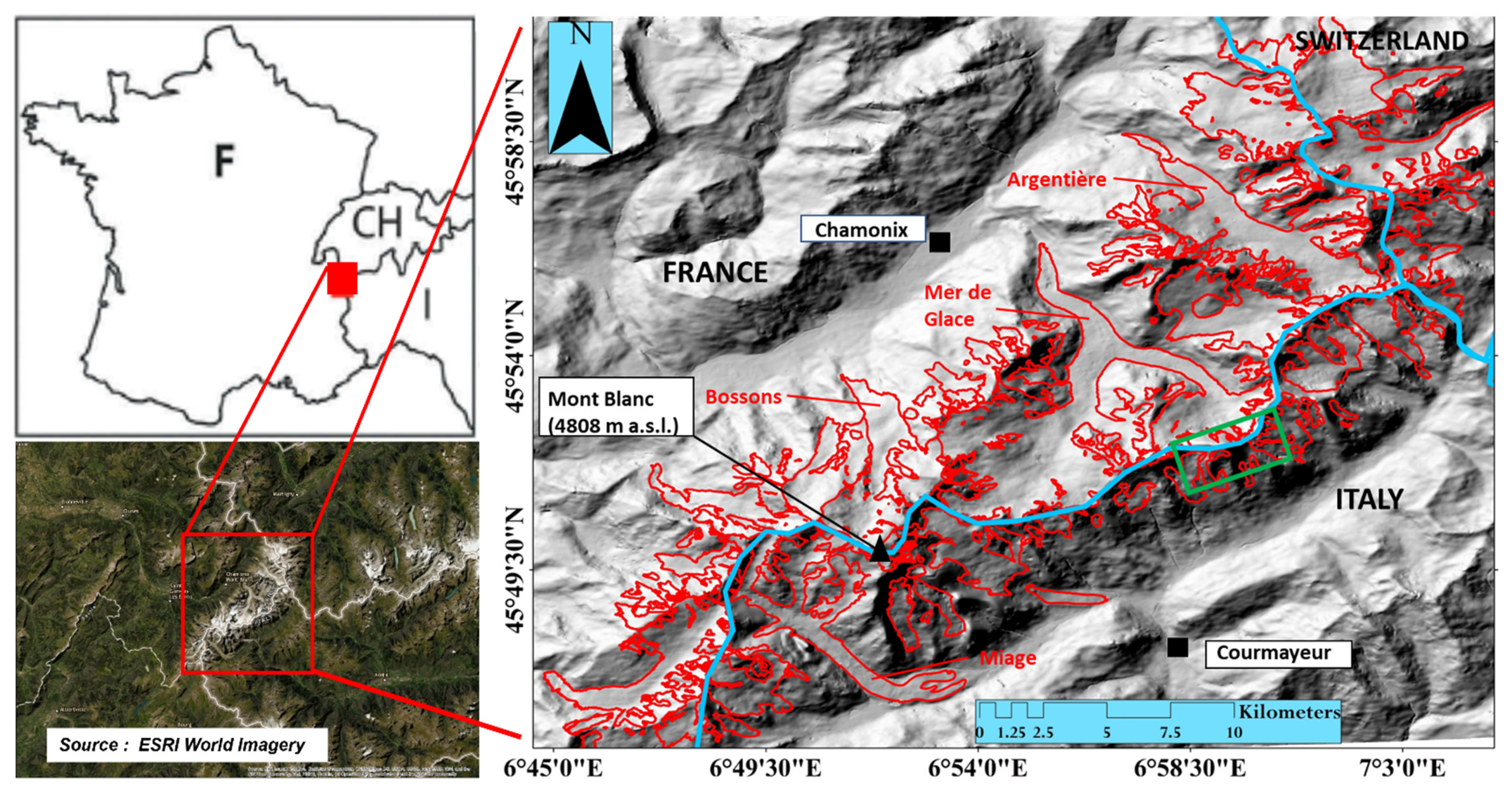
2. Study Area
3. Datasets
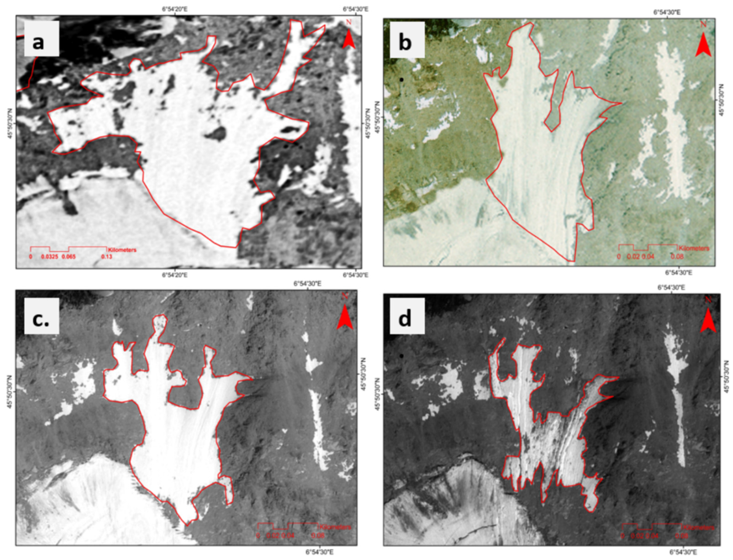
3.1. Optical Images
3.2. Digital Elevation Model
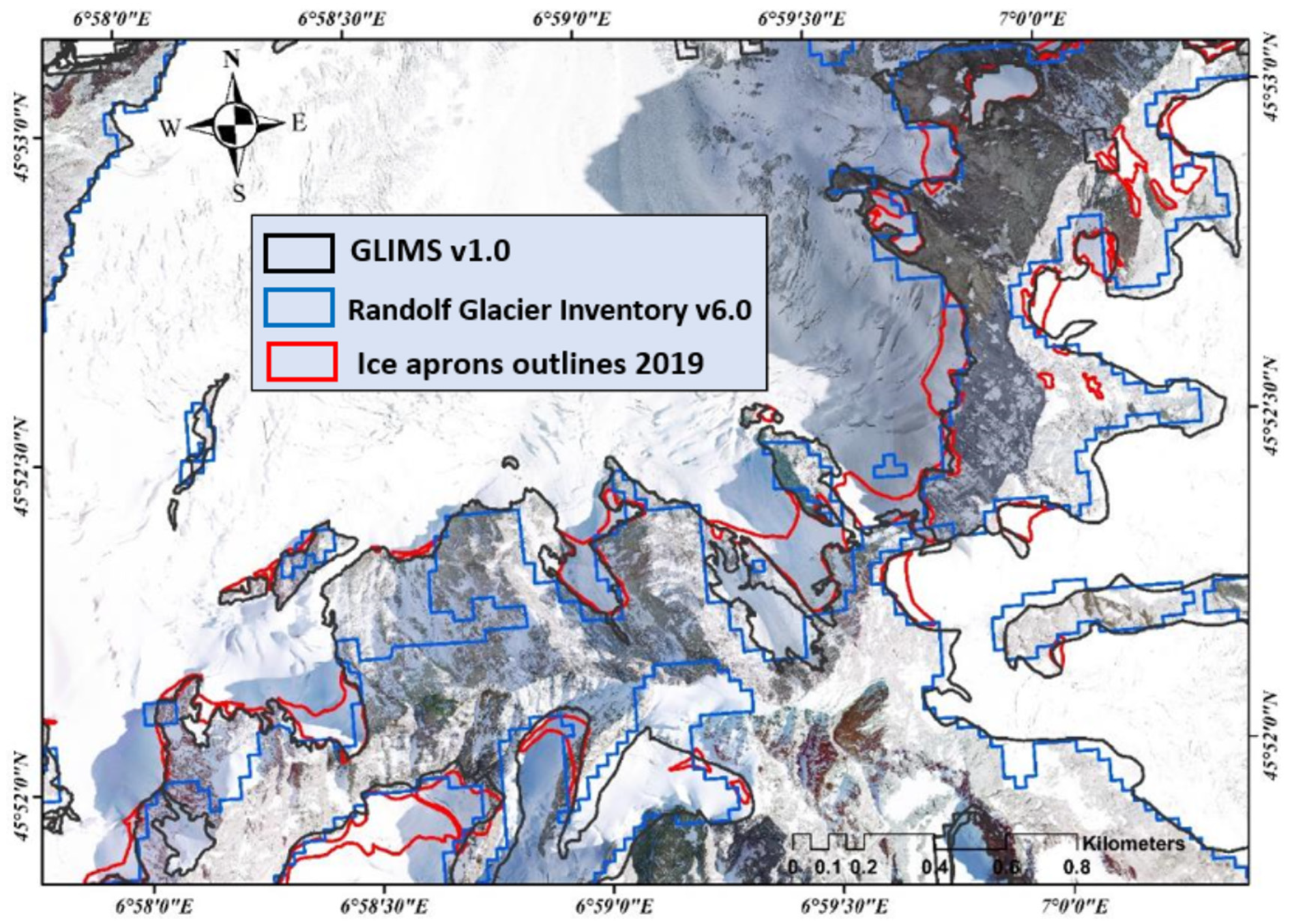
3.3. Global Glacier Inventories
4. Description and Methods
4.1. Mapping of Glaciers and Snow/Ice Bodies
4.2. Typology of Glaciers and Perennial Surface Ice Features
4.2.1. Cirque Glaciers
4.2.2. Slope Glaciers
4.2.3. Valley Glaciers
4.2.4. Glacierets
4.2.5. Alpine Ice Caps
4.2.6. Ice/Snow Covers
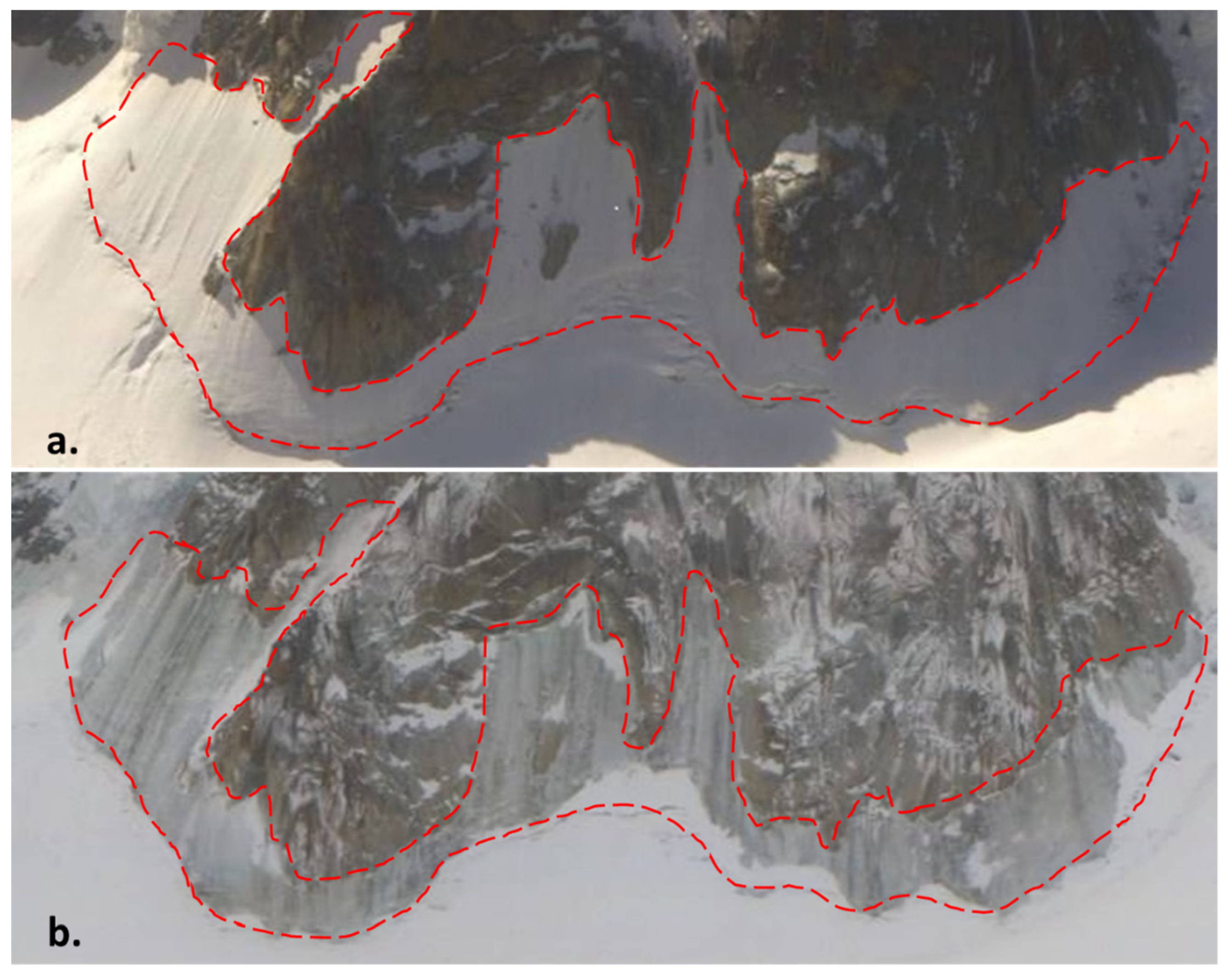
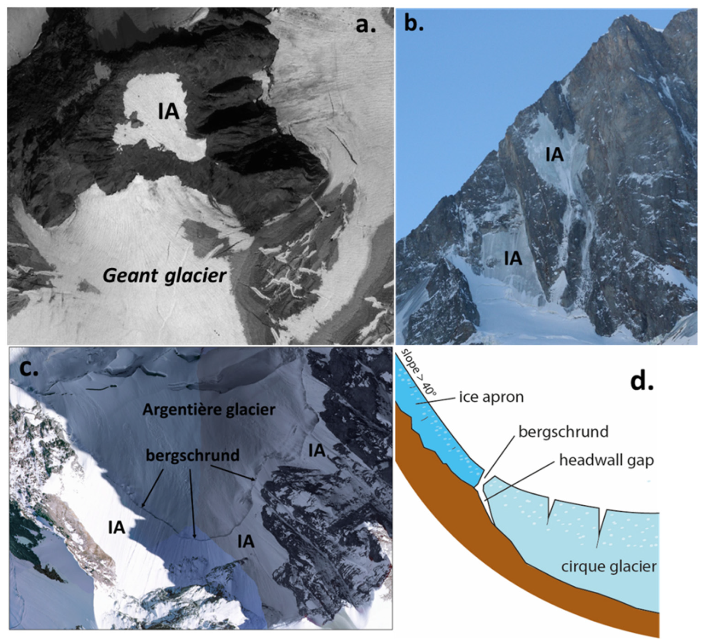
4.2.7. Ice Aprons
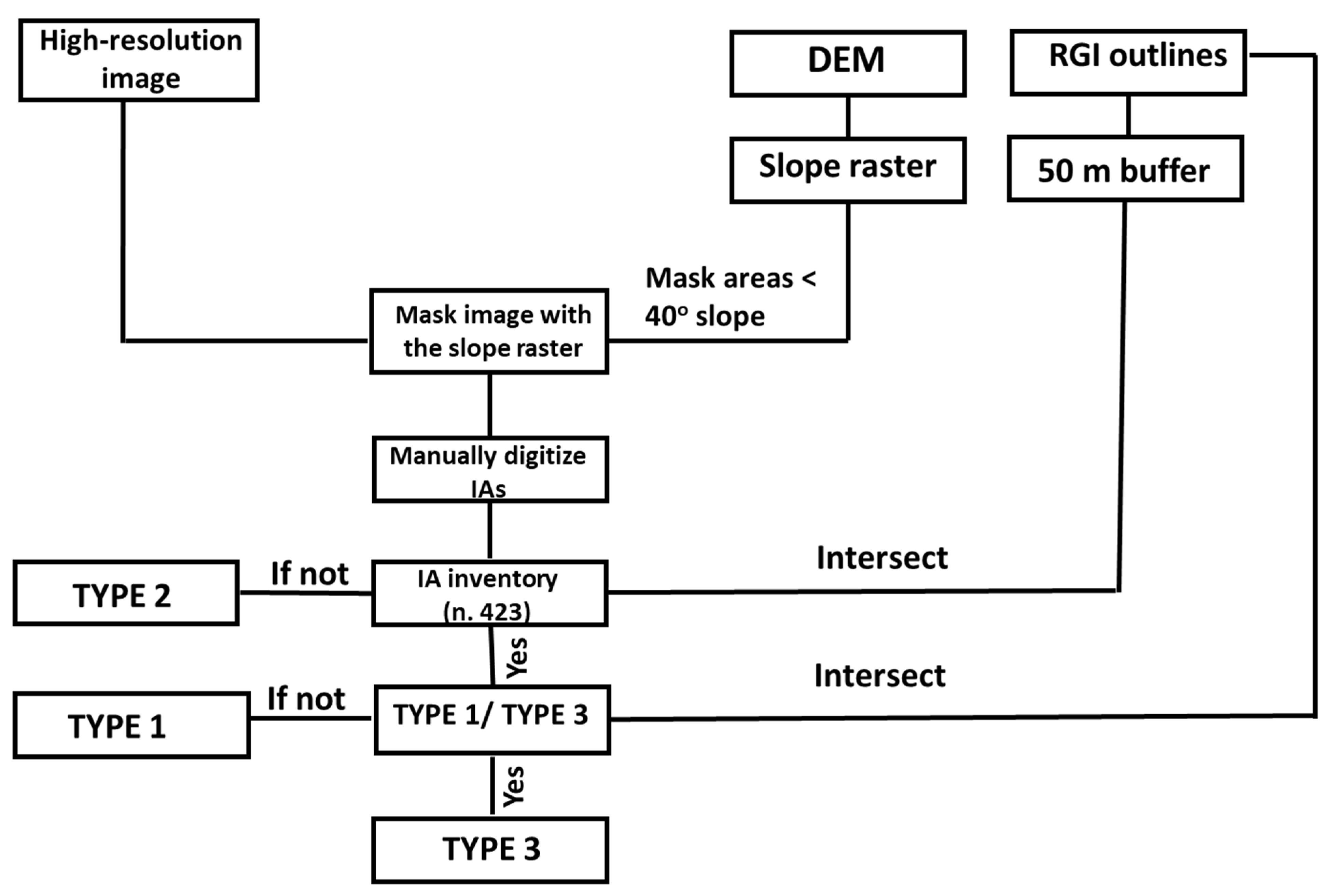
4.3. Typology of Ice Aprons
Methodology for Differentiating Types of IAs
4.4. Generation of Topographic Parameters Used to Characterize and Map Ice Aprons
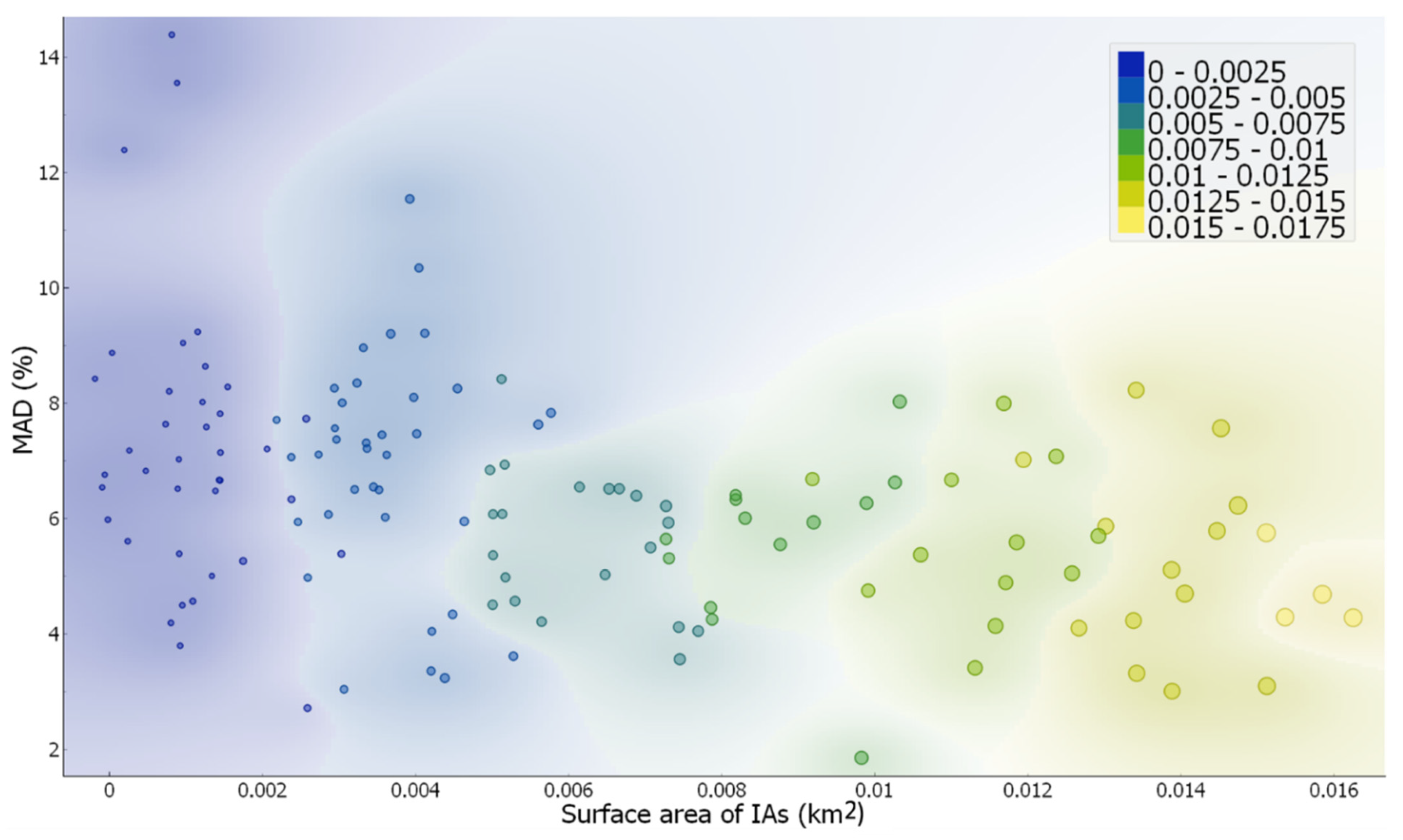
4.5. Uncertainty Associated with Mapping Ice Aprons
5. Results
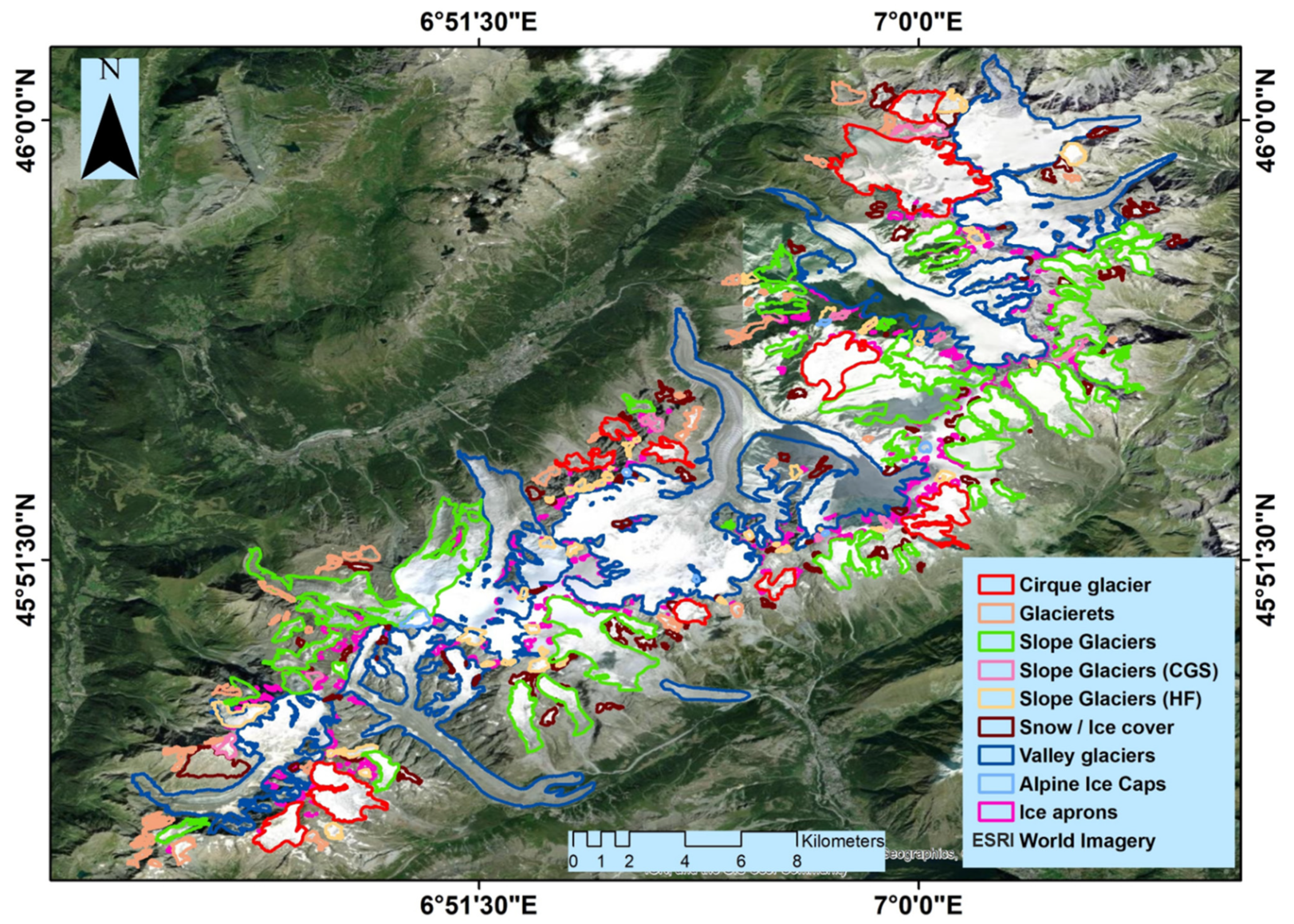
5.1. High-Resolution Glacier Typology Map of the Mont Blanc Massif
5.2. Location and Morphometric Characteristics of Ice Aprons
5.3. Ice Apron Typology and Their Distribution in the MBM
5.4. Size of Ice Aprons
6. Discussion
7. Conclusions
Author Contributions
Funding
Data Availability Statement
Acknowledgments
Conflicts of Interest
References
- Huss, M.; Fischer, M. Sensitivity of Very Small Glaciers in the Swiss Alps to Future Climate Change. Front. Earth Sci. 2016, 4, 34. [Google Scholar] [CrossRef]
- Paul, F.; Kääb, A.; Maisch, M.; Kellenberger, T.; Haeberli, W. Rapid Disintegration of Alpine Glaciers Observed with Satellite Data: Disintegration of Alpine Glaciers. Geophys. Res. Lett. 2004, 31, L21402. [Google Scholar] [CrossRef]
- Pfeffer, W.T.; Arendt, A.A.; Bliss, A.; Bolch, T.; Cogley, J.G.; Gardner, A.S.; Hagen, J.-O.; Hock, R.; Kaser, G.; Kienholz, C.; et al. The Randolph Consortium. The Randolph Glacier Inventory: A Globally Complete Inventory of Glaciers. J. Glaciol. 2014, 60, 537–552. [Google Scholar] [CrossRef]
- Benn, D.I.; Evans, D.J.A. Glaciers & Glaciation, 2nd ed.; Hodder Education: London, UK, 2010. [Google Scholar]
- Jost, G.; Moore, R.D.; Menounos, B.; Wheate, R. Quantifying the Contribution of Glacier Runoff to Streamflow in the Upper Columbia River Basin, Canada. Hydrol. Earth Syst. Sci. 2012, 16, 849–860. [Google Scholar] [CrossRef]
- Sanders, J.W.; Cuffey, K.M.; Moore, J.R.; MacGregor, K.R.; Kavanaugh, J.L. Periglacial Weathering and Headwall Erosion in Cirque Glacier Bergschrunds. Geology 2012, 40, 779–782. [Google Scholar] [CrossRef]
- Seppi, R.; Zanoner, T.; Carton, A.; Bondesan, A.; Francese, R.; Carturan, L.; Zumiani, M.; Giorgi, M.; Ninfo, A. Current Transition from Glacial to Periglacial Processes in the Dolomites (South-Eastern Alps). Geomorphology 2015, 228, 71–86. [Google Scholar] [CrossRef]
- Kuhn, M. The Mass Balance of Very Small Glaciers. Z. Für Gletsch. Und Glazialgeol. 1995, 31, 171–179. [Google Scholar]
- Triglav-Čekada, M.; Gabrovec, M. Documentation of Triglav Glacier, Slovenia, Using Non-Metric Panoramic Images. Ann. Glaciol. 2013, 54, 80–86. [Google Scholar] [CrossRef]
- Marti, R.; Gascoin, S.; Houet, T.; Ribière, O.; Laffly, D.; Condom, T.; Monnier, S.; Schmutz, M.; Camerlynck, C.; Tihay, J.P.; et al. Evolution of Ossoue Glacier (French Pyrenees) since the End of the Little Ice Age. Cryosphere 2015, 9, 1773–1795. [Google Scholar] [CrossRef]
- Guillet, G.; Ravanel, L. Variations in Surface Area of Six Ice Aprons in the Mont-Blanc Massif since the Little Ice Age. J. Glaciol. 2020, 66, 777–789. [Google Scholar] [CrossRef]
- Fischer, M.; Huss, M.; Barboux, C.; Hoelzle, M. The New Swiss Glacier Inventory SGI2010: Relevance of Using High-Resolution Source Data in Areas Dominated by Very Small Glaciers. Arct. Antarct. Alp. Res. 2014, 46, 933–945. [Google Scholar] [CrossRef]
- Capt, M.; Bosson, J.-B.; Fischer, M.; Micheletti, N.; Lambiel, C. Decadal Evolution of a Very Small Heavily Debris-Covered Glacier in an Alpine Permafrost Environment. J. Glaciol. 2016, 62, 535–551. [Google Scholar] [CrossRef]
- Jones, D.B.; Harrison, S.; Anderson, K.; Betts, R.A. Mountain Rock Glaciers Contain Globally Significant Water Stores. Sci. Rep. 2018, 8, 2834. [Google Scholar] [CrossRef] [PubMed]
- Jones, D.B.; Harrison, S.; Anderson, K.; Whalley, W.B. Rock Glaciers and Mountain Hydrology: A Review. Earth-Sci. Rev. 2019, 193, 66–90. [Google Scholar] [CrossRef]
- Armstrong, T.; Roberts, B.; Swithinbank, C. Illustrated Glossary of Snow and Ice; Scott Polar Research Institute: Cambridge, UK, 1973. [Google Scholar]
- Singh, V.P.; Singh, P.; Haritashya, U.K. Encyclopedia of Snow, Ice and Glaciers; The Encyclopedia of Earth Sciences Series; Springer: Dordrecht, The Netherlands; London, UK, 2011. [Google Scholar]
- Mourey, J.; Marcuzzi, M.; Ravanel, L.; Pallandre, F. Effects of Climate Change on High Alpine Mountain Environments: Evolution of Mountaineering Routes in the Mont Blanc Massif (Western Alps) over Half a Century. Arct. Antarct. Alp. Res. 2019, 51, 176–189. [Google Scholar] [CrossRef]
- Rebuffat, G. Le Massif du Mont-Blanc—Les 100 plus Belles Courses, 238th ed.; Denoël: Paris, France, 1973. [Google Scholar]
- Ravanel, L.; Deline, P. A Network of Observers in the Mont-Blanc Massif to Study Rockfall from High Alpine Rockwalls. Geogr. Fis. E Din. Quat. 2013, 36, 151–158. [Google Scholar] [CrossRef]
- Ravanel, L.; Magnin, F.; Deline, P. Impacts of the 2003 and 2015 Summer Heatwaves on Permafrost-Affected Rock-Walls in the Mont Blanc Massif. Sci. Total Environ. 2017, 609, 132–143. [Google Scholar] [CrossRef]
- Guillet, G.; Preunkert, S.; Ravanel, L.; Montagnat, M.; Friedrich, R. Investigation of a Cold-Based Ice Apron on a High-Mountain Permafrost Rock Wall Using Ice Texture Analysis and Micro-14C Dating: A Case Study of the Triangle Du Tacul Ice Apron (Mont Blanc Massif, France). J. Glaciol. 2021, 67, 1205–1212. [Google Scholar] [CrossRef]
- Konrad, H.; Bohleber, P.; Wagenbach, D.; Vincent, C.; Eisen, O. Determining the Age Distribution of Colle Gnifetti, Monte Rosa, Swiss Alps, by Combining Ice Cores, Ground-Penetrating Radar and a Simple Flow Model. J. Glaciol. 2013, 59, 179–189. [Google Scholar] [CrossRef]
- Preunkert, S.; Legrand, M.; Kutuzov, S.; Ginot, P.; Mikhalenko, V.; Friedrich, R. The Elbrus (Caucasus, Russia) Ice Core Glaciochemistry Toreconstruct Anthropogenic Emissions in Central Europe: The Case Ofsulfate; European Geosciences Union: Munich, Germany, 2019. [Google Scholar] [CrossRef]
- Helfricht, K.; Lehning, M.; Sailer, R.; Kuhn, M. Local Extremes in the Lidar-derived Snow Cover of Alpine Glaciers. Geogr. Ann. Ser. A Phys. Geogr. 2015, 97, 721–736. [Google Scholar] [CrossRef]
- Andreassen, L.M.; Elvehøy, H.; Kjøllmoen, B. Using Aerial Photography to Study Glacier Changes in Norway. Ann. Glaciol. 2002, 34, 343–348. [Google Scholar] [CrossRef][Green Version]
- Guillet, G.; Guillet, T.; Ravanel, L. Camera Orientation, Calibration and Inverse Perspective with Uncertainties: A Bayesian Method Applied to Area Estimation from Diverse Photographs. ISPRS J. Photogramm. Remote Sens. 2020, 159, 237–255. [Google Scholar] [CrossRef]
- Kääb, A.; Huggel, C.; Fischer, L.; Guex, S.; Paul, F.; Roer, I.; Salzmann, N.; Schlaefli, S.; Schmutz, K.; Schneider, D.; et al. Remote Sensing of Glacier- and Permafrost-Related Hazards in High Mountains: An Overview. Nat. Hazards Earth Syst. Sci. 2005, 5, 527–554. [Google Scholar] [CrossRef]
- Racoviteanu, A.; Williams, M.; Barry, R. Optical Remote Sensing of Glacier Characteristics: A Review with Focus on the Himalaya. Sensors 2008, 8, 3355–3383. [Google Scholar] [CrossRef]
- Leigh, J.R.; Stokes, C.R.; Carr, R.J.; Evans, I.S.; Andreassen, L.M.; Evans, D.J.A. Identifying and Mapping Very Small (<0.5 Km2) Mountain Glaciers on Coarse to High-Resolution Imagery. J. Glaciol. 2019, 65, 873–888. [Google Scholar] [CrossRef]
- Kaushik, S.; Leinss, S.; Ravanel, L.; Trouvé, E.; Yan, Y.; Magnin, F. Monitoring hanging glacier dynamics from sar images using corner reflectors and field measurements in the mont-blanc massif. ISPRS Ann. Photogramm. Remote Sens. Spat. Inf. Sci. 2022, V-3–2022, 325–332. [Google Scholar] [CrossRef]
- Kaushik, S.; Cerino, B.; Trouve, E.; Karbou, F.; Yan, Y.; Ravanel, L.; Magnin, F. Analysis of the Temporal Evolution of Ice Aprons in the Mont-Blanc Massif Using X and C-Band SAR Images. Front. Remote Sens. 2022, 3, 930021. [Google Scholar] [CrossRef]
- Raup, B.; Racoviteanu, A.; Khalsa, S.J.S.; Helm, C.; Armstrong, R.; Arnaud, Y. The GLIMS Geospatial Glacier Database: A New Tool for Studying Glacier Change. Glob. Planet. Chang. 2007, 56, 101–110. [Google Scholar] [CrossRef]
- RGI Consortium. Randolph Glacier Inventory 6.0; NSIDC: Boulder, CO, USA, 2017. [Google Scholar] [CrossRef]
- Masiokas, M.H.; Delgado, S.; Pitte, P.; Berthier, E.; Villalba, R.; Skvarca, P.; Ruiz, L.; Ukita, J.; Yamanokuchi, T.; Tadono, T.; et al. Inventory and Recent Changes of Small Glaciers on the Northeast Margin of the Southern Patagonia Icefield, Argentina. J. Glaciol. 2015, 61, 511–523. [Google Scholar] [CrossRef]
- Dussaillant, I.; Berthier, E.; Brun, F. Geodetic Mass Balance of the Northern Patagonian Icefield from 2000 to 2012 Using Two Independent Methods. Front. Earth Sci. 2018, 6, 8. [Google Scholar] [CrossRef]
- Malz, P.; Meier, W.; Casassa, G.; Jaña, R.; Skvarca, P.; Braun, M. Elevation and Mass Changes of the Southern Patagonia Icefield Derived from TanDEM-X and SRTM Data. Remote Sens. 2018, 10, 188. [Google Scholar] [CrossRef]
- Paul, F.; Mölg, N. Hasty Retreat of Glaciers in Northern Patagonia from 1985 to 2011. J. Glaciol. 2014, 60, 1033–1043. [Google Scholar] [CrossRef]
- World Glacier Monitoring Service (WGMS). Fluctuations of Glaciers Database; World Glacier Monitoring Service (WGMS): Zurich, Switzerland, 2012. [Google Scholar] [CrossRef]
- Deline, P.; Gardent, M.; Magnin, F.; Ravanel, L. The Morphodynamics of the Mont Blanc Massif in a Changing Cryosphere: A Comprehensive Review. Geogr. Ann. Ser. A Phys. Geogr. 2012, 94, 265–283. [Google Scholar] [CrossRef]
- von Raumer, J.F.; Ménot, R.P.; Abrecht, J.; Biino, G. The Pre-Alpine Evolution of the External Massifs. In Pre-Mesozoic Geology in the Alps; von Raumer, J.F., Neubauer, F., Eds.; Springer: Berlin/Heidelberg, Germany, 1993; pp. 221–240. [Google Scholar] [CrossRef]
- Gardent, M.; Rabatel, A.; Dedieu, J.-P.; Deline, P. Multitemporal Glacier Inventory of the French Alps from the Late 1960s to the Late 2000s. Glob. Planet. Chang. 2014, 120, 24–37. [Google Scholar] [CrossRef]
- Magnin, F.; Brenning, A.; Bodin, X.; Deline, P.; Ravanel, L. Modélisation Statistique de La Distribution Du Permafrost de Paroi: Application Au Massif Du Mont Blanc. Geomorphologie 2015, 21, 145–162. [Google Scholar] [CrossRef]
- Paul, F.; Frey, H.; Le Bris, R. A New Glacier Inventory for the European Alps from Landsat TM Scenes of 2003: Challenges and Results. Ann. Glaciol. 2011, 52, 144–152. [Google Scholar] [CrossRef]
- Shean, D.E.; Alexandrov, O.; Moratto, Z.M.; Smith, B.E.; Joughin, I.R.; Porter, C.; Morin, P. An Automated, Open-Source Pipeline for Mass Production of Digital Elevation Models (DEMs) from Very-High-Resolution Commercial Stereo Satellite Imagery. ISPRS J. Photogramm. Remote Sens. 2016, 116, 101–117. [Google Scholar] [CrossRef]
- Nuth, C.; Kääb, A. Co-Registration and Bias Corrections of Satellite Elevation Data Sets for Quantifying Glacier Thickness Change. Cryosphere 2011, 5, 271–290. [Google Scholar] [CrossRef]
- Kaushik, S.; Ravanel, L.; Magnin, F.; Yan, Y.; Trouve, E.; Cusicanqui, D. Distribution and evolution of ice aprons in a changing climate in the mont-blanc massif (western european alps). Int. Arch. Photogramm. Remote Sens. Spat. Inf. Sci. 2021, XLIII-B3-2021, 469–475. [Google Scholar] [CrossRef]
- Racoviteanu, A.E.; Paul, F.; Raup, B.; Khalsa, S.J.S.; Armstrong, R. Challenges and Recommendations in Mapping of Glacier Parameters from Space: Results of the 2008 Global Land Ice Measurements from Space (GLIMS) Workshop, Boulder, Colorado, USA. Ann. Glaciol. 2009, 50, 53–69. [Google Scholar] [CrossRef]
- Stokes, C.R.; Shahgedanova, M.; Evans, I.S.; Popovnin, V.V. Accelerated Loss of Alpine Glaciers in the Kodar Mountains, South-Eastern Siberia. Glob. Planet. Chang. 2013, 101, 82–96. [Google Scholar] [CrossRef]
- Paul, F.; Barrand, N.E.; Baumann, S.; Berthier, E.; Bolch, T.; Casey, K.; Frey, H.; Joshi, S.P.; Konovalov, V.; Le Bris, R.; et al. On the Accuracy of Glacier Outlines Derived from Remote-Sensing Data. Ann. Glaciol. 2013, 54, 171–182. [Google Scholar] [CrossRef]
- Sanders, J.W.; Cuffey, K.M.; MacGregor, K.R.; Kavanaugh, J.L.; Dow, C.F. Dynamics of an Alpine Cirque Glacier. Am. J. Sci. 2010, 310, 753–773. [Google Scholar] [CrossRef]
- Corbel, J. Glaciers et climats dans le massif du Mont-Blanc. RGA 1963, 51, 321–360. [Google Scholar] [CrossRef]
- Mölg, T.; Cullen, N.J.; Hardy, D.R.; Kaser, G.; Klok, L. Mass Balance of a Slope Glacier on Kilimanjaro and Its Sensitivity to Climate. Int. J. Climatol. 2008, 28, 881–892. [Google Scholar] [CrossRef]
- Faillettaz, J.; Funk, M.; Vagliasindi, M. Time Forecast of a Break-off Event from a Hanging Glacier. Cryosphere 2016, 10, 1191–1200. [Google Scholar] [CrossRef]
- Pralong, A.; Funk, M. On the Instability of Avalanching Glaciers. J. Glaciol. 2006, 52, 31–48. [Google Scholar] [CrossRef]
- Vincent, C.; Thibert, E.; Harter, M.; Soruco, A.; Gilbert, A. Volume and Frequency of Ice Avalanches from Taconnaz Hanging Glacier, French Alps. Ann. Glaciol. 2015, 56, 17–25. [Google Scholar] [CrossRef]
- Dematteis, N.; Giordan, D.; Troilo, F.; Wrzesniak, A.; Godone, D. Ten-Year Monitoring of the Grandes Jorasses Glaciers Kinematics. Limits, Potentialities, and Possible Applications of Different Monitoring Systems. Remote Sens. 2021, 13, 3005. [Google Scholar] [CrossRef]
- Kääb, A.; Bolch, T.; Casey, K.; Heid, T.; Kargel, J.S.; Leonard, G.J.; Paul, F.; Raup, B.H. Glacier Mapping and Monitoring Using Multispectral Data. In Global Land Ice Measurements from Space; Kargel, J.S., Leonard, G.J., Bishop, M.P., Kääb, A., Raup, B.H., Eds.; Springer: Berlin/Heidelberg, Germany, 2014; pp. 75–112. [Google Scholar] [CrossRef]
- Robson, B.A.; Nuth, C.; Dahl, S.O.; Hölbling, D.; Strozzi, T.; Nielsen, P.R. Automated Classification of Debris-Covered Glaciers Combining Optical, SAR and Topographic Data in an Object-Based Environment. Remote Sens. Environ. 2015, 170, 372–387. [Google Scholar] [CrossRef]
- Johnson, A. Valley (Mountain) Glaciers. In Geomorphology; Encyclopedia of Earth Science; Kluwer Academic Publishers: Dordrecht, The Netherlands, 1968; pp. 1190–1192. [Google Scholar] [CrossRef]
- Colucci, R.R.; Forte, E.; Boccali, C.; Dossi, M.; Lanza, L.; Pipan, M.; Guglielmin, M. Evaluation of Internal Structure, Volume and Mass of Glacial Bodies by Integrated LiDAR and Ground Penetrating Radar Surveys: The Case Study of Canin Eastern Glacieret (Julian Alps, Italy). Surv. Geophys. 2015, 36, 231–252. [Google Scholar] [CrossRef]
- Cogley, J.G.; Hock, R.; Rasmussen, L.A.; Arendt, A.A.; Bauder, A.; Braithwaite, R.J.; Jansson, P.; Kaser, G.; Möller, M.; Nicholson, L.; et al. Glossary of Glacier Mass Balance and Related Terms; International Hydrological Programme (IHP) of the United Nations Educational, Scientific and Cultural Organization (UNESCO): Paris, France, 2011. [Google Scholar] [CrossRef]
- Vincent, C.; Le Meur, E.; Six, D.; Funk, M.; Hoelzle, M.; Preunkert, S. Very High-Elevation Mont Blanc Glaciated Areas Not Affected by the 20th Century Climate Change. J. Geophys. Res. 2007, 112, D09120. [Google Scholar] [CrossRef]
- Kaushik, S.; Ravanel, L.; Magnin, F.; Yan, Y.; Trouve, E.; Cusicanqui, D. Effects of Topographic and Meteorological Parameters on the Surface Area Loss of Ice Aprons in the Mont Blanc Massif (European Alps). Cryosphere 2022, 16, 4251–4271. [Google Scholar] [CrossRef]
- Serrano, E.; González-trueba, J.J.; Sanjosé, J.J.; Del Río, L.M. Ice Patch Origin, Evolution and Dynamics in a Temperate High Mountain Environment: The Jou Negro, Picos de Europa (Nw Spain). Geogr. Ann. Ser. A Phys. Geogr. 2011, 93, 57–70. [Google Scholar] [CrossRef]
- Mair, R.; Kuhn, M. Temperature and Movement Measurements at a Bergschrund. J. Glaciol. 1994, 40, 561–565. [Google Scholar] [CrossRef]
- Moore, I.D.; Grayson, R.B.; Ladson, A.R. Digital Terrain Modelling: A Review of Hydrological, Geomorphological, and Biological Applications. Hydrol. Process. 1991, 5, 3–30. [Google Scholar] [CrossRef]
- Alkhasawneh, M.S.; Ngah, U.K.; Tay, L.T.; Mat Isa, N.A.; Al-batah, M.S. Determination of Important Topographic Factors for Landslide Mapping Analysis Using MLP Network. Sci. World J. 2013, 2013, 415023. [Google Scholar] [CrossRef]
- Yanuarsyah, I.; Khairiah, R.N. Preliminary Detection Model of Rapid Mapping Technique for Landslide Susceptibility Zone Using Multi Sensor Imagery (Case Study in Banjarnegara Regency). IOP Conf. Ser. Earth Environ. Sci. 2017, 54, 012106. [Google Scholar] [CrossRef]
- Sappington, J.M.; Longshore, K.M.; Thompson, D.B. Quantifying Landscape Ruggedness for Animal Habitat Analysis: A Case Study Using Bighorn Sheep in the Mojave Desert. J. Wildl. Manag. 2007, 71, 1419–1426. [Google Scholar] [CrossRef]
- Boeckli, L.; Brenning, A.; Gruber, S.; Noetzli, J. Permafrost Distribution in the European Alps: Calculation and Evaluation of an Index Map and Summary Statistics. Cryosphere 2012, 6, 807–820. [Google Scholar] [CrossRef]
- Magnin, F.; Westermann, S.; Pogliotti, P.; Ravanel, L.; Deline, P.; Malet, E. Snow Control on Active Layer Thickness in Steep Alpine Rock Walls (Aiguille Du Midi, 3842ma.s.l., Mont Blanc Massif). CATENA 2017, 149, 648–662. [Google Scholar] [CrossRef]
- Hasler, A.; Gruber, S.; Haeberli, W. Temperature Variability and Thermal Offset in Steep Alpine Rock and Ice Faces. Cryosphere Discuss. 2011, 5, 721–753. [Google Scholar] [CrossRef]
- Rabatel, A.; Letréguilly, A.; Dedieu, J.-P.; Eckert, N. Changes in Glacier Equilibrium-Line Altitude in the Western Alps from 1984 to 2010: Evaluation by Remote Sensing and Modeling of the Morpho-Topographic and Climate Controls. Cryosphere 2013, 7, 1455–1471. [Google Scholar] [CrossRef]
- Lehmkuhl, F. The Kind and Distribution of Mid-Latitude Periglacial Features and Alpine Permafrost in Eurasia. In Proceedings of the Ninth International Conference on Permafrost, Fairbanks, AK, USA, 29 June–3 July 2008; Kane, D.L., Hinkel, K.M., Eds.; pp. 1031–1036. [Google Scholar]
- Sharma, R.H. Evaluating the Effect of Slope Curvature on Slope Stability by a Numerical Analysis. Aust. J. Earth Sci. 2013, 60, 283–290. [Google Scholar] [CrossRef]
- Guo, X.; Wang, L.; Tian, L.; Li, X. Elevation-Dependent Reductions in Wind Speed over and around the Tibetan Plateau: Elevation-dependent reductions in wind speed over tibetan plateau. Int. J. Climatol. 2017, 37, 1117–1126. [Google Scholar] [CrossRef]
- Bhambri, R.; Bolch, T.; Chaujar, R.K.; Kulshreshtha, S.C. Glacier Changes in the Garhwal Himalaya, India, from 1968 to 2006 Based on Remote Sensing. J. Glaciol. 2011, 57, 543–556. [Google Scholar] [CrossRef]
- Pandey, P.; Venkataraman, G. Changes in the Glaciers of Chandra–Bhaga Basin, Himachal Himalaya, India, between 1980 and 2010 Measured Using Remote Sensing. Int. J. Remote Sens. 2013, 34, 5584–5597. [Google Scholar] [CrossRef]
- Sommer, C.G.; Lehning, M.; Mott, R. Snow in a Very Steep Rock Face: Accumulation and Redistribution During and After a Snowfall Event. Front. Earth Sci. 2015, 3, 73. [Google Scholar] [CrossRef]
- Furbish, D.J.; Andrews, J.T. The Use of Hypsometry to Indicate Long-Term Stability and Response of Valley Glaciers to Changes in Mass Transfer. J. Glaciol. 1984, 30, 199–211. [Google Scholar] [CrossRef]
- Jiskoot, H.; Curran, C.J.; Tessler, D.L.; Shenton, L.R. Changes in Clemenceau Icefield and Chaba Group Glaciers, Canada, Related to Hypsometry, Tributary Detachment, Length–Slope and Area–Aspect Relations. Ann. Glaciol. 2009, 50, 133–143. [Google Scholar] [CrossRef]
- Oerlemans, J.; Anderson, B.; Hubbard, A.; Huybrechts, P.; Jóhannesson, T.; Knap, W.H.; Schmeits, M.; Stroeven, A.P.; van de Wal, R.S.W.; Wallinga, J.; et al. Modelling the Response of Glaciers to Climate Warming. Clim. Dyn. 1998, 14, 267–274. [Google Scholar] [CrossRef]
- Kuroiwa, D.; Mizuno, Y.; Takeuchi, M. Micromeritical Properties of Snow. Phys. Snow Ice 1967, 1, 751–772. [Google Scholar]
- Willibald, C.; Löwe, H.; Theile, T.; Dual, J.; Schneebeli, M. Angle of Repose Experiments with Snow: Role of Grain Shape and Cohesion. J. Glaciol. 2020, 66, 658–666. [Google Scholar] [CrossRef]
- López-Moreno, J.I.; Revuelto, J.; Gilaberte, M.; Morán-Tejeda, E.; Pons, M.; Jover, E.; Esteban, P.; García, C.; Pomeroy, J.W. The Effect of Slope Aspect on the Response of Snowpack to Climate Warming in the Pyrenees. Appl. Clim. 2014, 117, 207–219. [Google Scholar] [CrossRef]
- Gruber, S.; Hoelzle, M.; Haeberli, W. Permafrost Thaw and Destabilization of Alpine Rock Walls in the Hot Summer of 2003: Thaw and destabilization of alpine rock walls. Geophys. Res. Lett. 2004, 31, L13504. [Google Scholar] [CrossRef]
- McClung, D.; Schaerer, P.A. The Avalanche Handbook, 3rd ed.; Mountaineers Books: Seattle, WA, USA, 2006. [Google Scholar]
- Schweizer, J. Snow Avalanche Formation. Rev. Geophys. 2003, 41, 1016. [Google Scholar] [CrossRef]
- Bühler, Y.; Kumar, S.; Veitinger, J.; Christen, M.; Stoffel, A.; Snehmani. Automated Identification of Potential Snow Avalanche Release Areas Based on Digital Elevation Models. Nat. Hazards Earth Syst. Sci. 2013, 13, 1321–1335. [Google Scholar] [CrossRef]
- Barsch, D. Probleme der Abgrenzung der Periglazialen Höhenstufe in Den Semi-Ariden Hochgebirgen Am Beispiel der Mendozinischen Anden. Geoökodynamik 1986, 7, 215–218. [Google Scholar]


| Data Type | Source | Resolution (Spatial or Temporal) | Acquisition Date |
|---|---|---|---|
| Optical | Pleiades 1A PAN | 0.5 m | 25 August 2019 |
| Sentinel 2 | 10 m | 12 September 2019 | |
| SPOT 6 PAN | 2.2 m | 14 September 2019 | |
| Orthoimages IGN | 0.2 m | July 2015 | |
| Pleiades 1A XS | 2 m | 19 August 2012 | |
| Orthoimages IGN | 0.5 m | July 2001 | |
| Orthoimages IGN | 0.5 m | 1952 | |
| Glacier inventory | Randolf Glacier Inventory (v. 6.0) | 2016 | |
| GLIMS | 2019 | ||
| Panocam (terrestrial) | Compagnie du Mont Blanc | 2019 |
| Types of Glaciers | Number in the MBM | Total Area (km2) | Percentage of the Total Glacier Surface Area | Minimum Area (km2) | Maximum Area (km2) | Average Area (km2) | Median (km2) |
|---|---|---|---|---|---|---|---|
| Cirque glaciers | 11 | 18.10 | 11.18 | 0.39 | 6.91 | 1.63 | 1.04 |
| Slope glaciers | 45 | 39.4 | 24.47 | 0.033 | 4.49 | 0.87 | 0.41 |
| Slope glaciers (HF) | 45 | 3.85 | 2.39 | 0.003 | 0.65 | 0.08 | 0.041 |
| Slope glaciers (CGS) | 12 | 1.45 | 0.90 | 0.02 | 0.46 | 0.12 | 0.08 |
| Valley glaciers | 9 | 85.3 | 52.3 | 0.78 | 29.2 | 9.42 | 7.75 |
| Glacierets | 43 | 3.49 | 2.15 | 0.007 | 0.40 | 0.08 | 0.053 |
| Ice aprons | 423 | 4.21 | 2.57 | 0.0001 | 0.10 | 0.009 | 0.003 |
| Snow/ice covers | 109 | 6.18 | 3.83 | 0.0006 | 0.299 | 0.05 | 0.029 |
| Ice caps | 6 | 0.44 | 0.27 | 0.017 | 0.262 | 0.07 | 0.034 |
| Elevation (m a.s.l.) | Slope (°) | Aspect | Curvature | TRI | MARST (°C) | |
|---|---|---|---|---|---|---|
| Min. value | 2721 | 39 | 0.35 | −4.665 | 0.001 | −9.84 |
| Max. value | 4590 | 78 | 359 | 5.626 | 0.007 | 4.52 |
| Average | 3398 | 58 | 312 | 0.086 | 0.004 | −2.1 |
| Median | 3375 | 61 | 310 | 0.042 | 0.004 | −2.14 |
| Type of IA | Number in the MBM | Total Area (km2) | Percentage of the Total IA Area | Minimum Area (km2) | Maximum Area (km2) | Average Area (km2) | Median (km2) |
|---|---|---|---|---|---|---|---|
| Type 1 | 63 | 0.56 | 13.30 | 0.001 | 0.015 | 0.0085 | 0.004 |
| Type 2 | 12 | 0.084 | 2.00 | 0.0001 | 0.012 | 0.0072 | 0.003 |
| Type 3 | 348 | 3.56 | 84.56 | 0.002 | 0.10 | 0.0102 | 0.006 |
| Type of IA | Median Elevation (m a.s.l.) | Median Slope (°) | Median Aspect | Median Curvature | Median TRI | Median MARST (°C) |
|---|---|---|---|---|---|---|
| Type 1 | 3210 | 58 | 301 | −0.025 | 0.0041 | −1.89 |
| Type 2 | 3381 | 60 | 285 | 0.053 | 0.0055 | −1.52 |
| Type 3 | 3452 | 63 | 335 | 0.048 | 0.0043 | −2.63 |
Publisher’s Note: MDPI stays neutral with regard to jurisdictional claims in published maps and institutional affiliations. |
© 2022 by the authors. Licensee MDPI, Basel, Switzerland. This article is an open access article distributed under the terms and conditions of the Creative Commons Attribution (CC BY) license (https://creativecommons.org/licenses/by/4.0/).
Share and Cite
Kaushik, S.; Ravanel, L.; Magnin, F.; Trouvé, E.; Yan, Y. Ice Aprons in the Mont Blanc Massif (Western European Alps): Topographic Characteristics and Relations with Glaciers and Other Types of Perennial Surface Ice Features. Remote Sens. 2022, 14, 5557. https://doi.org/10.3390/rs14215557
Kaushik S, Ravanel L, Magnin F, Trouvé E, Yan Y. Ice Aprons in the Mont Blanc Massif (Western European Alps): Topographic Characteristics and Relations with Glaciers and Other Types of Perennial Surface Ice Features. Remote Sensing. 2022; 14(21):5557. https://doi.org/10.3390/rs14215557
Chicago/Turabian StyleKaushik, Suvrat, Ludovic Ravanel, Florence Magnin, Emmanuel Trouvé, and Yajing Yan. 2022. "Ice Aprons in the Mont Blanc Massif (Western European Alps): Topographic Characteristics and Relations with Glaciers and Other Types of Perennial Surface Ice Features" Remote Sensing 14, no. 21: 5557. https://doi.org/10.3390/rs14215557
APA StyleKaushik, S., Ravanel, L., Magnin, F., Trouvé, E., & Yan, Y. (2022). Ice Aprons in the Mont Blanc Massif (Western European Alps): Topographic Characteristics and Relations with Glaciers and Other Types of Perennial Surface Ice Features. Remote Sensing, 14(21), 5557. https://doi.org/10.3390/rs14215557