An Innovative Supervised Classification Algorithm for PolSAR Image Based on Mixture Model and MRF

Abstract

The Wishart mixture model is an effective tool for characterizing the statistical distribution of polarimetric synthetic aperture radar (PolSAR) data. However, due to the difficulty in determining the equivalent number of looks, the Wishart mixture model has some problems in terms of practicality. In addition, the flexibility of the Wishart mixture model needs to be improved for complicated scenes. To improve the practicality and flexibility, a new mixture model named the relaxed Wishart mixture model (RWMM) is proposed. In RWMM, the equivalent number of looks is no longer considered a constant for the whole PolSAR image but a variable that varies between different clusters. Next, an innovative algorithm named RWMM-Markov random field (RWMM-MRFt) for supervised classification is proposed. A new selection criterion for adaptive neighborhood systems is proposed in the algorithm to improve the classification performance. The new criterion makes effective use of PolSAR scattering information to select the most suitable neighborhood for each center pixel in PolSAR images. Three datasets, including one simulated image and two real PolSAR images, are utilized in the experiment. The maximum likelihood classification results demonstrate the flexibility of the proposed RWMM for modeling PolSAR data. The proposed selection criterion shows superior performance than the span-based selection criterion. Among the mixture model-based MRF classification algorithms, the proposed RWMM-MRFt algorithm has the highest classification accuracy, and the corresponding classification maps have better anti-noise performance.

1. Introduction

In recent years, polarimetric synthetic aperture radar (PolSAR) images have been widely applied in land use and cover classification [1], target detection and recognition [2], natural disaster emergency management [3], and urban planning [4]. Many countries have successfully developed and launched PolSAR payloads, such as the AIRSAR [5], Radarsat-2 [6], and GF-3 [7]. With the increase in PolSAR systems, an important issue is how to analyze the acquired images accurately and automatically. Among the interpretation techniques that have been proposed, the PolSAR classification algorithm is one of the most significant research branches. The purpose of the PolSAR classification algorithm is to assign objects of interest to different classes based on the obtained polarimetric information. Over the past few decades, many methods have been developed for PolSAR classification, which can be roughly generalized as conventional algorithms, machine learning algorithms, and deep learning algorithms [8]. The classification accuracy of conventional algorithms is usually lower than machine learning and deep learning algorithms [9]. However, they have still attracted extensive attention due to their simple expression and clear physical meaning [10]. For conventional classification algorithms, statistical models used to characterize the distribution of PolSAR data are important. Statistical models can be generalized into two main categories based on the data used for modeling. One is to directly model the measured PolSAR data, such as the single-look scattering matrix [11], the multi-look covariance/coherency matrix [12], and the other is to model PolSAR data based on the polarimetric features [13]. In this paper, the former category is adopted to model PolSAR data.

Kong et al. [11] proposed the complex Gaussian-based maximum likelihood ML classification algorithm for single-look PolSAR data. Then, Lee et al. [12] proposed the classification algorithm for multi-look PolSAR data based on the complex Wishart distribution. The complex Gaussian distribution is a common approach to modeling the scattering matrix, and the complex Wishart distribution is a widely used model for the covariance/coherency matrix. However, these two distributions only apply well to homogeneous regions, which means that there is a single class with no textures. To better characterize the statistical distribution in complicated scenes, product models were developed [14]. Product models assume that the distribution model of PolSAR data is the product of two independent variables. One variable is a positive scalar, representing the texture of the PolSAR scene, and the other variable is considered to obey the complex Gaussian/Wishart distribution for describing speckle noise. Lee et al. [15] proved that multi-look PolSAR data obeys the K-distribution. After that, many product models, such as G distribution [16] and KummerU distribution, ref. [17] were developed. Moreover, mixture models have also been proposed to model PolSAR data [18,19]. The Wishart mixture model (WMM), each component of which obeys the complex Wishart distribution, is a widely used mixture model for PolSAR data. For WMM, there are two strategies to model PolSAR data. One is to characterize the statistical distribution of the whole PolSAR image, and the other is to characterize the statistical distribution of a single class. With the continuous improvement in resolution, the distribution of PolSAR data has become more complicated. The performance of traditional statistical models in characterizing the distribution of PolSAR data is gradually declining. More effective statistical models are needed to describe the distribution of PolSAR data.

The number of looks is an important parameter for distribution models. There is a certain inter-pixel correlation in PolSAR data, which is equivalent to reducing the number of independent looks. Therefore, the nominal number of looks needs to be substituted by the equivalent number of looks (ENL). In [20], the ENL is considered a free parameter that varies between different classes. The ENL is regarded as a shape parameter about texture. In this way, the ability of the Wishart model to characterize the statistical distribution is improved without increasing the mathematical complexity. Based on the idea, a new mixture model named the relaxed Wishart mixture model (RWMM) was first proposed. RWMM contains multiple mixture components that satisfy the Wishart distribution and each with a unique ENL. The ENL is no longer a known constant for the whole PolSAR image but a variable that makes the theoretical model fit the distribution of the real data more closely.

ML-based classification algorithms are widely used for PolSAR data. However, these algorithms only utilize the information of the target itself and do not consider the surrounding spatial information. Therefore, classification results are often affected by noise. To further improve classification accuracy, it is necessary to combine spatial information and statistical models. Markov random field (MRF) is a widely used probability model, which mainly quantifies the spatial-contextual information around the target [21]. Over the past few decades, many researchers have applied MRF to image classification and segmentation algorithms for noise reduction. In [22], MRF is used to obtain spatial-contextual information and combine spectral data to classify multispectral remote sensing images. Li et al. [23] obtained the spatial-contextual information from MRF and combined it with the Gaussian mixture models to complete the classification work. Wu et al. [24] proposed a region-based classification algorithm by introducing MRF into the Wishart model. Compared with traditional classification algorithms based on statistical models, the Wishart–MRF algorithm has a smoother classification map and higher classification accuracy.

Usually, the size and shape of a neighborhood are fixed when MRF is applied to classification algorithms. In other words, the same neighborhood model is used to obtain spatial-contextual information for each center pixel in an image. The drawback lies in that it may cause the disappearance of some fine structures and the blurring of regional boundaries. In [25], adaptive neighborhood (AN) systems are used to preserve small features and border areas. Among different neighborhood alternatives in the AN system, the one that is the most appropriate for the local image around the center pixel is chosen to obtain spatial-contextual information in the MRF process. However, the selection criterion used is based on span, which is a sum of the three polarimetric intensity channels. A new criterion based on the covariance/coherency matrix is proposed in this paper. The new criterion makes effective use of polarimetric information to choose the most suitable neighborhood.

Combining the aforementioned RWMM and MRF, a new supervised classification algorithm is proposed: RWMM-MRFt. In the algorithm, RWMM is utilized to characterize the statistical distribution of the multi-look covariance/coherency matrices in a single class. MRF captures the spatial-contextual information of each center pixel through the AN system and the new selection criterion. The likelihood probability is obtained by RWMM, and after the prior probability is captured by MRF, each sample is classified into the class with the maximum posterior probability (MAP) in the classification algorithm.

The rest of this paper is organized as follows. Section 2 first gives the basis of the PolSAR data, then statistical models and the proposed RWMM are introduced. Section 3 gives the fundamentals of MRF and introduces the proposed RWMM-MRFt classification algorithm for PolSAR data. Section 4 first gives the performances of the proposed RWMM, then the classification results of the proposed algorithm and other algorithms are presented. Further analysis is given in Section 5, followed by the conclusion in Section 6.

2. PolSAR Data and Statistical Models

2.1. PolSAR Data Description

A fully polarimetric system alternately transmits horizontal and vertical radar waves and simultaneously receives horizontal and vertical signals. The obtained data contains the complete scattering information and is often described by the $2\times 2$ Sinclair matrix S as in Equation (1):

$$\mathbf{S}=\left[\begin{array}{cc}{S}_{\mathrm{HH}}& S_{\mathrm{HV}}\\ S_{\mathrm{VH}}& S_{\mathrm{VV}}\end{array}\right]$$

(1)

where H and V represent the horizontal and vertical polarization, respectively. The element $S_{\mathrm{PQ}}$ in S denotes the backscattering scattering coefficient, with $\mathrm{Q}$ indicating the transmitting polarization and $\mathrm{P}$ indicating the receiving polarization.

The Sinclair matrix is the single-look complex (SLC) format of PolSAR data. Typically, the SLC data are susceptible to speckle, which degrades the quality of PolSAR images. In order to mitigate the influence of speckle and facilitate the interpretation and analysis of PolSAR images, multi-look processing is commonly used. Under the condition of reciprocity, multi-look PolSAR data can be obtained by:

$$\mathbf{Z}=\frac{1}{L}{\displaystyle \sum }_{i=1}^L\mathbf{k}·{\mathbf{k}}^H$$

(2)

where L is the number of looks. When $\mathbf{k}={\left[S_{\mathrm{HH}}\sqrt{2}{S}_{\mathrm{HV}}{S}_{\mathrm{VV}}\right]}^T$ is the Lexicographic target vector, Z is the polarimetric covariance matrix. When $\mathbf{k}=1/\sqrt{2}{[S_{\mathrm{HH}}+S_{\mathrm{VV}}{S}_{\mathrm{HH}}-S_{\mathrm{VV}}2S_{\mathrm{HV}}]}^T$ is the Pauli target vector, Z is the polarimetric coherency matrix. The superscripts H and T represent the conjugate transpose and transpose of the matrix.

2.2. Statistical Models of PolSAR Data

Under the fully developed speckle condition, the multi-look covariance/coherence matrix satisfies the complex Wishart distribution [10]. The probability density function (pdf) of the complex Wishart distribution is in Equation (3):

$$p\left(\mathbf{Z}\right|L,{\displaystyle \sum })=\frac{L^{Ld}{\left|\mathbf{Z}\right|}^{L-d}}{{\Gamma }_d\left(L\right){\left|{\displaystyle \sum }\right|}^L}exp\{-L·tr\left({{\displaystyle \sum }}^{-1}\mathbf{Z}\right)\}$$

(3)

where ${\displaystyle \sum }=E\left\{\mathbf{Z}\right\}$ is the centroid of the distribution, $L\ge d$, and d is the dimension of matrix Z. $|·|$ and $\mathrm{tr}(·)$ denote the operators of determinant and trace in matrix operations, respectively. ${\Gamma }_d\left(L\right)$ is the multivariate Gamma function, which can be evaluated by:

$${\Gamma }_d\left(L\right)={\pi }^{d(d-1)/2}\prod _{j=1}^d\Gamma (L-j+1)$$

(4)

where $\Gamma (·)$ is the standard gamma function. The complex Wishart distribution is a widely used statistical model for PolSAR data and is fundamental for many sophisticated statistical models. However, it only applies well to homogeneous (one class) and textureless regions. For complicated scenes, the target itself has variability. This results in a spatial variation in the backscattering coefficient, which does not satisfy the assumption that the complex Wishart distribution holds.

Mixture models are widely used to approximate sophisticated distributions and have achieved great success in data processing fields, such as image segmentation [26] and computer vision [27]. WMM assumes that the data contains K mixture components, and each component satisfies the Wishart distribution. The distribution of WMM can be obtained by the weighted summation of the K complex Wishart distribution, and its pdf is as follows:

$$p\left(\mathbf{Z}\right|K,L,{\pi }_1,\dots ,{\pi }_K,{{\displaystyle \sum }}_1,\dots ,{{\displaystyle \sum }}_K)=\sum _{k=1}^K{\pi }_k\frac{L^{Ld}{\left|\mathbf{Z}\right|}^{L-d}}{{\Gamma }_d\left(L\right){\left|{{\displaystyle \sum }}_k\right|}^L}exp\{-L·tr\left({{\displaystyle \sum }}_k^{-1}\mathbf{Z}\right)\}$$

(5)

where ${\pi }_1,\dots ,{\pi }_K,{{\displaystyle \sum }}_1,\dots ,{{\displaystyle \sum }}_K$ represent the weight coefficients and centroids of the K Wishart models. The weight coefficients ${\pi }_1,\dots ,{\pi }_K$ should satisfy:

$${\displaystyle \sum }_{k=1}^K{\pi }_k=1and{\pi }_k\ge 0$$

(6)

The pdf of WMM depends not only on the number of mixture components, weight coefficients, and centroids but also on the number of looks. Real PolSAR data often have inter-pixel correlation, mostly caused by over-sampling [14], and is equivalent to the reduced number of independent looks. Therefore, the nominal number of looks cannot describe multi-look averaging well. It is necessary to estimate the ENL for statistical modeling of multi-look PolSAR data. The ENL is usually estimated by identifying homogeneous regions where the speckle is fully developed, meaning that the radar cross-section does not change. Then, the ENL can be estimated from simple image statistics [28]. However, the ENL is estimated from each polarimetric channel individually and then averaged, which does not consider the correlation between polarization channels. Moreover, how identifying the homogenous region is also a tricky problem. In [29], two ENL estimators that use the covariance/coherency matrix or matrix–variate statistic as input are first proposed. However, these estimators assume that the covariance/coherency matrix satisfies a complex Wishart distribution. For WMM to be applied to supervised classification, a concise and efficient method is needed.

2.3. Proposed RWMM for PolSAR Data

In the relaxed Wishart model, L is no longer a constant that remains the same for the entire PolSAR image but a parameter that varies between different classes. In this way, the ability of the Wishart model to characterize the statistical distribution is improved. Based on the idea, RWMM is proposed, and its pdf is as follows:

$$p\left(\mathbf{Z}\right|K,{\pi }_1,\dots ,{\pi }_K,L_1,\dots ,L_K,{{\displaystyle \sum }}_1,\dots ,{{\displaystyle \sum }}_K)={\displaystyle \sum }_{k=1}^K{\pi }_k\frac{L_k^{L_{k}d}{\left|\mathbf{Z}\right|}^{L_k-d}}{{\Gamma }_d\left(L_k\right){\left|{{\displaystyle \sum }}_k\right|}^{L_k}}exp\{-L_k·tr\left({{\displaystyle \sum }}_k^{-1}\mathbf{Z}\right)\}$$

(7)

where $L_1,\dots ,L_K$ represent the ENLs of K Wishart distributions, and the restriction $L_1,\dots ,$$L_K\ge d$ is removed. ${\pi }_1,\dots ,{\pi }_K$ still satisfy Equation (6). Complex mathematical models often face difficulties in specific applications. Compared with WMM, RWMM does not introduce new parameters, so the mathematical complexity of the statistical model does not increase. In RWMM, L is not a global variable; that is, it is unchanged for the entire PolSAR. Compared with WMM, L in RWMM varies not only between different classes but even between different subclasses in the same class. This allows for more accurate characterization of the texture in different regions. From a mathematical point of view, RWMM has higher degrees of freedom than WMM and the Wishart model and can better characterize the complex distribution. In addition, both WMM and the Wishart model can be regarded as a special case of RWMM. RWMM degenerates to WMM when $L_1=L_2=\cdots =L_K$, and further degenerates to the Wishart model when $K=1$.

In general, when the variables of the model are all observed variables, the parameters can be estimated directly by setting the derivative of the log-likelihood function to zero and checking whether the solution is a global maximum. For mixture models, each datum is considered to be drawn from one of the mixture components, but the exact component the datum belongs to is unknown. This means that there are hidden variables in mixture models. Therefore, the parameters of RWMM cannot be simply estimated directly by the mentioned method. Here, the expectation maximization (EM) algorithm [30] is used to estimate the parameters. The EM algorithm is an optimization algorithm. The idea is first to set initial values for the parameters and then calculate the posterior probability (E-step) based on the Bayesian theory, then update the parameters by maximizing the expectation of a complete log-likelihood function (M-step). The E-steps and the M-steps alternately iterate until the convergence conditions are met. Due to its simplicity and universality, the EM algorithm is a common method for estimating hidden variables and is widely used in machine learning and data mining. Suppose that the set of N training samples is $\{{\mathbf{Z}}_1,\dots ,{\mathbf{Z}}_N\}$; the parameters of RWMM can be estimated by the following steps:

Step 1 (Initialization): Specify an initial value for K. Then K samples are randomly selected from the training set as the centroid ${{\displaystyle \sum }}_k^{\left(0\right)}$. The superscript number refers to the number of iterations. Set ${\pi }_1^{\left(0\right)}=\dots ={\pi }_K^{\left(0\right)}=1/K$ and $L_1^{\left(0\right)}=\dots =L_K^{\left(0\right)}=NL$. $NL$ represents the nominal number of looks.

Step 2 (E-Step): Calculate the similarity coefficient between training sample ${\mathbf{Z}}_n$ and the $kth$ centroid, and receive the ${\gamma }_{kn}^{\left(i\right)}$ according to Equation (8):

$${\gamma }_{kn}^{\left(i\right)}=\frac{{\pi }_k^{(i-1)}\mathcal{W}\left({\mathbf{Z}}_n|L_k^{(i-1)},{{\displaystyle \sum }}_k^{(i-1)}\right)}{{{\displaystyle \sum }}_{k=1}^K{\pi }_k^{(i-1)}\mathcal{W}\left({\mathbf{Z}}_n|L_k^{(i-1)},{{\displaystyle \sum }}_k^{(i-1)}\right)}$$

(8)

where $\mathcal{W}(·)$ is the pdf of the Wishart model whose expression is Equation (3).

Step 3 (M-Step): Weight coefficients ${\pi }_k^{\left(i\right)}$ and centroids ${{\displaystyle \sum }}_k^{\left(i\right)}$ can be updated by:

$${\pi }_k^{\left(i\right)}=\frac{1}{N}{\displaystyle \sum }_{n=1}^N{\gamma }_{kn}^{\left(i\right)}$$

(9)

$${{\displaystyle \sum }}_k^{\left(i\right)}=\frac{{{\displaystyle \sum }}_{n=1}^N{\gamma }_{kn}^{\left(i\right)}{\mathbf{Z}}_n}{{{\displaystyle \sum }}_{n=1}^N{\gamma }_{kn}^{\left(i\right)}}$$

(10)

Parameter $L_k^{\left(i\right)}$ is determined by maximizing the expectation of a log-likelihood function according to Equation (11):

$$L_k^{\left(i\right)}=arg\underset{L_k^{\left(i\right)}}{max}{\displaystyle \sum }_{n=1}^N{\gamma }_{kn}^{\left(i\right)}ln\frac{{\pi }_k^{\left(i\right)}·\mathcal{W}\left({\mathbf{Z}}_n\right|L_k^{\left(i\right)},{{\displaystyle \sum }}_k^{\left(i\right)})}{{\gamma }_{kn}^{\left(i\right)}}$$

(11)

After taking the first derivative of the objective function with respect to $L_k^{\left(i\right)}$ and setting it to zero, Equation (12) is obtained as follows:

$$dln{L}_k^{\left(i\right)}-{\phi }_d^v\left(L_k^{\left(i\right)}\right)=ln\left|{{\displaystyle \sum }}_k^{\left(i\right)}\right|-d+\frac{{{\displaystyle \sum }}_{n=1}^N{\gamma }_{kn}^{\left(i\right)}\left(tr\left(inv\left({{\displaystyle \sum }}_k^{\left(i\right)}\right)·{\mathbf{Z}}_n\right)-ln\left|{\mathbf{Z}}_n\right|\right)}{{{\displaystyle \sum }}_{n=1}^N{\gamma }_{kn}^{\left(i\right)}}$$

(12)

where $inv(·)$ represents the matrix inversion, ${\phi }_d^v(·)$ represents the vth-order multivariate polygamma function as:

$${\phi }_d^v\left(l\right)={\displaystyle \sum }_{i=0}^{d-1}{\phi }^{\left(v\right)}\left(l-i\right)$$

(13)

This is a common extended form of the polygamma function, known as the logarithmic derivative of the gamma function:

$${\phi }^{\left(v\right)}\left(z\right)=\frac{d^{v+1}ln\Gamma \left(z\right)}{d{z}^{v+1}}z>0$$

(14)

It should be emphasized that ${\pi }_k^{\left(i\right)}$ and ${{\displaystyle \sum }}_k^{\left(i\right)}$ should be regarded as constants rather than variables in Equation (12). The analytical expression of $L_k^{\left(i\right)}$ is difficult to derive. However, it can be noticed that the right-hand side of Equation (12) has no instance of $L_k^{\left(i\right)}$ and can be regarded as a constant. The left-hand side of Equation (12) can be regarded as a function of $L_k^{\left(i\right)}$, which is:

$$F(L_k^{\left(i\right)})=dln{L}_k^{\left(i\right)}-{\phi }_d^v(L_k^{\left(i\right)})$$

(15)

Taking the first derivative of $F(L_k^{\left(i\right)})$ with respect to $L_k^{\left(i\right)}$, we have:

$$F^{\prime }(L_k^{\left(i\right)})=\frac{d}{L_k^{\left(i\right)}}-{\phi }_d^{v+1}(L_k^{\left(i\right)})$$

(16)

For the fully PolSAR data under reciprocity, $d=3,v=0$. It is known that $F^{\prime }(L_k^{\left(i\right)})<0$ when $L_k^{\left(i\right)}>d-1=2$. Therefore, function $F(L_k^{\left(i\right)})$ is monotonically decreasing. It can be concluded that there is at most one solution to Equation (15). Although it is difficult to get the analytical solution, the dichotomy can be used to find the unique approximate solution to complete the update of $L_k^{\left(i\right)}$.

Step 4 (Termination Conditions): Repeat Steps 2 and 3 until the centroid, the weight coefficient, and the ENL converge. The iteration termination conditions are given in Equations (17)–(19):

$$\frac{1}{2}tr({{\displaystyle \sum }}_k^{\left(i\right)}·inv\left({{\displaystyle \sum }}_k^{(i-1)}\right)+{{\displaystyle \sum }}_k^{(i-1)}·inv\left({{\displaystyle \sum }}_k^{\left(i\right)}\right))-d<{\delta }_{{\displaystyle \sum }}$$

(17)

$$|{\pi }_k^{\left(i\right)}-{\pi }_k^{(i-1)}|<{\delta }_{\pi }$$

(18)

$$|L_k^{\left(i\right)}-L_k^{(i-1)}|<{\delta }_L$$

(19)

where the left-hand side of Equation (17) is a symmetrized LogDet divergence between Hermitian positive definite matrices [31]. ${\delta }_{{\displaystyle \sum }},{\delta }_{\pi },and{\delta }_L$ are the predefined thresholds for the centroid, the weight coefficient, and the ENL, respectively. In this paper, K is initialized to 10, ${\delta }_{{\displaystyle \sum }},{\delta }_{\pi }$, and ${\delta }_L$ are set to ${10}^{-3},{10}^{-3}$, and ${10}^{-1}$, respectively.

3. RWMM-MRF Algorithm for Supervised Classification

3.1. Proposed Criterion for the AN System in the MRF Process

MRF [21] provides a convenient and efficient way to quantify spatial-contextual information. A PolSAR image can be considered a set $S=\{s_{i,j},1\le i\le R,1\le j\le C\}$ on the two-dimensional plane, where $s_{i,j}$ represents the site $(i,j)$ and $R,C$ are the number of rows and columns of the image, respectively. Assuming $X=\{x_s,s\in S\}$ is a random field, X is an MRF if and only if the positivity and Markovianity conditions are satisfied [24].

An MRF stochastic process should be characterized by global rather than local properties of variables [24]. However, the joint probability is difficult to obtain. The Hammersley–Clifford theorem [32] states that MRF and Gibbs random field (GRF) are equivalent and provides a mathematically convenient way to implement the MRF process. A random field defined on S is called a GRF if and only if the joint distribution is:

$$p\left(x\right)=\frac{1}{Z}exp\left(-\frac{1}{F}U\left(x\right)\right)$$

(20)

where F is a control parameter. In practice, F can be set to 1. $U\left(x\right)={{\displaystyle \sum }}_{A\in \xi }{V}_A\left(x\right)$ is an energy function. A is a clique. $\xi$ represents all the cliques of neighborhood $\mathsf{\Lambda }$. $V_A\left(x\right)$ is a potential function. $Z={{\displaystyle \sum }}_{x}exp\left(-U\left(x\right)/F\right)$ is a normalization coefficient. The energy function is usually defined as:

$$U\left(x\right)=-\beta {\displaystyle \sum }_{t\in \mathsf{\Lambda }}\delta (x-x_t)$$

(21)

where $\beta$ is the spatial smoothness parameter. A larger $\beta$ will result in over-smooth results, while $\beta =0$ means that spatial-contextual information is not considered during classification. According to [33], $\beta =1.4$ is adopted in this paper. $\delta (·)$ is the Delta function.

Usually, the neighborhood is predefined in the MRF process. This means that the size and shape of the neighborhood do not change for each center pixel in the process. MRF encourages the center pixel to have the same label as the most frequently observed class in the neighborhood. Therefore, it is important to choose an appropriate neighborhood to ensure that most pixels in the neighborhood belong to the same class as the center pixel. This is not always satisfied by a fixed neighborhood. For PolSAR classification, a fixed neighborhood usually leads to the misclassification of pixels at edge locations, and the classification results are susceptible to noise. To improve the performance of MRF, an AN system [25] is adopted, and a new selection criterion is proposed to find a set of pixels that are a Markovian neighborhood. The detailed description is as follows:

The AN system has five types of neighborhoods, i.e., $\eta =\{{\eta }_1,\dots ,{\eta }_5\}$, as shown in Figure 1. Each type in the AN system has a different shape. The most suitable neighborhood of the center pixel is selected from the five candidates. In [25], the most suitable one is selected by the following criterion:

$$\mathsf{\Lambda }=arg\underset{i\in \{1,2,\dots ,5\}}{min}std\left(span\left({\eta }_i\right)\right)$$

(22)

where operator arg indicates selecting the parameter value that satisfies the constraint condition, $span\left({\eta }_i\right)$ represents the span values of the covariance/coherency matrices belonging to neighborhood ${\eta }_i$, and $std(·)$ represents taking the standard deviation. This criterion uses span information to make decisions. Span is a widely used polarimetric parameter [34], however, it only contains the intensity information of PolSAR data. To make effective use of PolSAR scattering information, a new criterion is proposed to choose the most suitable neighborhood for the center pixel.

Suppose that there is a total of M pixels in a neighborhood, the corresponding covariance matrices are denoted as $\{{\mathbf{Z}}_1,\dots ,{\mathbf{Z}}_M\}$, and ${{\displaystyle \sum }}_{\mathbf{Z}}=1/M·{{\displaystyle \sum }}_{i=1}^M{\mathbf{Z}}_i$ is the cluster center. The complex-kind Hotelling–Lawley trace (HLT) statistic measures the similarity between two covariance matrices and is defined as [35]:

$$T_{HTL}=tr\left({\mathbf{A}}^{-1}\mathbf{B}\right)$$

(23)

when the covariance matrices $\mathbf{A}$ and $\mathbf{B}$ are equal, $T_{HTL}$ is the dimension of $\mathbf{A}$ and $\mathbf{B}$. Here, we utilize the HLT to evaluate the similarity of the pixels in the neighborhood to the cluster center ${{\displaystyle \sum }}_{\mathbf{Z}}$:

$$D_i=tr\left({{\displaystyle \sum }}_{\mathbf{Z}}^{-1}{\mathbf{Z}}_i\right)$$

(24)

where $i=1,\dots ,M$. Let $\mathbf{m}={[D_1{D}_2\dots D_M]}^T$, the new selection criterion for the AN system is written as:

$$\begin{array}{cc}\hfill \eta & =arg\underset{i\in \{1,2,\dots ,5\}}{min}Var\left(\mathbf{m}\right)\hfill \\ \hfill & =arg\underset{i\in \{1,2,\dots ,5\}}{min}Var\left(tr\left({{\displaystyle \sum }}_{{\mathbf{Z}}_{{\eta }_i}}^{-1}·{\mathbf{Z}}_{{\eta }_i}\right)\right)\hfill \end{array}$$

(25)

where ${{\displaystyle \sum }}_{{\mathbf{Z}}_{{\eta }_i}}=1/M·{{\displaystyle \sum }}_{t=1}^M{\mathbf{Z}}_{{\eta }_{i}t}$, ${\mathbf{Z}}_{{\eta }_i}={[Z_{{\eta }_{i}1}{Z}_{{\eta }_{i}2}\dots Z_{{\eta }_{i}M}]}^T$ and $\{{\mathbf{Z}}_{{\eta }_{i}1},\dots ,{\mathbf{Z}}_{{\eta }_{i}M}\}$ are the covariance matrices belonging to neighborhood ${\eta }_i$. $Var(·)$ represents the variance. According to the product model in [36], the covariance matrix $\mathbf{Z}$ can be seen as the product of T and W. The positive, scalar, and unit mean random variable T generates texture, which represents the degree of heterogeneity. Matrix variable W models speckle and satisfies the complex Wishart distribution. From Appendix B in [36]:

$$Var\left(\mathbf{m}\right)=E\left(T^2\right)\left(d^2+\frac{d}{L}\right)-d^2$$

(26)

where d and L represent the dimension and the number of looks of the covariance matrix, respectively. Texture variable T is with unit mean: $E\left(T\right)=1$; thus, Equation (26) can be written as:

$$Var\left(\mathbf{m}\right)=\left(Var\left(T\right)+1\right)\left(d^2+\frac{d}{L}\right)-d^2$$

(27)

It can be seen from Equation (27) that $Var\left(\mathbf{m}\right)$ and $Var\left(T\right)$ are positively correlated. When the neighborhood is heterogeneous, variable T has a relatively discrete distribution, and the corresponding $Var\left(\mathbf{m}\right)$ will be large. When the neighborhood is homogeneous, variable T has a relatively concentrated distribution, and the corresponding $Var\left(\mathbf{m}\right)$ will be small. Thus, the value of $Var\left(\mathbf{m}\right)$ can indicate the degree of heterogeneity in the neighborhood.

3.2. RWMM-MRF Supervised Classification Algorithm

The proposed RWMM-MRF classification algorithm for PolSAR images is described in Algorithm 1.

Algorithm 1: RWMM-MRF Supervised Classification Algorithm

1: Input: The PolSAR data and the ground-truth map. 2: Parameter estimation: 3: Set the initial number of components K=10 for RWMM. 4: for each class in PolSAR image do 5:    Initialize parameters $\{{{\displaystyle \sum }}_k^{\left(0\right)},{\pi }_k^{\left(0\right)},L_k^{\left(0\right)}\}$. 6:    Compute the coefficient ${\gamma }_{kn}^{\left(i\right)}$ by Equation (8). 7:    Update parameters $\{{{\displaystyle \sum }}_k^{\left(i\right)},{\pi }_k^{\left(i\right)},L_k^{\left(i\right)}\}$ by Equations (9)–(11). 8:    When the termination conditions are met, get final value of parameters 9: end for 10: Neighborhood selection: Select the most suitable neighborhood by Equation (25). 11: Classification: 12: Classify the PolSAR data by Equation (31), and set the classification result as the initial labels. 13: Calculate $p\left(y_s\right|x_s)$ by Equation (7). 14: while stopping criterion is not satisfied do 15:    Estimate $p\left(x_s\right)$ for each center pixel based on the selected neighborhood. 16:    Combine $p\left(y_s\right|x_s)$ and $p\left(x_s\right)$ to classify the PolSAR image by Equation (32). 17: end while 18: Output: Classification result of PolSAR image with labels.

The purpose of classification algorithms is to assign the objects of interest to different classes. Suppose $Y=\{y_s,s\subseteq S\}$ is the PolSAR data and $X=\{x_s,s\in S\}$ is the label of Y. According to the MAP criterion, $x_s$ can be written as:

$$x_s=arg\underset{x_s\in \{1,\dots ,D\}}{max}\left\{p\left(x_s\right|y_s)\right\}$$

(28)

where D is the number of classes. $p\left(x_s\right|y_s)$ is the posteriori probability. Based on the Bayesian formula $p\left(x_s\right|y_s)=p\left(y_s\right|x_s)p\left(x_s\right)/p\left(y_s\right)$ and the fact that $p\left(y_s\right)$ has nothing to do with $x_s$, Equation (28) can be written as:

$$x_s=arg\underset{x_s\in \{1,\dots ,D\}}{max}\left\{p\left(y_s\right|x_s)p\left(x_s\right)\right\}$$

(29)

where $p\left(y_s\right|x_s)$ and $p\left(x_s\right)$ are the conditional probability and the priori probability of class labels, respectively. When assuming:

$$p\left(x_s\right)=\frac{1}{D},x_s\in \{1,\dots ,D\}$$

(30)

$p\left(x_s\right)$ does not affect the classification results and Equation (29) can be written as

$$x_s=arg\underset{x_s\in \{1,\dots ,D\}}{max}p\left(y_s\right|x_s)$$

(31)

This is the ML classification criterion proposed by Kong et al. [11] and is widely used for PolSAR data. The corresponding classification result only depends on the statistical model. However, Equation (30) does not hold in most cases. Thus, a MAP-based classification algorithm named RWMM-MRF is proposed. RWMM has flexible modeling capabilities for PolSAR data and can get the likelihood term $p\left(y_s\right|x_s)$ in the classification algorithm. MRF adopts the new selection criterion to select the most suitable neighborhood. Based on MRF and an iterative conditional mode, a local, optimal solution can be used instead of $p\left(x_s\right)$. In the RWMM-MRF algorithm, $x_s$ is estimated by $y_s$ and $x_{{\mathsf{\Lambda }}_s}$; then Equation (29) can be rewritten as

$$x_s=arg\underset{x_s\in \{1,\dots ,D\}}{max}\left\{p\left(y_s\right|x_s)p\left(x_s\right|x_{{\mathsf{\Lambda }}_s})\right\}$$

(32)

where $p\left(y_s\right|x_s)$ can be obtained by Equation (7). The specific form of $p\left(x_s\right|x_{{\mathsf{\Lambda }}_s})$ is given as follows:

$$p\left(x_s\right|x_{{\mathsf{\Lambda }}_s})=\frac{exp\left\{\beta {{\displaystyle \sum }}_{t\in {\mathsf{\Lambda }}_s}\delta (x_s-x_t)\right\}}{{{\displaystyle \sum }}_{x_s=1}^{D}exp\left\{\beta {{\displaystyle \sum }}_{t\in {\mathsf{\Lambda }}_s}\delta (x_s-x_t)\right\}}$$

(33)

where $x_{{\mathsf{\Lambda }}_s}$ represents the labels belonging to the neighborhood of s. Here, the RWMM-based ML classification result is used as the initial labels.

4. Experiments and Results

In this section, one simulated and two real PolSAR datasets are utilized to demonstrate the superiority of the RWMM-MRFt algorithm. Section 4.1 provides a brief introduction to the datasets. Section 4.2 gives the performance of the proposed RWMM through classification results based on the ML criterion. To demonstrate the effectiveness of RWMM, the classification results of four existing models, including the Wishart, K-Wishart, G, and WMM, are also given. The performance of the new selection criterion and the proposed RWMM-MRFt classification algorithm is presented in Section 4.3.

4.1. Description of Experimental Datasets

4.1.1. Simulated Datasets

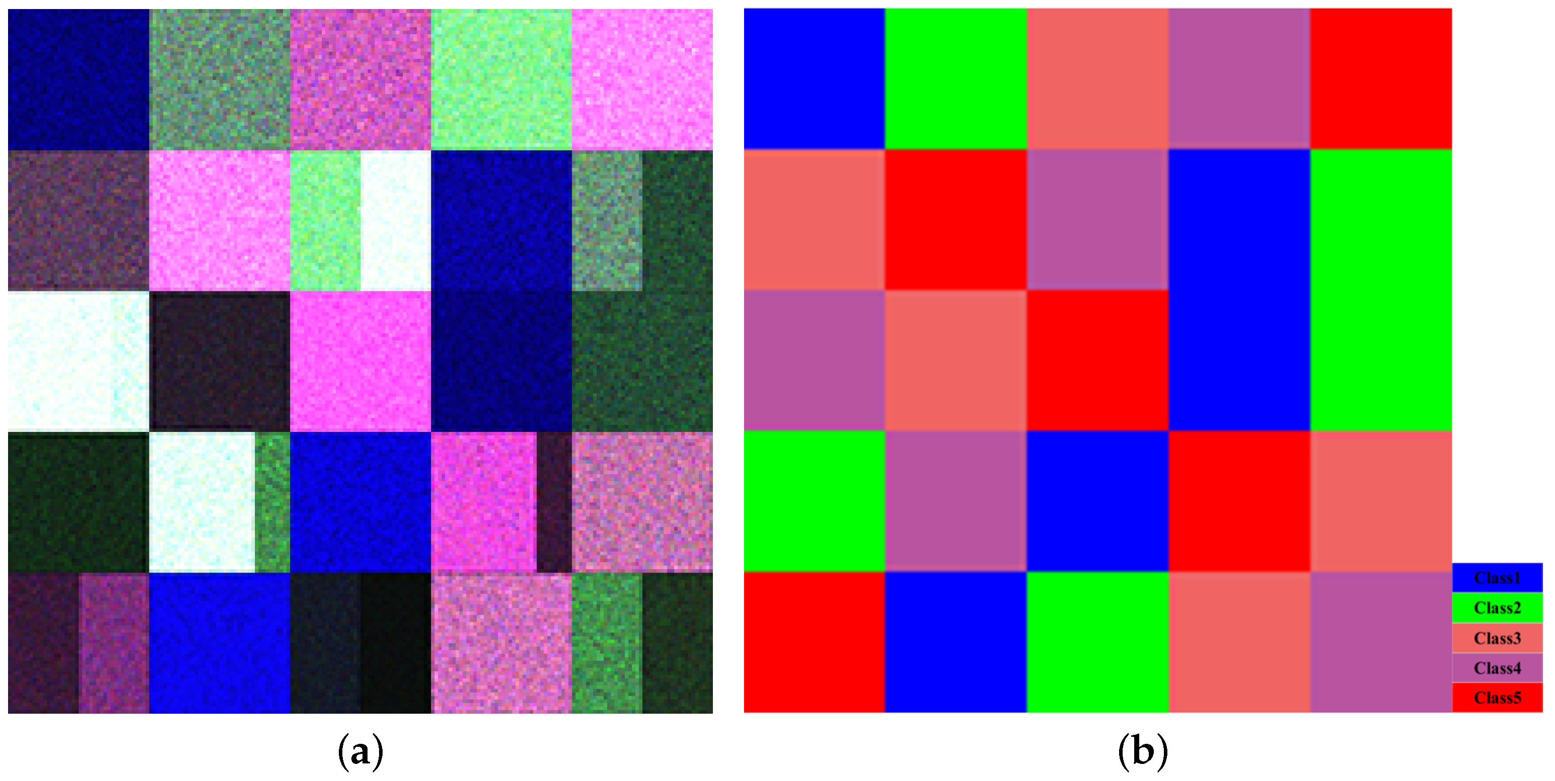
The first dataset is the simulated PolSAR dataset, which is generated utilizing the Monte Carlo method mentioned in [10]. Figure 2 gives the pseudocolor image and the corresponding ground-truth map. The image has $1000\times 1000$ pixels and has five classes. Each class is assumed to consist of five components that follow the Wishart distribution. The relevant parameters are taken from the second PolSAR dataset on the San Francisco area, and the clustering centroids are given in Appendix A.

4.1.2. Real Datasets

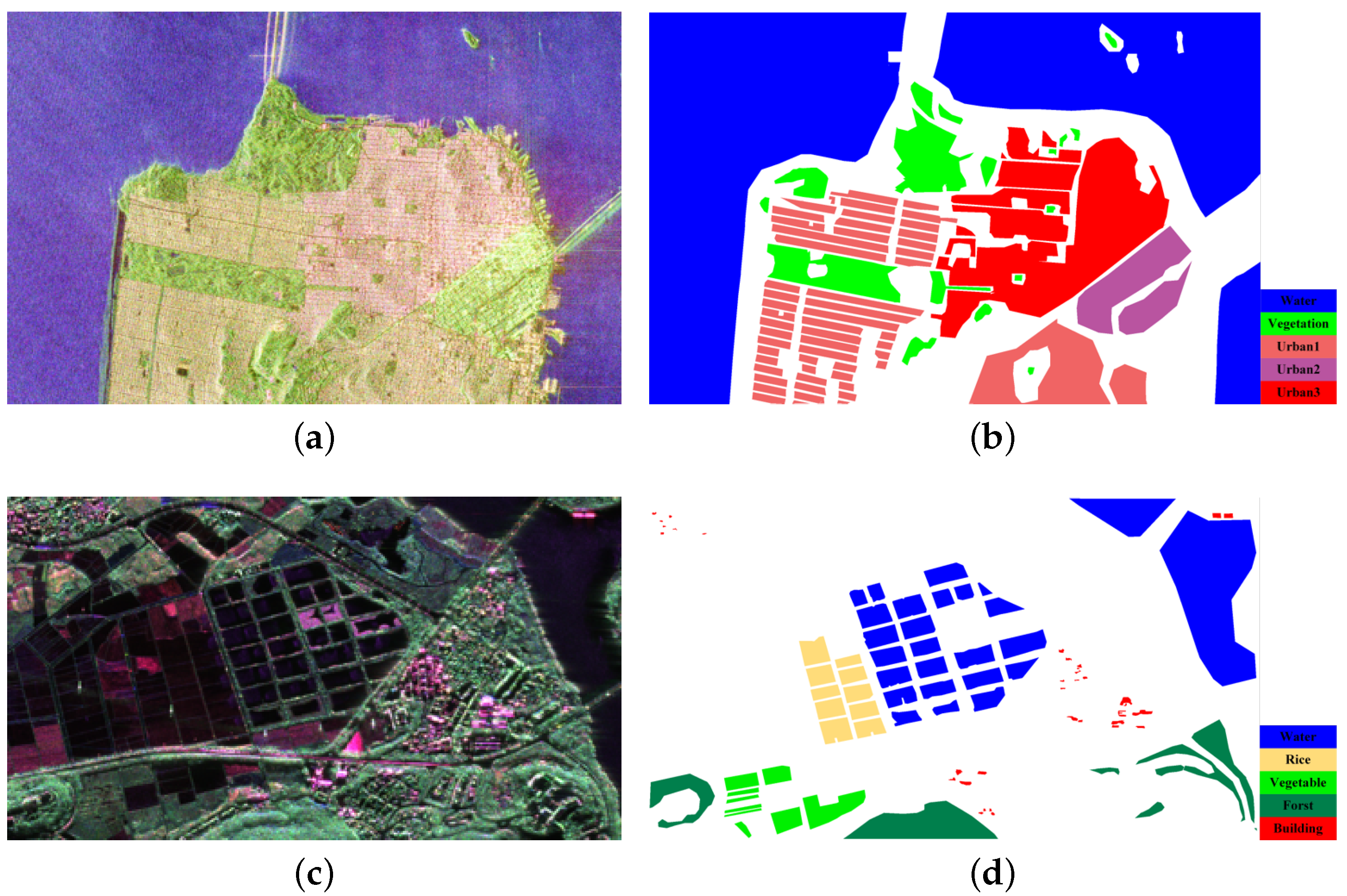
One spaceborne dataset and one airborne dataset are used for the experiments. The second dataset is the fully polarimetric image of the San Francisco region. It was acquired by the C-band GF-3 spaceborne satellite. Figure 3a,b gives the pseudocolor image and the corresponding ground-truth map. The image has $1600\times 2500$ pixels and contains five classes: water, vegetation, and three types of urban areas. The urban areas are classified into three classes based on orientation or density [37]. The third dataset is the L-band fully polarimetric airborne satellite image of Boao town, Hainan province, in China. It was acquired in February 2021 with a 1 m resolution. The image has $1400\times 2500$ pixels in size and has five classes: water, rice, grass, tree, and building. Its pseudocolor image and ground-truth map are shown in Figure 3c,d.

4.2. Performance of the Proposed RWMM

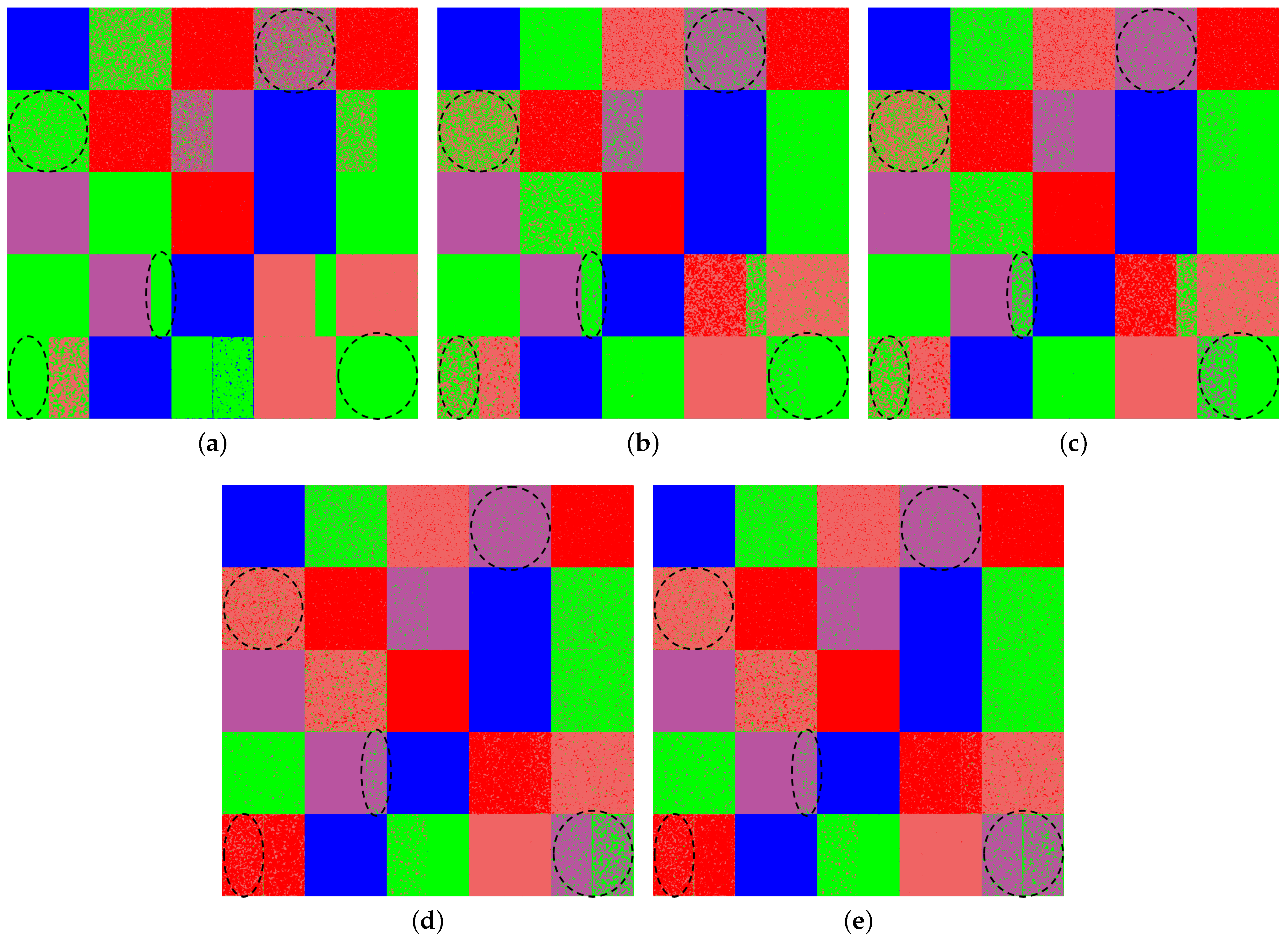
Since RWMM is used to characterize the statistical distribution of the covariance/coherence matrix, it is difficult to visually verify the goodness of fit of RWMM to the distribution of PolSAR data using histograms. According to the foregoing, the ML criterion only depends on the distribution model. Thus, the ML-based classification algorithm is adopted to demonstrate the performance of RWMM in the experiments. Aside from RWMM, the classification results of Wishart, K-Wishart, G, and WMM are also presented for comparison. The simulated PolSAR dataset and two real PolSAR datasets, including the San Francisco and Boao datasets, are taken as examples. Equation (31) is used to obtain classification results after the three datasets have been filtered with a 3 × 3 boxcar filter. In the training step, 1% of the ground-truth data for each class is randomly selected as the training sample, and the remaining data are used as the test sample. Four indicators, including the user’s accuracy (UA), the producer’s accuracy (PA), the overall accuracy (OA), and the Kappa coefficient, are utilized to quantitatively evaluate the classification results. Among them, UA and PA describe the classification results of a specific class, and OA and the Kappa coefficient describe the classification results of the whole PolSAR image. The classification maps of the simulated PolSAR dataset are shown in Figure 4, and

Table 1. The ML-Based Classification Accuracy (%) Comparison of Five Models on the Simulated PolSAR dataset.

Model	Class 1		Class 2		Class 3		Class 4		Class 5		OA	Kappa
	UA	PA	UA	PA	UA	PA	UA	PA	UA	PA
Wishart	99.23	100	51.01	89.73	53.72	42.80	99.97	64.74	73.47	57.96	71.05	0.6381
K-Wishart	100	100	60.44	99.09	74.28	70.71	99.28	71.41	96.57	66.54	81.55	0.7694
G	100	100	63.30	96.74	77.57	78.30	96.75	78.30	96.25	71.00	83.55	0.7944
WMM	100	100	90.95	92.59	91.23	92.38	95.44	93.15	94.50	93.89	94.40	0.9300
RWMM	100	100	92.89	93.93	92.75	92.67	96.22	95.38	95.09	94.95	95.39	0.9423

gives the detailed classification results.

From Table 1, it can be seen that for class 2, the UA of the Wishart model is only 51.01%, which means that 48.99% of the pixels marked as class 2 are from other classes. From Figure 4, it can be seen that some pixels of classes 3–5 are misclassified as class 2 for all five models. This indicates that the scattering mechanism of some pixels in classes 3–5 is similar to class 2. Since the traditional Wishart model cannot accurately characterize the distribution characteristics of class 2, a considerable number of pixels in classes 3–5 are misclassified. Compared with the Wishart model, the UAs of the K-Wishart and G models are 60.44% and 63.30%, respectively, with an improvement of about 10%. This is because the K-Wishart model and G model have a parameter describing texture information, which can model the data more flexibly. It can also be seen from Figure 4b,c that the misclassified pixels are reduced. The UAs of WMM and RWMM is 90.95% and 92.89%, respectively, which is a considerable improvement. This illustrates that the mixture model has higher flexibility than the product model. Overall, RWMM has the highest OA among the five models, which is 95.39%. WMM is followed by 94.40%. The OA of the K-Wishart and G models are 11.84% and 13.84% lower than RWMM. The Wishart model has the lowest OA of 71.05%. This verifies the ability of RWMM to model PolSAR data.

Next, two real datasets are used to illustrate the performance of RWMM. The classification maps from the San Francisco dataset are shown in Figure 5, and

Table 2. The ML-Based Classification Accuracy (%) Comparison of Five Models on the San Francisco Region.

Model	Water		Vegetation		Urban 1		Urban 2		Urban 3		OA	Kappa
	UA	PA	UA	PA	UA	PA	UA	PA	UA	PA
Wishart	99.78	99.86	49.34	92.10	54.67	62.41	79.23	52.88	80.22	43.03	84.00	0.7277
K-Wishart	99.97	99.82	56.68	89.24	63.70	67.99	75.53	61.59	81.61	58.55	87.15	0.7812
G	99.97	99.83	58.38	87.38	65.04	66.97	71.10	66.06	81.03	61.57	87.50	0.7872
WMM	99.97	99.91	65.69	79.35	65.59	62.67	62.49	70.01	73.90	67.96	87.46	0.7862
RWMM	99.97	99.89	67.64	82.25	69.88	63.71	62.62	72.16	76.41	72.32	88.51	0.8042

gives the detailed classification results. In Table 2, the UAs and PAs of the water class are both higher than 99.7% for the five models. This means that a few pixels of the water class are misclassified as urban or vegetation class, and there are also a few pixels belonging to the urban or vegetation classes are misclassified as the water class. Since the scattering mechanism of the water class is quite different from the other classes, the five models can distinguish the water class well. For the vegetation class, the classification map points out that part pixels of three urban classes are misclassified as the vegetation class. The PAs of the vegetation class are higher than the corresponding UAs for all five models, which is consistent with the classification map. Among the five models, RWMM has the highest UA of 67.64%, while PA is also at a relatively high value of 82.25%. For the three urban classes, due to the similarity of the scattering mechanism, the classification accuracy UA and PA are not very high. Compared with other models, RWMM still has a better classification result. The Wishart model achieves an OA of 84.00%, which is the worst classification performance. Compared with the Wishart model, the OAs of K-Wishart, G, WMM, and RWMM are improved by 3.15%, 3.50%, 3.46%, and 4.51%, respectively. Overall, the OAs of the product model and the mixture model do not improve much in the San Francisco region. However, the proposed RWMM still has the highest overall classification accuracy and Kappa coefficient. This verifies the ability of RWMM to model PolSAR data again.

Figure 6 gives the classification maps of the Boao dataset, and the detailed results are shown in

Table 3. The ML-Based Classification Accuracy (%) Comparison of Five Models on the Boao Region.

Model	Water		Vegetation		Urban 1		Urban 2		Urban 3		OA	Kappa
	UA	PA	UA	PA	UA	PA	UA	PA	UA	PA
Wishart	98.44	70.92	39.41	91.92	55.04	91.11	94.87	76.60	88.61	91.84	76.35	0.6489
K-Wishart	98.38	80.15	48.78	92.13	59.34	89.67	94.84	79.43	92.73	95.78	82.35	0.7268
G	98.40	78.51	46.38	92.75	61.17	88.38	94.28	80.58	95.77	94.41	81.55	0.7163
WMM	98.36	91.45	69.32	92.46	61.78	84.63	92.99	80.56	92.91	97.09	88.93	0.8192
RWMM	98.42	92.10	70.79	92.54	64.64	88.60	94.86	81.49	90.91	98.05	89.84	0.8337

. In Table 3, the UAs of the water class are higher than the corresponding PAs for all five models. This indicates that some pixels of the water class were wrongly classified into other classes. The PAs of the rice class are higher than the corresponding UAs for all five models, indicating that part pixels of other classes were wrongly classified into the rice class. Combined with the classification map, it can be seen that the five models have some difficulty in distinguishing between the water and rice classes. After an on-the-spot investigation, we found that the rice fields had just been planted, so the rice is in the early stage of growth and is very sparsely distributed in the paddy field. L-band electromagnetic waves can easily penetrate the stems and leaves of rice to the water’s surface [38]. Therefore, rice and water classes are not easy to distinguish for L-band PolSAR data. Compared with other models, RWMM can achieve a better balance for UA and PA. Overall, the proposed RWMM still has the highest OA, which is 89.84%, followed by WMM with 88.93%. The OAs of the two product models: K-Wishart and G models, are 82.35% and 81.55%, respectively. The Wishart model has the lowest classification accuracy among the five models, and its OA is only 76.35%. The OAs of the two mixture models are more than 12% higher than the Wishart model and 7% higher than the two product models, which is a considerable improvement compared with the classification results on the GF-3 data. A possible reason is that the resolutions of the two datasets are different. Compared with the 8-m resolution of the GF-3 satellite, the airborne satellite has a resolution of 1 m. In high-resolution PolSAR images, the degree of heterogeneity of the scene increases. This makes the Wishart model and the two product models unable to characterize the distribution of PolSAR data well.

From the classification results of the simulated PolSAR dataset and the two real PolSAR datasets, it can be seen that RWMM has the highest overall classification accuracy among the five models. For the ML-based classification algorithms, the results only depend on statistical models. Therefore, the classification results verify the effectiveness of RWMM in modeling PolSAR data.

4.3. Classification Results and Analysis of the Proposed RWMM-MRF Algorithm

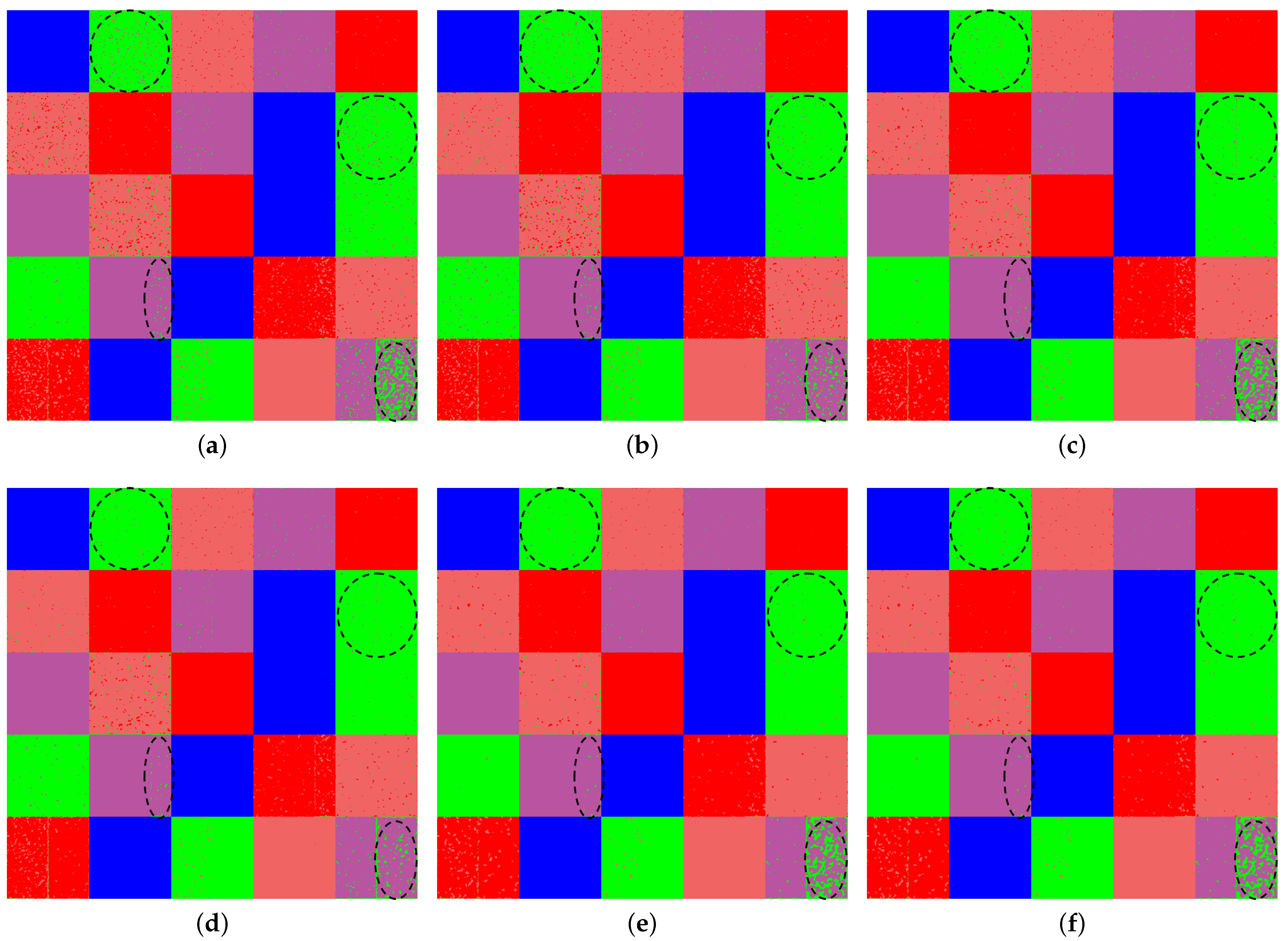
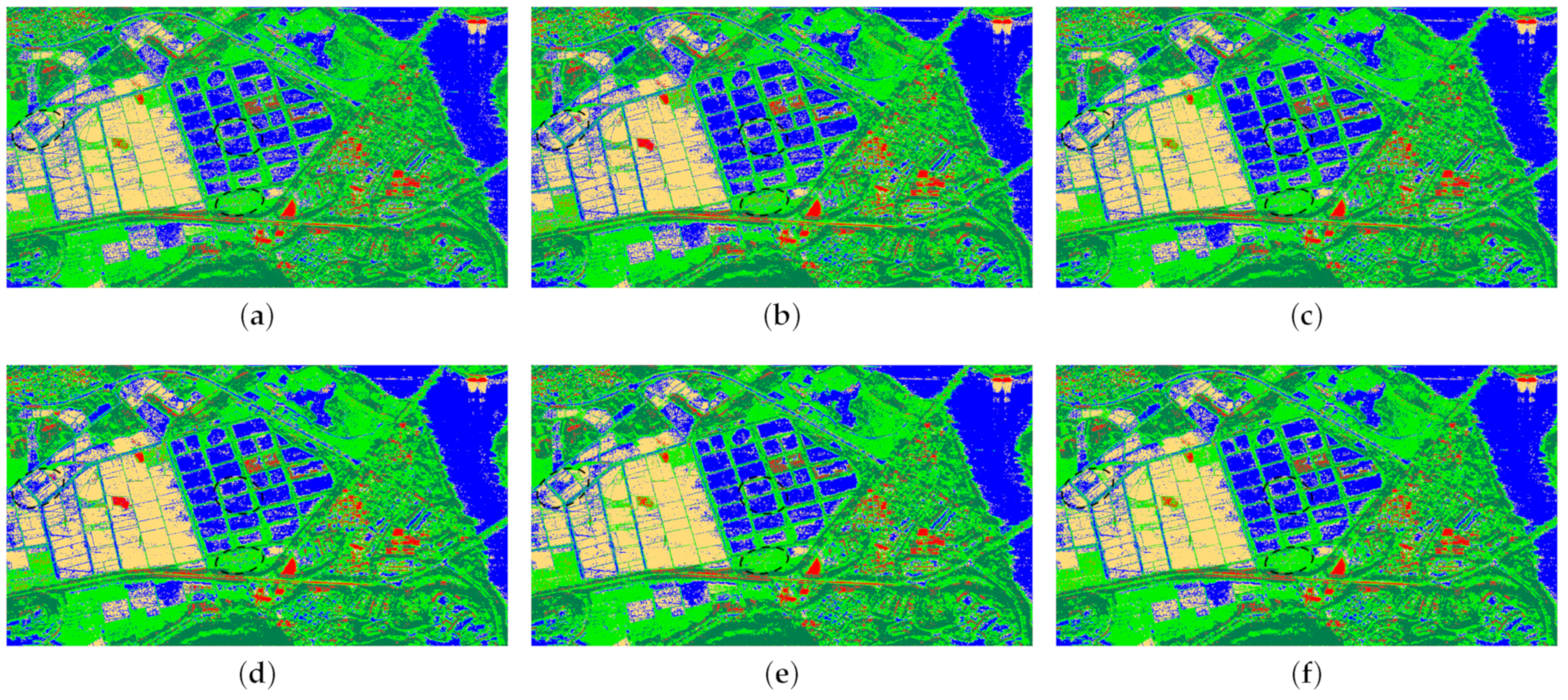
Here, WMM and RWMM are chosen as the likelihood terms combined with MRF for the PolSAR classification. To illustrate the performance of the new selection criterion, two different criteria are additionally adopted. First, a fixed neighborhood, which is ${\eta }_1$ in Figure 1, is used. The corresponding classification algorithms are named WMM-MRF and RWMM-MRF. Then, the selection criterion (22) is used, and WMM-MRFs and RWMM-MRFs are the corresponding classification algorithms. WMM-MRFt and RWMM-MRFt are the classification algorithms that indicate the neighborhood is selected by the proposed selection criterion (25). The simulated PolSAR dataset and two real PolSAR datasets, including the San Francisco and Boao datasets, are taken as examples. The three PolSAR datasets are filtered by a $3\times 3$ boxcar filter. Based on the algorithms mentioned above, the classification maps of the simulated PolSAR dataset are shown in Figure 7.

Table 4. Classification Accuracy (%) Of Six Different Algorithms on the simulated PolSAR dataset.

Model	Water		Vegetation		Urban 1		Urban 2		Urban 3		OA	Kappa
	UA	PA	UA	PA	UA	PA	UA	PA	UA	PA
WMM-MRF	100	100	93.91	97.59	95.18	96.56	98.60	94.76	97.51	96.08	97.00	0.9624
RWMM-MRF	100	100	96.15	98.23	96.29	96.70	99.00	97.26	97.80	96.98	97.83	0.9729
WMM-MRFs	100	100	94.94	98.85	96.49	98.09	99.35	95.50	98.74	96.87	97.86	0.9733
RWMM-MRFs	100	100	97.03	99.16	97.31	97.97	99.55	97.89	98.78	97.60	98.52	0.9815
WMM-MRFt	100	100	95.50	99.36	97.74	98.90	99.71	95.75	99.26	98.01	98.40	0.9801
RWMM-MRFt	100	100	97.68	99.49	98.19	98.61	99.76	98.27	99.18	98.39	98.95	0.9869

gives the corresponding classification results.

Compared with the classification result of WMM in Table 1, the OA of WMM-MRF, WMM-MRFs, and WMM-MRFt are improved by 2.60%, 3.46%, and 4%, respectively. Similarly, compared with the OA of RWMM in Table 1, the RWMM-MRF, RWMM-MRFs, and RWMM-MRFt are improved by 2.44%, 3.13%, and 3.56%, respectively. Therefore, it can be proven that MRF-based algorithms can further improve classification accuracy. From Table 4, it can be noticed that the RWMM-MRFt has the highest overall classification accuracy among the three classification algorithms of RWMM combined with MRF. The RWMM-MRFs follow behind, and the RWMM-MRF has the worst classification result. For WMM, three classification algorithms have similar results. This demonstrates that the MRF-based classification algorithm with an AN system has better performance than the one with a fixed neighborhood, and proposed criterion (25) is superior to criterion (22). The classification results validate the theoretical analysis that the proposed criterion makes effective use of PolSAR scattering information. However, criterion (22) only uses the span information. Moreover, RWMM-MRFt still has the highest OA and Kappa coefficient among the six mixture model-based MRF classification algorithms, which are 98.95% and 0.9869. The OA of the proposed supervised classification algorithm (i.e., RWMM-MRFt) is improved by about 5% compared with WMM, improved by about 2% compared with WMM-MRF, and improved by about 1% compared with WMM-MRFs. The classification result verifies the effectiveness of the proposed classification algorithm.

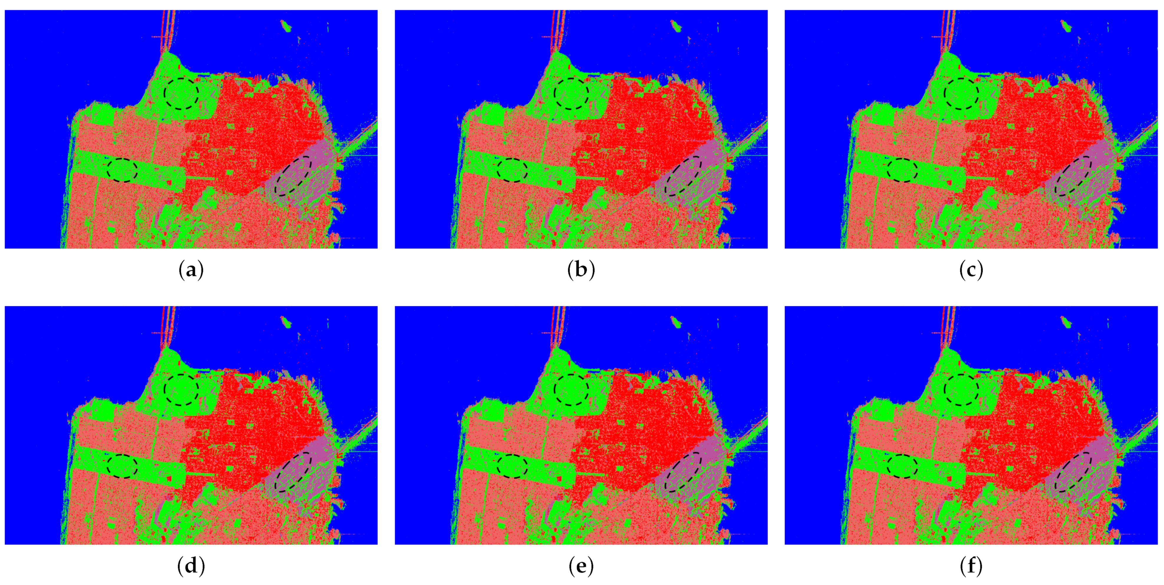
Next, two real datasets, including the San Francisco and Boao datasets, are used to illustrate the classification performance of the proposed RWMM-MRFt algorithm. The classification maps for the San Francisco dataset are shown in Figure 8, and

Table 5. Classification Accuracy (%) Of Six Different Algorithms on the San Francisco region.

Model	Water		Vegetation		Urban 1		Urban 2		Urban 3		OA	Kappa
	UA	PA	UA	PA	UA	PA	UA	PA	UA	PA
WMM-MRF	99.98	99.94	70.89	85.51	72.45	70.32	69.97	73.66	79.57	73.07	89.87	0.8271
RWMM-MRF	99.98	99.94	72.44	86.38	76.01	70.35	69.43	75.79	80.65	77.34	90.63	0.8401
WMM-MRFs	99.98	99.95	72.32	90.16	74.24	74.56	75.04	74.26	82.86	73.17	90.82	0.8434
RWMM-MRFs	99.99	99.94	73.69	91.21	78.28	76.50	75.54	76.49	85.33	77.48	91.88	0.8614
WMM-MRFt	99.98	99.95	77.30	91.65	79.78	80.03	78.88	78.13	86.36	78.83	92.67	0.8748
RWMM-MRFt	99.99	99.95	79.99	92.52	85.57	82.24	80.09	80.72	88.34	85.08	94.05	0.8984

gives the detailed classification results. From Table 5, it can be seen that the proposed RWMM-MRFt has the highest OA of 94.05%. The OA of RWMM-MRFt is 2.17% higher than RWMM-MRFs. This proves that the proposed selection criterion (25) is more favorable for the center pixel to select the appropriate neighborhood. However, the OA of RWMM-MRFt is only 0.43% higher than that of RWMM-MRFs on the simulated PolSAR dataset. One possible reason is that the number of pixels in the boundary locations in San Francisco is much larger than the simulated scene, and the new selection criterion can more accurately select the most suitable neighborhood for these pixels. Similar results can also be seen from the classification performance of the WMM-MRFs and WMM-MRFt algorithms. It can be seen from Table 5 that no matter what neighborhood selection criterion is used in MRF, the OA of RWMM combined with MRF is always higher than the corresponding WMM combined with MRF. This demonstrates that RWMM performs better than WMM in acting as the likelihood term under the MAP classification framework. Overall, the OA of the proposed classification algorithm is improved by about 7% compared with WMM, improved by about 4% compared with WMM-MRF, and improved by about 3% compared with WMM-MRFs. The classification results verify the effectiveness of the proposed classification algorithm again.

The classification maps of the Boao dataset are shown in Figure 9. The quantitative results are given in

Table 6. Classification Accuracy (%) of Six Different Algorithms on the Boao region.

Model	Water		Vegetation		Urban 1		Urban 2		Urban 3		OA	Kappa
	UA	PA	UA	PA	UA	PA	UA	PA	UA	PA
WMM-MRF	98.83	93.34	75.33	94.38	65.75	88.59	94.78	83.25	94.35	97.42	91.13	0.8540
RWMM-MRF	98.87	93.97	76.87	94.52	66.87	90.58	95.74	83.20	93.14	98.73	91.68	0.8628
WMM-MRFs	99.03	94.34	78.55	95.25	67.09	91.76	96.19	83.63	95.51	97.57	92.15	0.8704
RWMM-MRFs	99.07	95.27	81.32	95.44	67.61	93.01	96.85	83.34	95.55	98.79	92.78	0.8804
WMM-MRFt	99.16	94.85	80.48	95.82	69.19	92.51	96.55	85.22	95.16	97.61	92.89	0.8824
RWMM-MRFt	99.26	95.91	83.99	96.30	69.28	93.62	97.14	84.64	94.97	99.34	93.58	0.8933

.

Compared with the classification results of WMM in Table 3, the OAs of WMM-MRF, WMM-MRFs, and WMM-MRFt are improved by 3.67%, 4.69%, and 5.43%, respectively. Similarly, compared with the classification results of RWMM in Table 3, the OAs of RWMM-MRF, RWMM-MRFs, and RWMM-MRFt are improved by 3.17%, 4.27%, and 5.07%, respectively. This once again proves the validity of the proposed selection criterion for the AN system, and proposed criterion (25) is superior to criterion (22). Moreover, RWMM-MRFt has the highest OA and Kappa coefficient among the classification algorithms for the Boao dataset, which are 93.58% and 0.8933. It can be seen from Figure 9 that the RWMM-MRFt classification map has a strong anti-noise ability and obtains a smoother homogeneous area, which again verifies the effectiveness of the proposed classification algorithm.

Overall, the OA of the proposed supervised classification algorithm is improved by about 5–7% compared with WMM, improved by about 2–4% compared with WMM-MRF, and improved by about 1–3% compared with WMM-MRFs. Both simulated and real PolSAR data demonstrate the superiority of the proposed supervised classification algorithm.

5. Discussion

In this paper, RWMM is used for supervised classification. For supervised classification, RWMM is used to characterize the statistical distribution of data belonging to a single class. The number of mixture components represents the number of subclasses in a single class. As K increases, that is, a single class is divided into more and more subclasses, the modeling accuracy of RWMM on the data gradually increases first and then tends to stabilize. In [18], the overall classification accuracy generally increases when K is gradually increased to 10 and only slightly increases when K is further increased. This is consistent with the theoretical analysis. We also analyzed the influence of the number of mixture components based on the simulated and real PolSAR data. The results show that $K=10$ is sufficient for RWMM to model the PolSAR data accurately. When K continues to increase, the improvement of the overall classification accuracy is very limited. Take the Boao region as an example; when K = 1, 3, 5, and 10, the OA of RWMM is 76.40%, 88.78%, 89.17%, and 89.84%, respectively. However, when K = 12, 15, and 20, the OA of RWMM is 89.84%, 89.89%, and 90.03%, respectively. Therefore, K = 10 is set for the proposed algorithm.

In fact, RWMM can also be used for unsupervised classifications. For unsupervised classifications, RWMM is used to characterize the statistical distribution of the whole PolSAR image, where the number of mixture components K represents the number of classes in the scene. When K is set too small, data of different classes will be classified into one class, and when K is too large, data belonging to one class will be split. Therefore, an adaptive method for determining the number of mixture components is necessary for unsupervised classification. In [39], a mixture component is preset at initialization, and then every few iterations, the current components are split and merged. A goodness-of-fit testing strategy is employed to control for splitting and merging. In this paper, K is set to a large value at initialization, and a merging strategy can be performed in the last step of parameter estimation. This is to avoid splitting components. Compared to the method in [39], although this method may be difficult to precisely determine the number of classes in the scene, it avoids re-estimating the parameters at each split. It should be emphasized that for supervised classification, it is not necessary to accurately estimate the number of mixture components.

6. Conclusions

This paper first proposes a new mixture Wishart model named RWMM. Compared with WMM, RWMM does not introduce new parameters, so the mathematical complexity of the statistical model does not increase. RWMM further improves the goodness of fi,t the model to the distribution of PolSAR data by relaxing the number of looks parameters. The EM algorithm is utilized to estimate parameters through an iterative process. The ML-based classification results of simulated and real PolSAR datasets show that RWMM has the highest overall classification accuracy and Kappa coefficient. It demonstrates that RWMM has greater flexibility and effectiveness than the Wishart, K-Wishart, G, and WMM models in modeling PolSAR data. Then, MRF is used to improve the classification results by fusing the spatial information in the PolSAR images. In the MRF process, an AN system is adopted, and a new criterion is proposed to further improve the overall classification accuracy. The new criterion can make more effective use of the PolSAR scattering information than the selection criterion based on span. Regardless of whether the statistical model used is WMM or RWMM, the classification results indicate that the proposed criterion based on the complex-kind HLT statistic can find a more suitable neighborhood than the criterion based on span.

Based on RWMM and the new selection criterion for the AN system, a new supervised classification algorithm named RWMM-MRFt is proposed. The proposed algorithm classifies PolSAR images according to the likelihood probability obtained by RWMM and the prior probability obtained by MRF. The classification results of the simulated and two real PolSAR datasets, including the San Francisco and Boao datasets, have shown that RWMM-MRFt has the highest overall classification accuracy and Kappa coefficient among the mixture model-based MRF classification algorithms. Overall, the classification accuracy of the proposed algorithm is improved by about 5–7% compared with WMM, improved by about 2–4% compared with WMM-MRF, and improved by about 1–3% compared with WMM-MRFs. The results demonstrate the superiority of the RWMM-MRFt algorithm in PolSAR data classification. The proposed algorithm belongs to the conventional classification algorithm, and the classification accuracy may not be as high as that of machine learning and deep learning algorithms. However, it has simple expressions and clear physical meanings. The AN system in the proposed algorithm has only five simple neighborhoods, which may not fully represent the shape of the regional boundary. In future work, more neighborhoods could be added to the AN system to further improve the classification accuracy.

References

1. Qi, Z.; Yeh, A.G.O.; Li, X.; Lin, Z. A novel algorithm for land use and land cover classification using RADARSAT-2 polarimetric SAR data. Remote Sens. Environ. 2012, 118, 21–39. [Google Scholar] [CrossRef]
2. Liu, C.; Gierull, C.H. A new application for PolSAR imagery in the field of moving target indication/ship detection. IEEE Trans. Geosci. Remote Sens. 2007, 45, 3426–3436. [Google Scholar] [CrossRef]
3. Yonezawa, C.; Watanabe, M.; Saito, G. Polarimetric decomposition analysis of ALOS PALSAR observation data before and after a landslide event. Remote Sens. 2012, 4, 2314–2328. [Google Scholar] [CrossRef] [Green Version]
4. Chen, S.W.; Sato, M. Tsunami damage investigation of built-up areas using multitemporal spaceborne full polarimetric SAR images. IEEE Trans. Geosci. Remote Sens. 2012, 51, 1985–1997. [Google Scholar] [CrossRef]
5. Van Zyl, J.; Carande, R.; Lou, Y.; Miller, T.; Wheeler, K. The NASA/JPL three-frequency polarimetric AIRSAR system. In Proceedings of the IGARSS’92 International Geoscience and Remote Sensing Symposium, Houston, TX, USA, 26–29 May 1992; IEEE: Piscataway, NJ, USA, 1992; Volume 1, pp. 649–651. [Google Scholar]
6. Morena, L.; James, K.; Beck, J. An introduction to the RADARSAT-2 mission. Can. J. Remote Sens. 2004, 30, 221–234. [Google Scholar] [CrossRef]
7. Sun, J.; Yu, W.; Deng, Y. The SAR payload design and performance for the GF-3 mission. Sensors 2017, 17, 2419. [Google Scholar] [CrossRef] [Green Version]
8. Shang, R.; He, J.; Wang, J.; Xu, K.; Jiao, L.; Stolkin, R. Dense connection and depthwise separable convolution based CNN for polarimetric SAR image classification. Knowl.-Based Syst. 2020, 194, 105542. [Google Scholar] [CrossRef]
9. Shang, R.; Wang, G.; Okoth, M.A.; Jiao, L. Complex-valued convolutional autoencoder and spatial pixel-squares refinement for polarimetric SAR image classification. Remote Sens. 2019, 11, 522. [Google Scholar] [CrossRef] [Green Version]
10. Lee, J.S.; Pottier, E. Polarimetric Radar Imaging: From Basics to Applications; CRC Press: Boca Raton, FL, USA, 2017. [Google Scholar]
11. Kong, J.; Swartz, A.; Yueh, H.; Novak, L.; Shin, R. Identification of terrain cover using the optimum polarimetric classifier. J. Electromagn. Waves Appl. 1988, 2, 171–194. [Google Scholar]
12. Lee, J.S.; Grunes, M.R.; Kwok, R. Classification of multi-look polarimetric SAR imagery based on complex Wishart distribution. Int. J. Remote Sens. 1994, 15, 2299–2311. [Google Scholar] [CrossRef]
13. Dong, H.; Xu, X.; Sui, H.; Xu, F.; Liu, J. Copula-based joint statistical model for polarimetric features and its application in PolSAR image classification. IEEE Trans. Geosci. Remote Sens. 2017, 55, 5777–5789. [Google Scholar] [CrossRef]
14. Lopes, A.; Séry, F. Optimal speckle reduction for the product model in multilook polarimetric SAR imagery and the Wishart distribution. IEEE Trans. Geosci. Remote Sens. 1997, 35, 632–647. [Google Scholar] [CrossRef]
15. Lee, J.; Schuler, D.; Lang, R.; Ranson, K. K-distribution for multi-look processed polarimetric SAR imagery. In Proceedings of the IGARSS’94-1994 IEEE International Geoscience and Remote Sensing Symposium, Pasadena, CA, USA, 8–12 August 1994; IEEE: Piscataway, NJ, USA, 1994; Volume 4, pp. 2179–2181. [Google Scholar]
16. Freitas, C.C.; Frery, A.C.; Correia, A.H. The polarimetric G distribution for SAR data analysis. Environ. Off. J. Int. Environ. Soc. 2005, 16, 13–31. [Google Scholar] [CrossRef]
17. Harant, O.; Bombrun, L.; Gay, M.; Fallourd, R.; Trouvé, E.; Tupin, F. Segmentation and classification of polarimetric SAR data based on the KummerU distribution. In Proceedings of the POLinSAR 2009-4th International Workshop on Science and Applications of SAR Polarimetry and Polarimetric Interferometry, Frascati, Italy, 26–30 January 2009; p. 6. [Google Scholar]
18. Gao, W.; Yang, J.; Ma, W. Land cover classification for polarimetric SAR images based on mixture models. Remote Sens. 2014, 6, 3770–3790. [Google Scholar] [CrossRef] [Green Version]
19. Kersten, P.R.; Lee, J.S.; Ainsworth, T.L. Unsupervised classification of polarimetric synthetic aperture radar images using fuzzy clustering and EM clustering. IEEE Trans. Geosci. Remote Sens. 2005, 43, 519–527. [Google Scholar] [CrossRef]
20. Anfinsen, S.N.; Eltoft, T.; Doulgeris, A.P. A relaxed Wishart model for polarimetric SAR data. In Proceedings of the PolInSAR, Frascati, Italy, 26–30 January 2009; Citeseer: Pennsylvania, PA, USA, 2009; p. 42. [Google Scholar]
21. Li, S.Z. Markov Random Field Modeling in Image Analysis; Springer Science & Business Media: Berlin/Heidelberg, Germany, 2009. [Google Scholar]
22. Yamazaki, T.; Gingras, D. Image classification using spectral and spatial information based on MRF models. IEEE Trans. Image Process. 1995, 4, 1333–1339. [Google Scholar] [CrossRef] [PubMed] [Green Version]
23. Li, W.; Prasad, S.; Fowler, J.E. Hyperspectral image classification using Gaussian mixture models and Markov random fields. IEEE Geosci. Remote Sens. Lett. 2013, 11, 153–157. [Google Scholar] [CrossRef] [Green Version]
24. Wu, Y.; Ji, K.; Yu, W.; Su, Y. Region-based classification of polarimetric SAR images using Wishart MRF. IEEE Geosci. Remote Sens. Lett. 2008, 5, 668–672. [Google Scholar] [CrossRef]
25. Smits, P.C.; Dellepiane, S.G. Synthetic aperture radar image segmentation by a detail preserving Markov random field approach. IEEE Trans. Geosci. Remote Sens. 1997, 35, 844–857. [Google Scholar] [CrossRef]
26. Murtagh, F.; Contreras, P.; Starck, J.L. Scale-based gaussian coverings: Combining intra and inter mixture models in image segmentation. Entropy 2009, 11, 513–528. [Google Scholar] [CrossRef]
27. Chen, J.; Wang, Y.; Wu, H. A coded aperture compressive imaging array and its visual detection and tracking algorithms for surveillance systems. Sensors 2012, 12, 14397–14415. [Google Scholar] [CrossRef] [PubMed]
28. Oliver, C.; Quegan, S. Understanding Synthetic Aperture Radar Images; SciTech Publishing: Southampton, UK, 2004. [Google Scholar]
29. Anfinsen, S.N.; Doulgeris, A.P.; Eltoft, T. Estimation of the equivalent number of looks in polarimetric synthetic aperture radar imagery. IEEE Trans. Geosci. Remote Sens. 2009, 47, 3795–3809. [Google Scholar] [CrossRef]
30. McLachlan, G.J.; Krishnan, T. The EM Algorithm and Extensions; John Wiley & Sons: Hoboken, NJ, USA, 2007. [Google Scholar]
31. Kulis, B.; Sustik, M.A.; Dhillon, I.S. Low-Rank Kernel Learning with Bregman Matrix Divergences. J. Mach. Learn. Res. 2009, 10. [Google Scholar]
32. Geman, S.; Geman, D. Stochastic relaxation, Gibbs distributions, and the Bayesian restoration of images. IEEE Trans. Pattern Anal. Mach. Intell. 1984, PAMI-6, 721–741. [Google Scholar] [CrossRef] [PubMed]
33. Rignot, E.; Chellappa, R. Segmentation of synthetic-aperture-radar complex data. JOSA A 1991, 8, 1499–1509. [Google Scholar] [CrossRef]
34. Cao, F.; Hong, W.; Wu, Y.; Pottier, E. An Unsupervised Segmentation With an Adaptive Number of Clusters Using the SPAN/H/α/A Space and the Complex Wishart Clustering for Fully Polarimetric SAR Data Analysis. IEEE Trans. Geosci. Remote Sens. 2007, 45, 3454–3467. [Google Scholar] [CrossRef]
35. Akbari, V.; Anfinsen, S.N.; Doulgeris, A.P.; Eltoft, T.; Moser, G.; Serpico, S.B. Polarimetric SAR change detection with the complex Hotelling–Lawley trace statistic. IEEE Trans. Geosci. Remote Sens. 2016, 54, 3953–3966. [Google Scholar] [CrossRef] [Green Version]
36. Anfinsen, S.N.; Eltoft, T. Application of the matrix-variate Mellin transform to analysis of polarimetric radar images. IEEE Trans. Geosci. Remote Sens. 2011, 49, 2281–2295. [Google Scholar] [CrossRef]
37. Liu, X.; Jiao, L.; Tang, X.; Sun, Q.; Zhang, D. Polarimetric convolutional network for PolSAR image classification. IEEE Trans. Geosci. Remote Sens. 2018, 57, 3040–3054. [Google Scholar] [CrossRef] [Green Version]
38. Wang, C.; Wu, J.; Zhang, Y.; Pan, G.; Qi, J.; Salas, W.A. Characterizing L-band scattering of paddy rice in southeast China with radiative transfer model and multitemporal ALOS/PALSAR imagery. IEEE Trans. Geosci. Remote Sens. 2009, 47, 988–998. [Google Scholar] [CrossRef]
39. Doulgeris, A.P.; Anfinsen, S.N.; Eltoft, T. Automated non-Gaussian clustering of polarimetric synthetic aperture radar images. IEEE Trans. Geosci. Remote Sens. 2011, 49, 3665–3676. [Google Scholar] [CrossRef]
Figure 1. Five neighborhoods in the AN system.
Remotesensing 14 05506 g001
Figure 2. The simulated PolSAR images and the corresponding ground-truth maps. (a) Pseudocolor image of the simulated PolSAR dataset. (b) Ground-truth map of (a) (5 classes).
Remotesensing 14 05506 g002
Figure 3. The real PolSAR images and the corresponding ground-truth maps. (a) Pseudocolor image of San Francisco region. (b) Ground-truth map of (a) (5 classes). (c) Pseudocolor image of Boao region. (d) Ground-truth map of (c) (5 classes).
Remotesensing 14 05506 g003
Figure 4. The ML-based classification maps of five models on the simulated PolSAR dataset. (a) Wishart. (b) K-Wishart. (c) G. (d) WMM. (e) RWMM.
Remotesensing 14 05506 g004
Figure 5. The ML-based classification maps of five models on the San Francisco region. (a) Wishart. (b) K-Wishart. (c) G. (d) WMM. (e) RWMM.
Remotesensing 14 05506 g005
Figure 6. The ML-based classification maps of five models on the Boao region. (a) Wishart. (b) K-Wishart. (c) G. (d) WMM. (e) RWMM.
Remotesensing 14 05506 g006
Figure 7. Classification maps of six algorithms on the simulated PolSAR dataset. (a) WMM-MRF. (b) RWMM-MRF. (c) WMM-MRFs. (d) RWMM-MRFs. (e) WMM-MRFt. (f) RWMM-MRFt.
Remotesensing 14 05506 g007
Figure 8. Classification maps of six algorithms on the San Francisco region. (a) WMM-MRF. (b) RWMM-MRF. (c) WMM-MRFs. (d) RWMM-MRFs. (e) WMM-MRFt. (f) RWMM-MRFt.
Remotesensing 14 05506 g008
Figure 9. Classification maps of six algorithms on the Boao region. (a) WMM-MRF. (b) RWMM-MRF. (c) WMM-MRFs. (d) RWMM-MRFs. (e) WMM-MRFt. (f) RWMM-MRFt.
Remotesensing 14 05506 g009