Abstract
An object detection pipeline comprises a camera that captures the scene and an object detector that processes these images. The quality of the images directly affects the performance of the object detector. Current works focus on independently improving the image quality or object detection models but neglect the importance of joint optimization of the two subsystems. This paper aims to tune the detection throughput and accuracy of existing object detectors in the remote sensing scenario by optimizing the input images tailored to the object detector. We empirically analyze the influence of two selected camera calibration parameters (camera distortion correction and gamma correction) and five image parameters (quantization, compression, resolution, color model, and additional channels) for these applications. For our experiments, we utilize three Unmanned Aerial Vehicle (UAV) data sets from different domains and a mixture of large and small state-of-the-art object detector models to provide an extensive evaluation of the influence of the pipeline parameters. Finally, we realize an object detection pipeline prototype on an embedded platform for a UAV and give a best practice recommendation for building object detection pipelines based on our findings. We show that not all parameters have an equal impact on detection accuracy and data throughput. Using a suitable compromise between parameters, we can achieve higher detection accuracy for lightweight object detection models while keeping the same data throughput.
1. Introduction
Micro-Aerial Vehicles (MAVs) and Unmanned Aerial Vehicles (UAVs) can support surveillance tasks in many applications. Examples are traffic surveillance in urban environments [1], or search and rescue missions in maritime environments [2], or the much more general task of remote sensing object detection [3]. For these tasks, object detection pipelines are used to support the human operator and simplify the task. The camera system and the object detector are two key components of these detection pipelines. The interaction of these components, normally based on image data, is crucial for the performance of the whole pipeline.
In most projects, the configuration of these components has to be conducted at an early stage. A recording of a necessary data set should be already done with the final camera system. Moreover, the camera system should be optimized based on an existing data set. This situation leads to a chicken-and-egg problem.
The emerging trend toward smart cameras, combining the camera and the computing unit, confirms the need for classification and detection pipelines in embedded systems. The lack of flexibility and the high price of these closed systems remain significant drawbacks and prevent their usage in many research projects or prototyping.
In this work, we want to analyze selected camera parameters and measure their impact on the performance of the detection pipeline in the remote sensing application. We have chosen seven parameters (quantization, compression, color model, resolution, multispectral recordings, and camera calibration), which are easy to adjust for many systems or worth considering. By varying these parameters separately, their effect on the detection performance can be analyzed. With optimized parameters, we assume the pipeline is used more efficiently. This should allow, e.g., a higher throughput of the detection pipeline. By finding the sweet spots and analyzing the impact of the seven camera parameters, we want to provide recommendations for further projects. The experiments are performed in a desktop and an embedded environment, as both are relevant for remote sensing. An embedded object detection pipeline mounted on a UAV using the provided recommendations should prove the usability of the results.
Related Work
The image processing pipeline significantly impacts the performance of object detectors. Many parameters influence this pipeline. However, there is still a lack of impact analysis for UAV-based systems. Yahyanejad et al. have measured the impact of lens distortion correction for thermal images acquired by UAVs [4]. However, their results are only helpful for a thermal camera system.
Other existing camera parameter evaluations are mostly based on the autonomous driving scenario [5,6,7,8,9,10]. The findings of the autonomous driving experiments cannot be directly applied to the remote sensing use case. The scene is often homogenous for autonomous driving, and the object sizes differ only slightly. Further, the distance to the objects is often only a couple of meters. For remote sensing recordings, the distance to the scene is often over 30 m [2], resulting in tiny objects. Depending on the camera angle, the images can vary strongly. Because of these differences, the results of one scenario are not completely valid in the other but can give the first sign.
Balsinski et al. proposed a rendering framework to evaluate camera architectures in simple autonomous driving scenarios [5]. Secci et al. evaluated camera failures in the autonomous driving application [10]. Besides these, the works of Liu et al. [7], Carlson et al. [6] and Saad et al. [9] showed the still existing gap between synthetic and real-world data. Thus, our experiments are based entirely on real-world recordings.
Buckler et al. analyzed the image pipeline regarding performance and energy consumption [11]. In contrast to their work, we close the gap for a missing camera parameter evaluation in the remote sensing application. Further, we consider parameters that are configurable for most off-the-shelf camera systems.
In contrast to work that accelerates inference by, e.g., quantizing the neural network [12,13], our work focuses on the parameters of the object recognition pipeline that affect the overall throughput time of the system, rather than on the inference time itself.
In summary, our work differs from those mentioned above in the following aspects. We focus on the remote sensing use case for UAVs and use established real-world data sets instead of synthetic data for the evaluation. Finally, the evaluated parameters are configurable for most cameras.
2. Materials and Methods
Seven adjustable acquisition parameters were selected to optimize the detection pipeline efficiency in remote sensing. These parameters were picked based on their direct impact on the recording’s quality. Three data sets and four object detectors were used to measure their impact. The experiments were done on a desktop and an embedded environment.
2.1. Experiment Setup
The setup contains the data sets, the object detectors, and the hardware environment. For each configuration, we trained with three different random seeds. The random seed affects the weight initialization, the order of the training samples, and data augmentation techniques. The three initializations show the stability of each configuration.
2.1.1. Data Sets
We evaluated our experiments on three remote sensing data sets. Dota-2 is based on satellite recordings [3]. VisDrone [1] and SeaDronesSee [2] were remotely sensed by Micro Air Vehicles (MAVs). The first two data sets are well established and commonly used to benchmark object detection for remote sensing. In contrast, SeaDronesSee focuses on a maritime environment, which differs from the urban environment of VisDrone and Dota-2. Therefore, it introduces new challenges and is a proper extension of our experiments. Further details about the data sets can be found in the Appendix A.
2.1.2. Models
For our experiments, we selected four object detectors. The two-stage detector Faster-RCNN [14] can still achieve state-of-the-art results with smaller modifications [1]. By comparison, the one-stage detectors are often faster than the two-stage detectors. Yolov4 [15] and EfficientDet [16] are one-stage detectors and focus on efficiency. Both perform well on embedded hardware. Modified versions of CenterNet [17], also a one-stage detector, could achieve satisfying results in the VisDrone challenge [1]. These four models cover a variety of approaches and can give a reliable impression of the parameter impacts.
For Faster R-CNN, EfficientDet and CenterNet, we used multiple backbones to provide an insight into different network sizes. The networks and their training procedure are described in the Appendix B in further detail.
The GPU memory limited the maximal possible image resolution, which is described in Appendix A. To support higher resolutions during training, especially for the final experiments, CroW was used [18]. CroW tiles the image into crops and uses the non-empty crops and the entire image to train the model. As crops can have a large resolution because their image size is smaller than the original image, this enables training on higher resolutions.
2.1.3. Hardware Setup
We did most of the experiments in a desktop environment. To evaluate the performance in a more appropriate setting, we performed experiments on an Nvidia Xavier AGX board. The small size and the low weight allow the usage for onboard processing in MAVs or other robots. The full description of the desktop and embedded environment can be found in the Appendix C.
The infield experiments were done with a system carried onboard a DJI Matrice 100 drone. An Nvidia Xavier AGX board mounted on the drone performed the calculations, and an Allied Vision 1800 U-1236 (Allied Vision, 07646 Stadtroda, Germany) camera was used for capturing.
2.2. Inspected Camera Parameters
The parameters were selected based on their direct influence on the recording. Three parameters, Quantization, Compression and Resolution, control the required memory consumption. By reducing the memory consumption with one of these parameters, the throughput can be increased, or another parameter can utilize the freed memory.
The parameters of the second category define how the spectrum of the captured light is represented for each pixel. For color cameras, the Color Model defines this representation. Altering the Color Model does normally not affect memory consumption as most models use three distinct values. If the color information can be neglected, the representation can be reduced to a single brightness value, which reduces the memory. In contrast, Multispectral camera recordings contain channels outside the visible light in addition to the color channels. These additional channels can increase detection performance at the price of more values per pixel and increase memory consumption. For the usage of Multispectral recordings, it is necessary to check the integration effort for existing architectures and whether the improvement of performance is worth the effort and the additional memory.
Further, the impact of camera setup and calibration was evaluated. These do not affect the throughput of the pipeline. Nevertheless, it is worth checking how vital a perfect calibration is. The radial Image Distortion, which originates from the camera lens, and Gamma Correction, which simulate different exposure settings for a prerecorded data set, show the effect of not optimal camera calibration.
2.2.1. Quantization
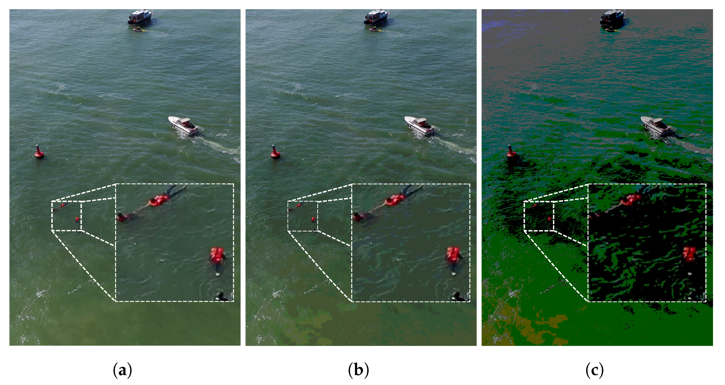
The quantization, also called bit depth or color depth, defines the number of different values per pixel and color (see Figure 1). Quantization is used to describe a continuous signal with discrete values [19]. Too few quantization steps lead to a significant error, resulting in a loss of information. Therefore, it is necessary to balance the required storage space and the information it contains.
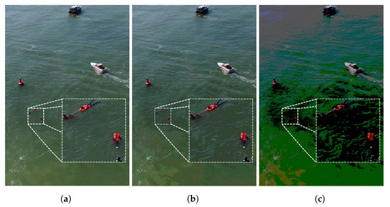
Figure 1.
Example images for Quantization.(a) 8 Bit; (b) 4 Bit; (c) 2 Bit.
All used data sets provide images with an 8 bit quantization. We want to evaluate whether we can reduce the bit depth further without losing performance. A smaller bit depth results in a smaller data size. Hence, 8 bit is the maximally available quantization of the data sets. We provide experiments for 8 bit, 4 bit, and 2 bit quantization. These decrease the size of the images for a bitmap format by the factors 2 (for 4 bit) and 4 (for 2 bit).
2.2.2. Compression
Compression is used to reduce the required space of a recording. There are two types of compressions: lossless and lossy compressions. The image format PNG belongs to lossless compression techniques. The compression time for PNG is very high. Therefore, it is not usable for online compression. JPEG is faster, but also a lossy compression. The compression removes information. Nevertheless, JPEG is a common choice. It provides a sufficient trade-off between loss of information, file size, and speed.
The compression quality of JPEG is defined as a value between 1 and 100 (default: 90). Higher values cause less compression.
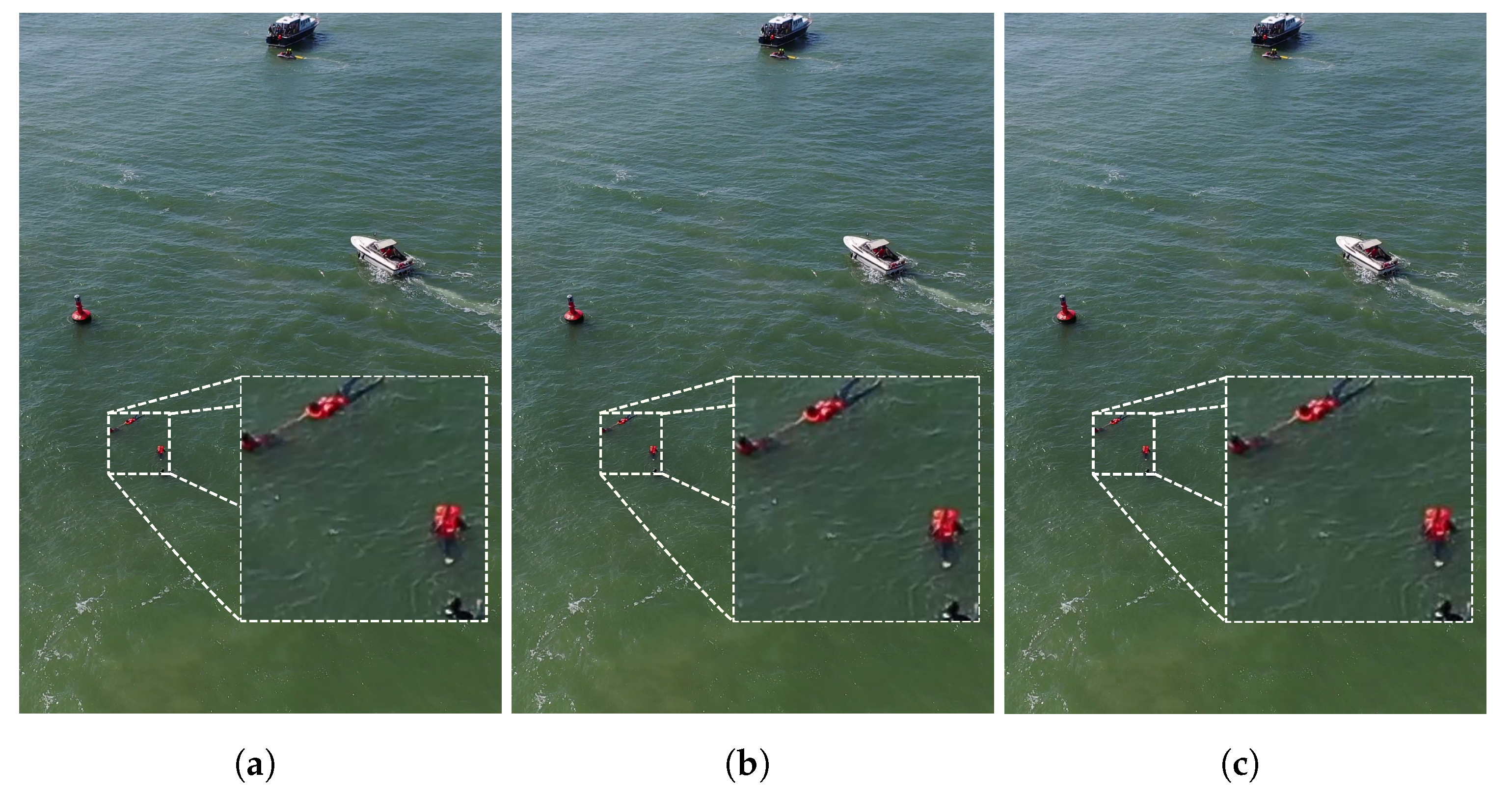
We check the relation between compression and detector performance. A lower compression quality would result in smaller file sizes. This directly leads to a higher throughput of the system. For the inferences of models, the decompressed data is used. A lower compression quality would, therefore, mainly affect the throughput from the camera to the processing unit memory. Since this is also a limiting factor for high-resolution or high-speed cameras, it is worth checking. In our experiments, we evaluate the influence of no compression and compression quality for JPEG of 90 and 70 (see Figure 2). The difference is difficult to see with the human eye, so we have included more examples in the Appendix D.3.
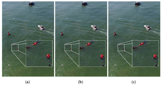
Figure 2.
Example images for Compression. (a) No comp.; (b) 90 comp. quality; (c) 70 comp. quality.
2.2.3. Color Model
The color model defines the representation of the colors. The most common is RGB [20]. It is an additive color model based on three colors red, green, and blue. For object detection and object classification, this representation is mostly used [14,16]. Besides RGB, non-linear transformations of RGB are also worth considering. HLS and HSV are based on a combination of hue and saturation. Both differ in the brightness’s definition value. YCbCr considers human perception and encodes information more suitably for humans.
In some applications, HSV outperforms RGB. Cucchiara et al. [21] and Shuhua et al. [22] could confirm this performance improvement. Kim et al. demonstrated RGB outperforms the other color models (HSV, YCbCr, and CIE Lab) in traffic signal detection. Which color model is best depends strongly on the application and the model.
The color model is also a design decision, so we evaluate the performance of RGB, HSV, HLS, and YCbCr color models for object detection in remote sensing. We also review the performance of gray-scale images. To achieve comparable results, the backbones are not pre-trained for these experiments.
2.2.4. Resolution
Higher resolutions reveal more details but also result in larger recordings. Especially for the small objects of remote sensing, the details are crucial [23]. Therefore, choosing an optimal resolution is important [24].
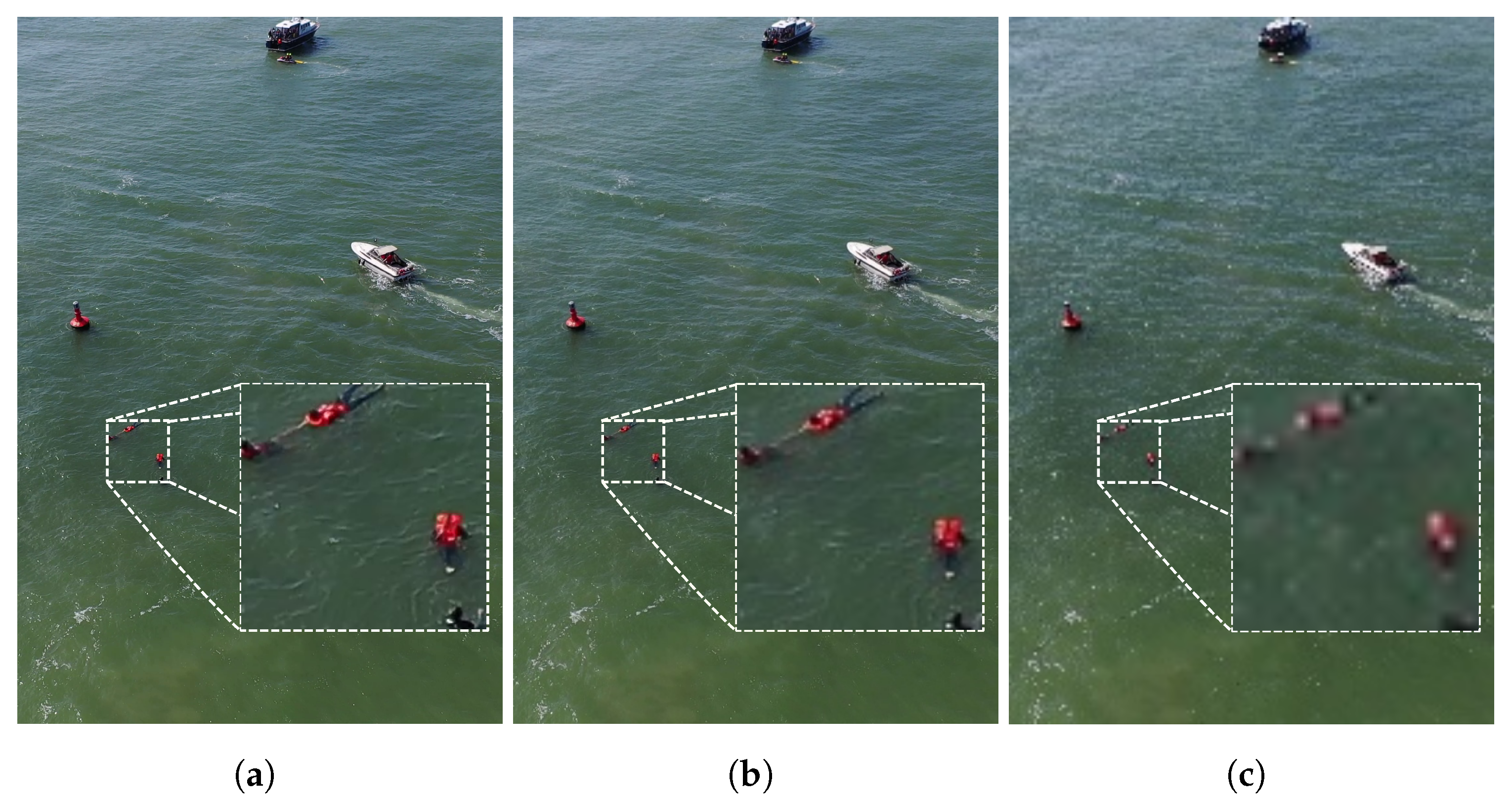
Besides the maximally available resolution defined by the used camera, the GPU memory often limits the training size. The reason lies in the gradient calculation within the backpropagation step. Some techniques reduce this problem [18,25]. To allow a fair comparison, we limit the maximum training size to 1024 pixels for the length of the larger side. This training size is processable with all models used. The experiments should show the performance reduction for smaller image sizes. So we trained on the training sizes of 256 pixels, 512 pixels, 756 pixels, and 1024 pixels (see examples in Figure 3). Further, we evaluated each training size with three test sizes, defined by the training size × the factors 0.5, 1, and 2.
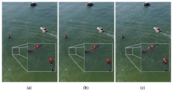
Figure 3.
Example images for image resolutions with max side length. (a) Full resolution; (b) Max 768 pixels; (c) Max 256 pixels.
2.2.5. Multispectral Recordings
In recent years, the usage of multispectral cameras on drones has gotten more popular [26,27,28]. These have additional channels, which increase the recording size, but can also provide important information. The additional channels normally lie outside the visible light (e.g., near-infrared or thermal). In pedestrian and traffic monitoring, multispectral imaging can increase the detector performance, as shown by Takumi et al. [29], Maarten et al. [30], and Dayan et al. [31]. And for precision agriculture, they are one of the key components [26,27,28]. We want to create awareness that multispectral recordings can be helpful in some situations. But we also want to check how easy integration into existing object detection pipelines is. So, the focus is not on evaluating multimodal models [32]. Our experiments are limited to the early fusion approach [33] as we see multispectral recordings as a special case of color images.
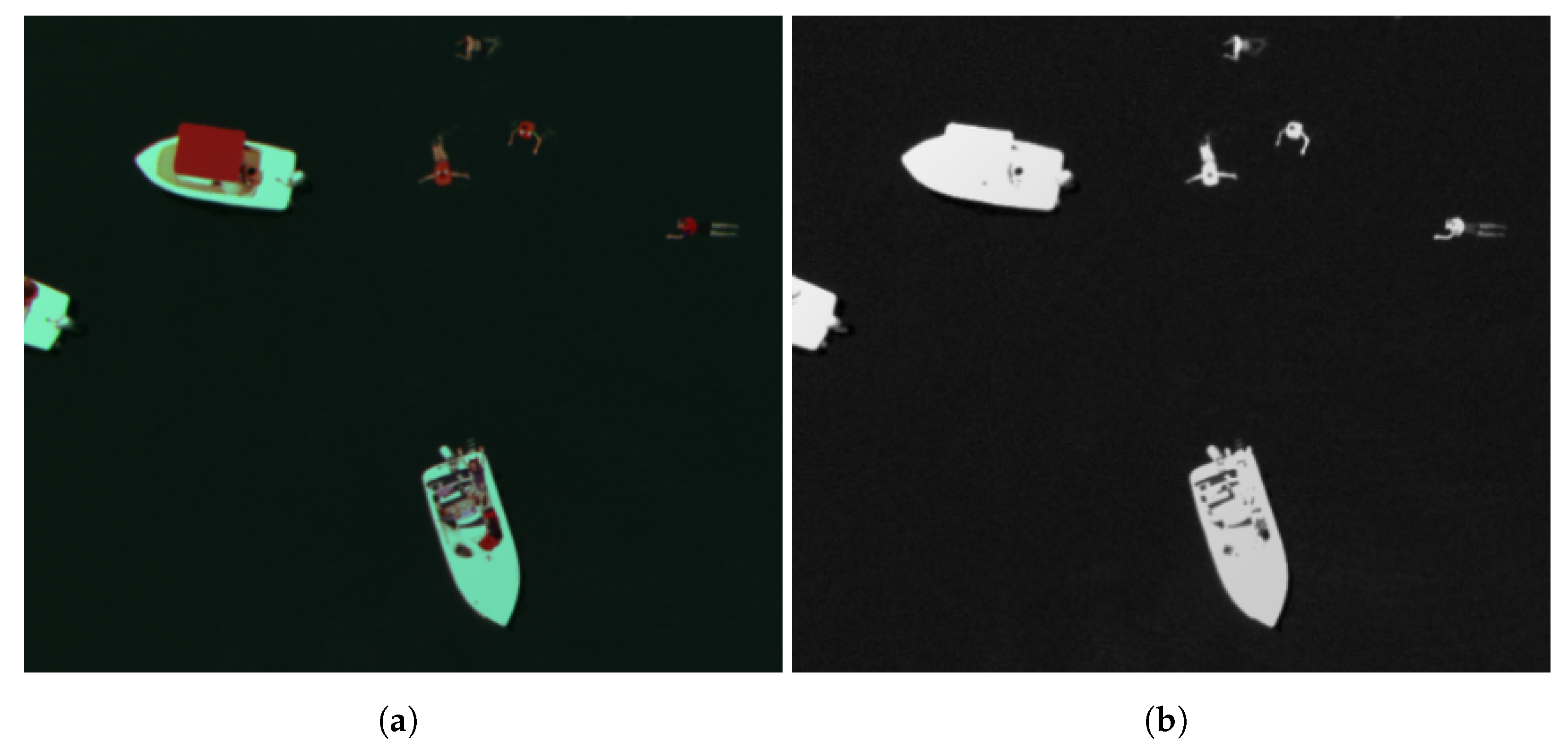
We used multispectral images from the SeaDronesSee [2] data set for our experiments. These were acquired with a MicaSense RedEdge MX and thus provided wavelengths of 475 nm (blue), 560 nm (green), 668 nm (red), 717 nm (red edge), and 842 nm (near infrared). We evaluate how the additional wavelengths affect the performance of the object detectors in detecting swimmers. In theory, the near-infrared channel provides a foreground mask for objects in water (see example in Figure 4). These experiments should provide a general trend, even if the exact results apply only to the maritime environment. It is worth considering if additional channels could carry helpful information.
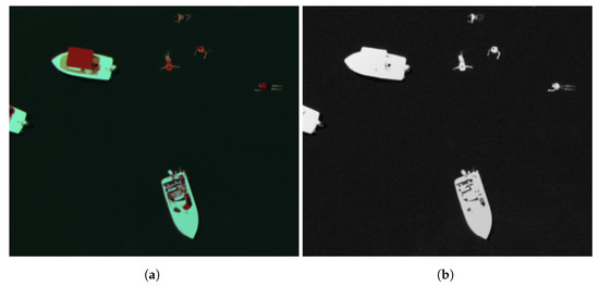
Figure 4.
Example images for multispectral recordings in maritime environment. In the NIR recordings, the swimmers are fully visible. (a) RGB; (b) Near-infrared.
2.2.6. Calibration Parameters
We look on two calibration parameters, image distortion and gamma correction.
Image Distortion
During the image formation process, most lenses introduce a distortion in the digital image that does not exist in the scene [34]. Wide-angle lenses or fish-eye lenses suffer from the so-called barrel-distortion, where image magnification decreases with distance from the optical axis. Telephoto lenses suffer from the so-called pincushion-distortion, where the image magnification increases with distance to the optical axis.
One of the first steps in image processing pipelines is often to correct the lens distortion using a reference pattern.
As we are working on data sets that are distortion rectified, we artificially introduce distortion via the Brown–Conrady model [35]. To evaluate the impact of an incorrect calibration, we introduce a small barrel-distortion with and pincushion-distortion with . A visualization of these distortions can be found in Appendix D.2.
Gamma Correction
Most cameras use an auto-exposure setting, which adjusts the camera exposure to the ambient lighting. But manual exposure is still common and can result in overexposed (too bright) or underexposed (too dark) images. Gamma correction can ease this problem, but it can also be used to simulate a camera in a wrong exposure setting.
Gamma Correction is a non-linear operation to encode and decode luminance to optimize the usage of bits when storing an image by taking advantage of the non-linear manner in which humans perceive light and color [36]. Gamma Correction can also simulate a shorter or longer exposure process after the image formation process. In the simplest case, the correction is defined by a power function, which produces darker shadows for a gamma value smaller than one and brighter highlights with a gamma value larger than one. If images are not gamma-corrected, they allocate too many bits for areas humans cannot differentiate. Humans perceive changes in brightness logarithmically [37]. Contrarily, neural networks, however, work with floating points, making them sensitive to minimal changes in quantization, as can be observed in many works that examine weight quantization [38,39,40]. We, therefore, assume that Gamma Correction may have a negligible impact on neural network detection performance.
Many works have employed Gamma Correction to improve detection performance directly or help training with Gamma Correction as an augmentation technique [41,42].
We use three different gamma configurations (0.5, 1.0, and 2.5) to investigate the effects of gamma on the object detector performance. These experiments are designed to show whether gamma is a crucial parameter. The performance of a dynamic gamma adjustment [43] was also be tested.
3. Results
Each parameter is considered in its subsection. The experiments of the different backbones per network were grouped. Only the largest backbones of CenterNet and Faster R-CNN are listed separately. We use the mean Average Precision (mAP) as a metric with an intersection over union (IoU) threshold of 0.5 [44]. The mean Average Precision metric averages the precision values of the predictions over the recall values and all classes. The IoU threshold defines the minimum overlap between a prediction and a ground-truth bounding box to be counted as a positive sample. It is the most common metric to measure the performance of object detectors.
For the Dota data set, the performance of the models differs from the performance in the other data sets. The objects in the Dota data set are tiny. As a result, it challenges the object detectors differently.
3.1. Quantization
A quantization reduction leads to a loss of information in the recording. This assumption is confirmed by the empirical results in Figure 5. This phenomenon is consistent for all data sets and all models. However, deterioration varies.

Figure 5.
Quantization: the impact of the quantization on the performance of the object detectors for all data sets. The y-axis shows the mean Average Precision (mAP).
The marginal difference (∼3%) in performance between 4 bit and 8 bit recordings is worth mentioning. Hence, it is possible to have half the data and achieve nearly the same result. The loss in performance for a 2 bit quantization is much higher (∼41%).
3.2. Compression
Figure 6 shows the relation between compression quality and object detector performance. Lower compression quality, i.e., higher compression, leads to worse performance. With some exceptions, this is true for all models. Overall, the performance degeneration of the tested compression qualities is slight. For a compression quality of 90, the performance is decreased by ∼2.7%. A compression quality of 70 leads to an mAP loss of ∼5.3%. Compared to the performance loss, the size reduction is significant.

Figure 6.
Compression: the impact of the JPEG compression on the performance of the object detectors for all data sets. The y-axis shows the mean Average Precision (mAP). A higher compression quality means less compression.
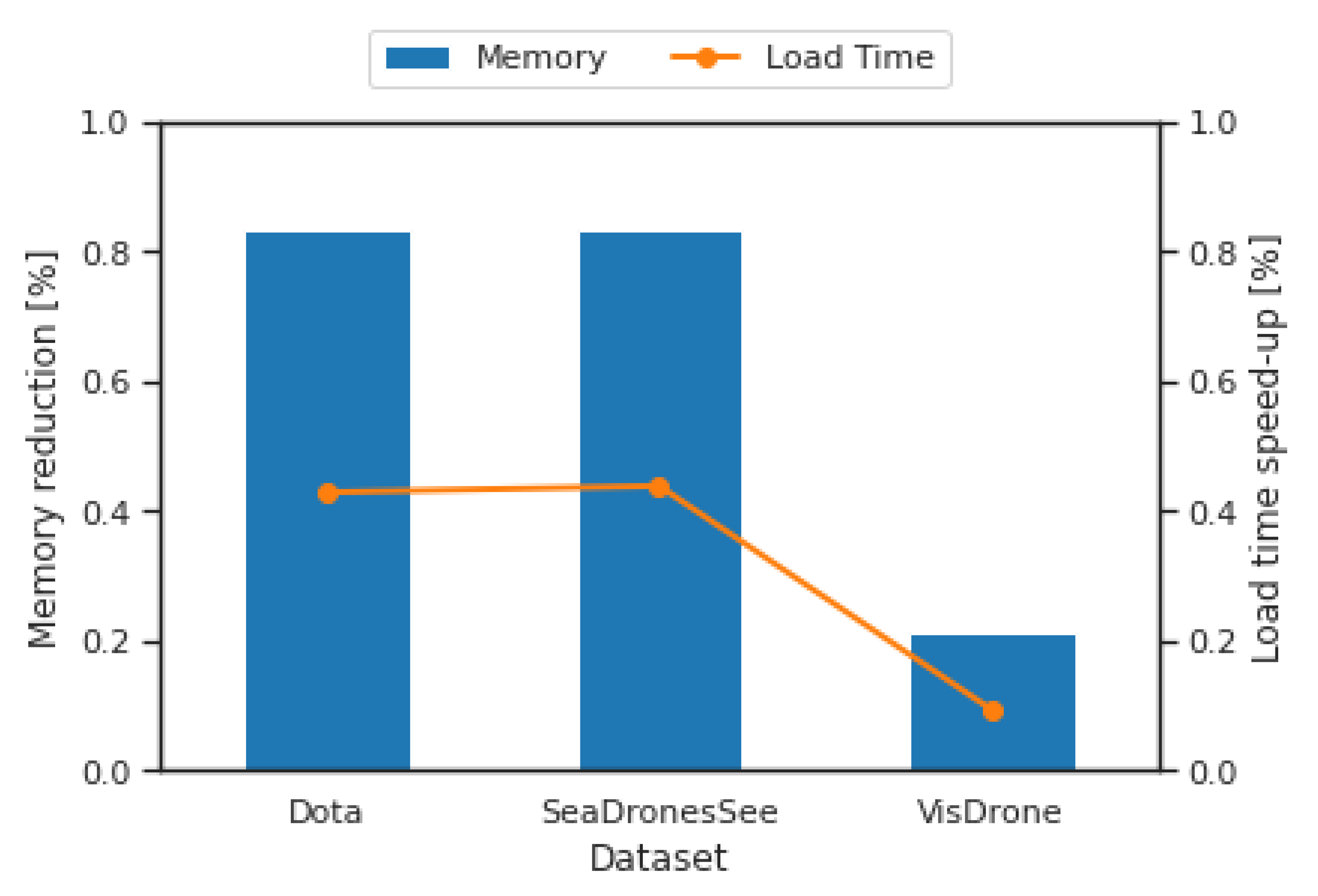
We observe that a compression quality of 90 reduces the required space by ∼22% for a random subset of the VisDrone validation set. A compression quality of 70 can almost halve the required space. However, memory reduction depends highly on the image content. For SeaDronesSee and Dota, the memory reduction is much higher. For compression quality of 70 and 90, it is about ∼93% and ∼83%, respectively. By reducing the required image space, it is possible to increase the pipeline throughput. In return, compression and decompression are necessary. In the final experiments, the utility of this approach becomes apparent.
3.3. Color Model
We can conclude two essential outcomes of the experiment for color models. First, we must distinguish between two situations visible in Figure 7. In the first situation, the object detectors cannot take advantage of the color information. Therefore, we assume the color is, in this case, not beneficial. This applies to the VisDrone data set and the Dota data set. Both data sets provide objects and backgrounds with a high color variance. For example, a car in the VisDrone data set can have any color. Thus, the texture and shape are more relevant. That means the object detector can already achieve excellent results with the gray-scale recordings. The color information for the Dota data set could only be utilized by the largest models (Faster R-CNN/ResNext101_32x8d and CenterNet/Hourglass104). The other models couldn’t incorporate color and relied only on texture or shape.

Figure 7.
Color Model: the impact of the color models. The y-axis shows the mean Average Precision (mAP).
In the SeaDronesSee experiments, we observed that the color experiments outperform the gray-scale experiments. The explanation can be found in the application. It covers a maritime environment. As a result, the background is always a mixture of blue and green. So, the color information is reliable in distinguishing between background and foreground. For SeaDronesSee, all models use color, which is evident in the drop in performance for the gray-scale experiments.
If the color is essential, RGB produces the best results, followed by YCrCb. However, since most data augmentation pipelines have been optimized for RGB, we recommended using RGB as the first choice.
In conclusion, knowing whether color information is relevant in the application is crucial. Gray-scale images are usually sufficient, leading to a third of the image size, and may even allow more straightforward cameras.
3.4. Resolution
For these experiments, we only visualize the experiments of Faster R-CNN. The three selected plots (visible in Figure 8) represent the other models well because all follow a similar trend. The other plots can be found in the Appendix D.4.

Figure 8.
Image Size: Faster R-CNN trained with different training image sizes and validated on . The y-axis shows the mean Average Precision (mAP).
First, higher training resolutions consistently improve the performance of the models. Aside from that, the performance deterioration for a decreased validation image size is consistent over all experiments.
For the Dota data set, we can observe a performance drop for a higher test-size-scale factor. The trained models seem very sensitive to object sizes and cannot take advantage of higher resolutions. For the SeaDronesSee data set, performance improves with higher validation image sizes for most models. So it is possible to enhance the performance of a trained model by simply using higher inference resolutions. However, the improvement is marginal and should be supported by scaling data augmentation during training. The results for the SeaDronesSee data set also apply to the VisDrone data set. Only for the training image size of 1024 pixels does this rule not hold. The reason for this is the small number of high-resolution images in the VisDrone validation set.
In summary, training and validation sizes are crucial, and it is not a good idea to cut corners at this point. This applies to common objects, but is even more critical for the small objects of remote sensing.
3.5. Multispectral Recordings
These experiments are based on multispectral data of the SeaDronesSee data set. The usefulness of the additional channels depends strongly on the application. For the maritime environment, additional information is beneficial, especially in the near-infrared channel. This wavelength range is absorbed by water [45], resulting in a foreground mask (an example is shown in Figure 4).
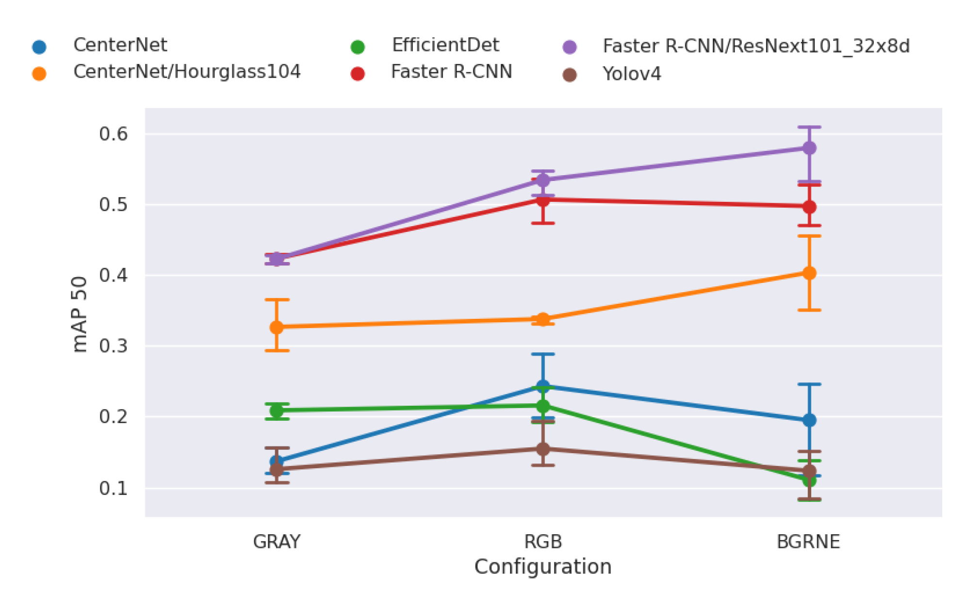
The results in Figure 9 fit to the findings for the color models (see Section 3.3). For the maritime environment, color information is important, as indicated by the gap for gray-scale recordings. The multispectral recordings (labeled as ‘BGRNE’) can only improve the performance of the larger models. For the smaller models, it even leads to a decrease in performance. To support the multispectral recordings as input, we had to increase the input channels of the first layer and lose the pretraining of this layer. The rest of the backbone is still pre-trained.
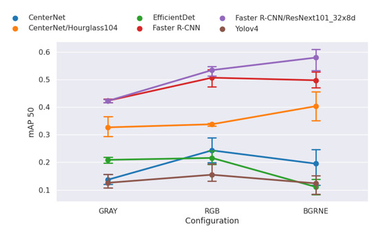
Figure 9.
Multispectral: the performance of the object detectors on multispectral data. (’BGRNE’—multispectral recordings, ’RGB’—color images, ’GRAY’—gray-scale).
In summary, additional channels can be helpful depending on the use case. It is essential to remember that larger backbones can better use the extra channels. Furthermore, it is a trade-off between a fully pre-trained backbone and additional information.
3.6. Camera Calibration
In our experiments, we observe that gamma correction and image distortion effects are equal across all data sets and models. Table 1 shows that applying (dynamic) gamma correction to the data sets seems to have a negligible/negative effect on detection accuracy. This implies that gamma correction indeed does not have a notable impact on detection accuracy.

Table 1.
Gamma Correction: impact on the performance.
Image distortion also seems to have a minimal effect on detection accuracy, as seen in Table 2. However, the models evaluated on images distorted using pincushion distortion achieved slightly higher accuracy. But although the mean performance over all data sets and models is higher for images with pincushion distortion, most of the models perform best when evaluated with no distortion, as can be seen in Appendix D.2 where we provide a detailed analysis.

Table 2.
Image Distortion: impact on the performance.
We can conclude that camera calibration is an existential part of many computer vision applications. However, the investigated correction methods affect only marginally the performance in remote sensing applications.
Finally, we showed that the optimized parameters can be utilized to deploy a UAV-based prototype (displayed in Figure 10) with nearly real-time and high-resolution processing.

Figure 10.
Prototype system using an optimized detection pipeline. (a) Original input and optimized input; (b) Detection pipeline onboard a DJI Matrice 100.
4. Discussion
In the previous experiments, we showed that the inspected parameters have an unequal impact on the performance of a model. Some have a minor effect on the performance but significantly impact the required space (quantization, compression). Others have a negligible influence on the performance (color model, calibration parameters). Furthermore, others are fundamental for the remote sensing application (resolution). Further, in Section 3.5, we showed that more complex camera systems, e.g., multispectral cameras, can boost performance. However, only if the additional channels carry helpful information, as discussed using the example of detecting swimmers in a maritime environment in Section 2.2.5. As a result, we want to emphasize keeping the whole object detection pipeline in mind when building an object detection system.
As the parameters have an unequal impact on the performance, we can reduce the memory consumption of the parameters, which have a minor effect on the performance. The freed space can be used to increase the throughput of the system or can be utilized to boost the crucial parameters by assigning more memory space to these.
We determine the optimal parameter configuration for the remote sensing application based on previous investigations and assumptions. These parameters are proposed as a recommendation for future work. The objective was to find a suitable compromise between the detection performance and the required space for a recording, which limits the pipeline’s throughput and defines the frames per second of the system. The combination of the optimal parameters utilizes the pipeline more efficiently. For a maximal throughput with a negligible loss of performance, we recommend the following:
- A quantization reduction from 8 bit to 4 bit is sufficient, as the models do not utilize the entire color spectrum. This was shown in Section 3.1.
- A JPEG compression with a compression quality of 90 reduces the performance slightly but reduces the memory footprint significantly. This was concluded of the results in Section 3.2.
- For the urban surveillance use-case, color is not essential. Thus, for the VisDrone data set, we recommend gray-scale images. For the other data sets, the color is important. This recommendation is based the results in Section 3.3.
The mentioned recommendations lead to a reduction in memory consumption. This could be used to increase the frames per second of the system. In Table 3, this thesis is proven. The first setup (marked *), which uses the reduced quantization, the JPEG compression, and the optional color reduction, significantly increases the throughput (including the inference and the pre-and post-processing) of the smaller models. In contrast to the baselines, we speed up the detection pipeline (≈+15%) with a small loss in performance (≈). For the larger models, inference accounts for most of the throughput, so there is no significant speed-up. In Appendix D.5, we show the loading speed improvement when working with optimized images for the three data sets.

Table 3.
Application of the optimized parameter configuration in a desktop and an embedded environment: The mean Average Precision (mAP) are presented for the data sets and the models. For each model, at least two configurations are given (baseline and optimized pipeline). Frames per second (FPS) indicate the inference speed of each model. In the last column, the number of trainable parameters is given. The percentages in the parentheses indicate the change regarding the baseline.
If the best performance is the target of the project. We recommend utilizing the freed space with the additional recommendation:
- 4
- Utilize the highest possible resolution because this is a crucial parameter for small objects of remote sensing applications. This was concluded of the experiments in Section 3.4
Combining the first three adjustments and increasing the resolution (marked **) in Table 3, the detector’s performance can be improved (≈+25%) while maintaining the base throughput. In these experiments, the usage of CroW, described in Section 2.1.2, allowed training with higher resolution.
Further, we can conclude the following statements based on the experiments. These do not affect the trade-off between performance and throughput but are still important for future projects.
- 5
- As has been shown in Section 3.6, a minor error in the camera calibration (distortion or gamma) is not critical.
- 6
- In specific applications, multispectral cameras can be helpful. For example, we have shown in Section 3.5, that multispectral recordings boost the performance in maritime environments.
5. Conclusions
This paper extensively studies parameters that should be considered when designing an entire object detection pipeline in a UAV use case. Our experiments show that not all parameters have an equal impact on detection performance, and a trade-off can be made between detection accuracy and data throughput.
By using the above recommendations, it is possible to maximize the efficiency of the object detection pipeline in a remote sensing application.
In future work, we want to explore recording data with varying camera parameters. This would allow evaluating even more parameters like camera focus or exposure. Also, a deeper analysis of the usability of multispectral imaging could provide valuable insights.
Author Contributions
Conceptualization, L.A.V.; methodology, L.A.V. and S.K.; software, L.A.V. and S.K.; validation, L.A.V. and S.K.; formal analysis, L.A.V. and S.K.; investigation, L.A.V. and S.K.; resources, L.A.V.; data curation, L.A.V.; writing—original draft preparation, L.A.V. and S.K.; writing—review and editing, L.A.V. and S.K.; visualization, L.A.V. and S.K.; supervision, L.A.V. and A.Z.; project administration, L.A.V.; funding acquisition, A.Z. All authors have read and agreed to the published version of the manuscript.
Funding
The German Ministry for Economic Affairs and Energy has supported this work, Project Avalon, FKZ: 03SX481B. The computing cluster of the Training Center Machine Learning, Tübingen has been used for the evaluation, FKZ: 01IS17054.
Data Availability Statement
The full list of experiement results can be on: https://github.com/cogsys-tuebingen/cp_eval (accessed on 10 September 2022).
Conflicts of Interest
The authors declare no conflict of interest.
Abbreviations
The following abbreviations are used in this manuscript:
| ADAS | Advanced Driver Assistance System |
| FPS | Frames Per Second |
| IoU | Intersection over Union |
| mAP | mean Average Precision |
| MAV | Mirco Aerial Vehicle |
| UAV | Unmanned Aerial Vehicle |
Appendix A. Data Sets
Appendix A.1. Dota-2
Ding et al. provide high-resolution satellite images with annotations [3]. We used the recommended preprocessing technique to create 1024 × 1024 tiles of the high-resolution recordings. This results in 8615 training images with 449,407 annotations. All the recordings are provided in the lossless PNG format. Some images contain JPEG compression artifacts, so we assume that not the entire data set creation pipeline was lossless. The reported accuracy is evaluated on the validation set (with 2619 images) as the test set is not publicly available.
Appendix A.2. SeaDronesSee-DET
SeaDronesSee focus on search and rescue in maritime environments [2]. The training set includes 2975 images with 21,272 annotations. We reduced the maximum side length of the images to 1024 pixels for this data set.
The reported accuracy is evaluated on the test set (with 1796 images). This data set uses the PNG format [46], which utilizes a lossless compression.
Appendix A.3. VisDrone-DET
Zhu et al. proposed one of the most prominent UAV recordings data set [1]. The focus of this data set is traffic surveillance in urban areas. We use the detection task (VisDrone-DET). The training set contains 6471 images with 343,205 annotations. Unless otherwise mentioned, we reduced the maximum side length by down-scaling to 1024 pixels.
We used the validation set for evaluation, as the test set is not publicly available. The validation set contains 548 images. All images of this data set are provided in JPEG format [47] with a compression quality of 95.
Appendix B. Models
Appendix B.1. CenterNet
Duan et al. proposed CenterNet [17], an anchor-free object detector. The network uses a heat-map to predict the center-points of the objects. Based on these center-points, the bounding boxes are regressed. Hourglass-104 [48] is a representative for extensive backbones, while the ResNet-backbones [49] cover a variety of different backbone sizes. The ResNet backbones were trained with Adam and a learning rate of . Further, we also used the plateau learning scheduler. For the Hourglass104-backbone, we used the learning schedule proposed by Pailla et al. [50].
Appendix B.2. EfficientDet
EfficientDet is optimized for efficiency and can perform well with small backbones [16]. Even though there is an EfficentNetV2 announced, which should be more efficient as backbone [51], there is currently, to the best of our knowledge, no object detector using this backbone. For our experiments, we used EfficientDet with two backbones. The -backbone is the smallest and fastest of this family. And the -backbone represents a good compromise between size and performance. We used three anchor scales (0.6, 0.9, 1.2), which are optimized to detect the small objects of the data sets. For the optimization, we used an Adam optimizer [52] with a learning rate of . Further, we used a learning rate scheduler, which reduces the learning rate on plateaus with patience of 3 epochs.
Appendix B.3. Faster R-CNN
Faster R-CNN is the most famous two-stage object detector [14]. And many of its improvements achieve today still state-of-the-art results [1]. We use three backbones for Faster R-CNN. A ResNet50 and a ResNet101 of the ResNet-family [49]. Also, a ResNeXt101 backbone [53] For Faster R-CNN, we use the Adam optimizer [52] with a learning rate of and a plateau scheduler.
Appendix B.4. Yolov4
Bochkovskiy et al. published YoloV4 [15], which is the latest member of the Yolo-family providing a scientific publication. Besides a comprehensive architecture and parameter search, they did an in-depth analysis of augmentation techniques, called ‘bag of freebies’, and introduced the Mosaic data augmentation technique. YoloV4 is a prominent representative of the object detectors because of impressive results on MS COCO. By default, YoloV4 scales all input images down to an image size of 608 × 608 pixels. For our experiments, we removed this preprocessing to improve the prediction of smaller objects.
Appendix C. Hardware Setup
Appendix C.1. Desktop Environment
The models were trained on computing nodes equipped with four GeForce GTX 1080 Ti graphic cards. The system was based on the Nvidia driver (version 460.67), CUDA (version 11.2) and PyTorch (version 1.9.0). To evaluate the inference speed in a desktop environment, we used a single RTX 2080 Ti with the same driver configuration.
Appendix C.2. Embedded Environment
The Nvidia Xavier AGX provides 512 Volta GPU cores, which are the way to go for the excessive forward passes of the neural networks. Therefore, it is a flexible way to bring deep learning approaches into robotic systems. We used the Nvidia Jetpack SDK in the version 4.6, which is shipped with TensorRT 8.0.1. TensorRT can speed up the inference of trained models. It optimizes these for the specific system, making it a helpful tool for embedded environments. For all embedded experiments, the Xavier board was set to the power mode ’MAXN’, which consumes around 30 W and utilizes all eight CPUs. Further, it makes use of the maximum GPU clock rate of around 1377 MHz.
Appendix D. Additional Examples
In this appendix, additional example images and further information on the considered factors of influence are provided.
Appendix D.1. Quantization
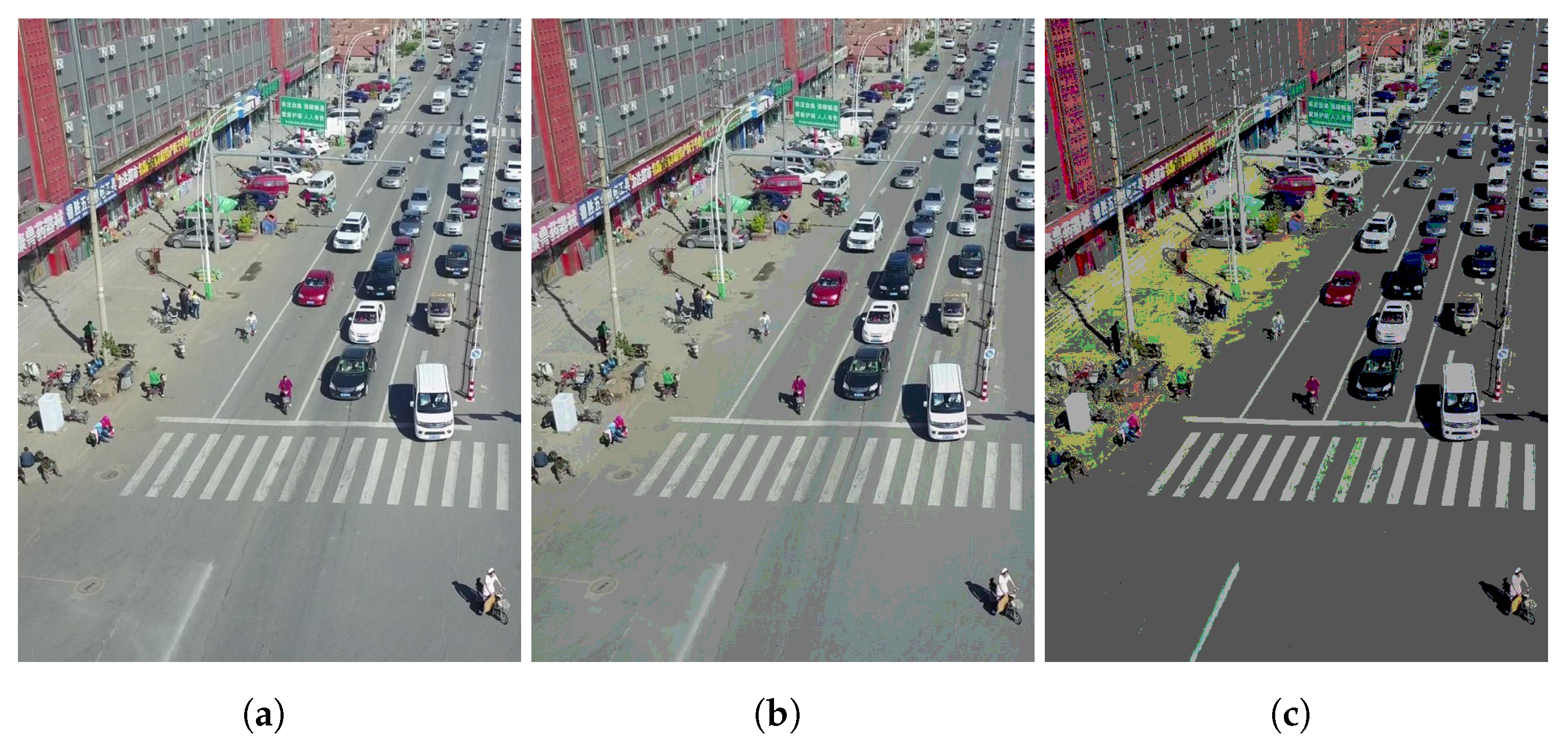
Figure A1 shows different quantization configurations. The differences are visible by the human eye. Already, the 4 bit quantization seems not fully realistic for human perception.
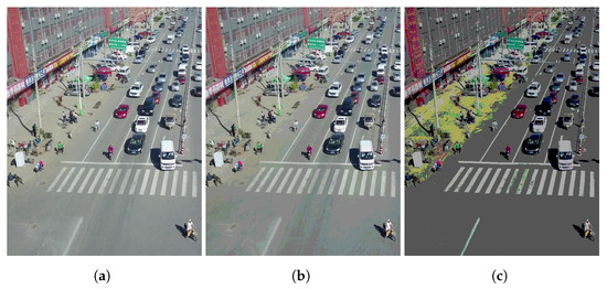
Figure A1.
Example images for Quantization. (a) 8 bit; (b) 4 bit; (c) 2 bit.
Figure A1.
Example images for Quantization. (a) 8 bit; (b) 4 bit; (c) 2 bit.
Appendix D.2. Calibration Parameters
The used distortion is easily recognizable on the checkerboard pattern (see Figure A2).

Figure A2.
Reference distortion used in the paper, visualized by a checkerboard pattern. From left to right: Pincushion distortion, no distortion, barrel distortion.
Figure A2.
Reference distortion used in the paper, visualized by a checkerboard pattern. From left to right: Pincushion distortion, no distortion, barrel distortion.

Figure A3 shows the rectified image and two not optimal setups. In (a), the image is overexposed and the barrel distortion of the lens was not fully corrected. In setup (c), the image is underexposed, and the recording is affected by a pincushion distortion. In a real world image, the distortions are hard to see. They are only visible for straight lines (like for the checkerboard). In contrast, the incorrect exposure, which correlates with the gamma value, is obvious. In Figure A4 the breakdown of the image distortion impact on the different data sets and models is visualized. Figure A5 shows the same for the impact of gamma. The difference in performance for varying distortion and gamma levels is minor, as already described in the main paper. Not all models are affected equally by changing distortion or gamma, but most often no distortion and unaltered gamma performs best.
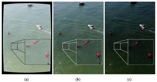
Figure A3.
Example images for Camera Calibration. (b) Rectified. (a) and (c) mimic invalid exposure time and lense distortion.
Figure A3.
Example images for Camera Calibration. (b) Rectified. (a) and (c) mimic invalid exposure time and lense distortion.
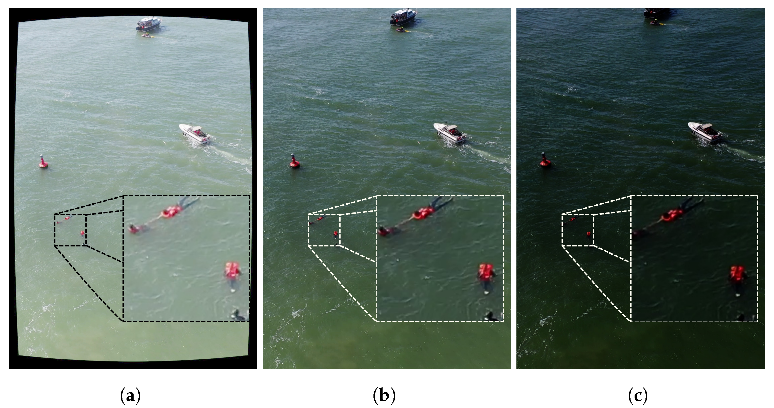

Figure A4.
Image Distortion: the impact of the image distortion on the performance of the object detectors for all data sets. The y-axis shows the mean Average Precision (mAP).
Figure A4.
Image Distortion: the impact of the image distortion on the performance of the object detectors for all data sets. The y-axis shows the mean Average Precision (mAP).


Figure A5.
Image Gamma: the impact of the gamma on the performance of the object detectors for all data sets. The y-axis shows the mean Average Precision (mAP).
Figure A5.
Image Gamma: the impact of the gamma on the performance of the object detectors for all data sets. The y-axis shows the mean Average Precision (mAP).

Appendix D.3. Compression
In Figure A6 the influence of different JPEG compression qualities is visible. For the compression qualities, which were used for the main evaluation (90, 70), it is hard to see the compression artifacts with the human eye. Therefore, the additional compression qualities (50, 20, 10) are presented. Especially, for the lowest used compression quality (10) the typical JPEG compression artifacts are noticeable (unsharp corners, squares with incorrect color).
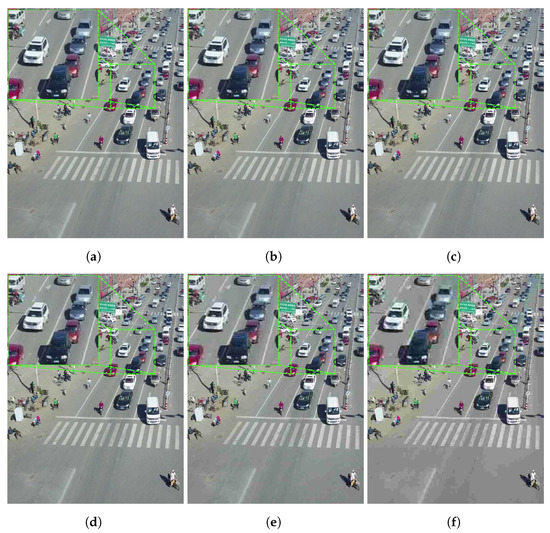
Figure A6.
Example images for JPEG compression. (a) No comp.; (b) 90 comp. quality; (c) 70 comp. quality; (d) 50 comp. quality; (e) 20 comp. quality; (f) 10 comp. quality.
Figure A6.
Example images for JPEG compression. (a) No comp.; (b) 90 comp. quality; (c) 70 comp. quality; (d) 50 comp. quality; (e) 20 comp. quality; (f) 10 comp. quality.
Appendix D.4. Resolution
In Figure A7 an image with different resolutions is shown. For smaller resolution, the detection of smaller objects is especially hard. These can vanish completely. Large and medium objects normally lose only features, which makes the detection harder but not impossible. Therefore, the impact on smaller objects seems higher.
Figure A8, Figure A9 and Figure A10, the behavior of the different models for the tested image resolutions is visible. All models follow the trend of Faster RCNN, which was described in the main analysis. EfficientDet seems more sensitive to resolution changes than the other models.

Figure A7.
Example images for image resolutions with max side length. (a) Full res.; (b) Max 768 pixels; (c) Max 512 pixels; (d) Max 256 pixels; (e) Max 128 pixels.
Figure A7.
Example images for image resolutions with max side length. (a) Full res.; (b) Max 768 pixels; (c) Max 512 pixels; (d) Max 256 pixels; (e) Max 128 pixels.
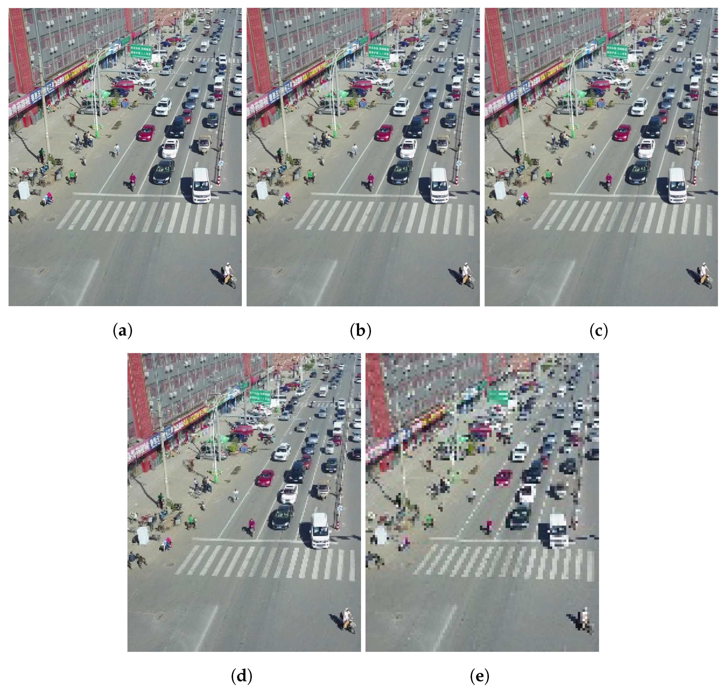

Figure A8.
Image Size: CenterNet trained with different training image sizes and validated on . The y-axis shows the mean Average Precision (mAP).
Figure A8.
Image Size: CenterNet trained with different training image sizes and validated on . The y-axis shows the mean Average Precision (mAP).


Figure A9.
Image Size: EfficientDet trained with different training image sizes and validated on . The y-axis shows the mean Average Precision (mAP).
Figure A9.
Image Size: EfficientDet trained with different training image sizes and validated on . The y-axis shows the mean Average Precision (mAP).


Figure A10.
Image Size: YoloV4 trained with different training image sizes and validated on . The y-axis shows the mean Average Precision (mAP).
Figure A10.
Image Size: YoloV4 trained with different training image sizes and validated on . The y-axis shows the mean Average Precision (mAP).

Appendix D.5. Speed-Up Comparison
Figure A11 shows the direct correlation between memory reduction and speed-up for the three data sets. The difference in memory reduction for the data sets is significant. For SeaDronesSee and Dota the reduction is much higher.

Figure A11.
Space reduction and loading time speed-up for the different data sets compared.
Figure A11.
Space reduction and loading time speed-up for the different data sets compared.
References
- Zhu, P.; Wen, L.; Du, D.; Bian, X.; Hu, Q.; Ling, H. Vision Meets Drones: Past, Present and Future. CoRR 2020, abs/2001.06303. [Google Scholar]
- Varga, L.A.; Kiefer, B.; Messmer, M.; Zell, A. SeaDronesSee: A maritime benchmark for detecting humans in open water In Proceedings of the IEEE/CVF Winter Conference on Applications of Computer Vision (WACV), Waikoloa, HI, USA, 3–8 January 2022. pp. 2260–2270.
- Ding, J.; Xue, N.; Xia, G.; Bai, X.; Yang, W.; Yang, M.Y.; Belongie, S.J.; Luo, J.; Datcu, M.; Pelillo, M.; et al. Object Detection in Aerial Images: A Large-Scale Benchmark and Challenges. CoRR 2021, abs/2102.12219. [Google Scholar] [CrossRef]
- Yahyanejad, S.; Misiorny, J.; Rinner, B. Lens distortion correction for thermal cameras to improve aerial imaging with small-scale UAVs. In Proceedings of the 2011 IEEE International Symposium on Robotic and Sensors Environments (ROSE), Montreal, QC, Canada, 17–18 September 2011; pp. 231–236. [Google Scholar] [CrossRef]
- Blasinski, H.; Farrell, J.E.; Lian, T.; Liu, Z.; Wandell, B.A. Optimizing Image Acquisition Systems for Autonomous Driving. Electron. Imaging 2018, 2018, 161-1–161-7. [Google Scholar] [CrossRef]
- Carlson, A.; Skinner, K.A.; Vasudevan, R.; Johnson-Roberson, M. Modeling Camera Effects to Improve Visual Learning from Synthetic Data. In Proceedings of the Computer Vision—ECCV 2018 Workshops, Munich, Germany, 8–14 September 2018; Springer: Cham, Switzerland, 2019; Volume 11129, pp. 505–520. [Google Scholar] [CrossRef]
- Liu, Z.; Lian, T.; Farrell, J.E.; Wandell, B.A. Soft Prototyping Camera Designs for Car Detection Based on a Convolutional Neural Network. In Proceedings of the IEEE/CVF International Conference on Computer Vision (ICCV), Seoul, Korea, 27 October–2 November 2019; pp. 2383–2392. [Google Scholar] [CrossRef]
- Liu, Z.; Lian, T.; Farrell, J.E.; Wandell, B.A. Neural Network Generalization: The Impact of Camera Parameters. IEEE Access 2020, 8, 10443–10454. [Google Scholar] [CrossRef]
- Saad, K.; Schneider, S. Camera Vignetting Model and its Effects on Deep Neural Networks for Object Detection. In Proceedings of the 2019 IEEE International Conference on Connected Vehicles and Expo (ICCVE), Graz, Austria, 4–8 November 2019; pp. 1–5. [Google Scholar] [CrossRef]
- Secci, F.; Ceccarelli, A. On failures of RGB cameras and their effects in autonomous driving applications. In Proceedings of the 2020 IEEE 31st International Symposium on Software Reliability Engineering (ISSRE), Coimbra, Portugal, 12–15 October 2020. [Google Scholar] [CrossRef]
- Buckler, M.; Jayasuriya, S.; Sampson, A. Reconfiguring the Imaging Pipeline for Computer Vision. In Proceedings of the IEEE International Conference on Computer Vision (ICCV), Venice, Italy, 22–29 October 2017; pp. 975–984. [Google Scholar] [CrossRef]
- Li, R.; Wang, Y.; Liang, F.; Qin, H.; Yan, J.; Fan, R. Fully Quantized Network for Object Detection. In Proceedings of the IEEE/CVF Conference on Computer Vision and Pattern Recognition (CVPR), Long Beach, CA, USA, 15–19 June 2019; pp. 2810–2819. [Google Scholar] [CrossRef]
- Cai, Y.; Yao, Z.; Dong, Z.; Gholami, A.; Mahoney, M.W.; Keutzer, K. ZeroQ: A Novel Zero Shot Quantization Framework. In Proceedings of the IEEE/CVF Conference on Computer Vision and Pattern Recognition (CVPR), Seattle, WA, USA, 13–19 June 2020; pp. 13166–13175. [Google Scholar] [CrossRef]
- Ren, S.; He, K.; Girshick, R.B.; Sun, J. Faster R-CNN: Towards Real-Time Object Detection with Region Proposal Networks. IEEE Trans. Pattern Anal. Mach. Intell. 2017, 39, 1137–1149. [Google Scholar] [CrossRef]
- Bochkovskiy, A.; Wang, C.; Liao, H.M. YOLOv4: Optimal Speed and Accuracy of Object Detection. CoRR 2020, abs/2004.10934. [Google Scholar]
- Tan, M.; Pang, R.; Le, Q.V. EfficientDet: Scalable and Efficient Object Detection. In Proceedings of the IEEE/CVF Conference on Computer Vision and Pattern Recognition (CVPR), Seattle, WA, USA, 13–19 June 2020; pp. 10778–10787. [Google Scholar] [CrossRef]
- Duan, K.; Bai, S.; Xie, L.; Qi, H.; Huang, Q.; Tian, Q. CenterNet: Keypoint Triplets for Object Detection. In Proceedings of the IEEE/CVF International Conference on Computer Vision (ICCV), Seoul, Korea, 27 October–2 November 2019; pp. 6568–6577. [Google Scholar] [CrossRef]
- Varga, L.A.; Zell, A. Tackling the Background Bias in Sparse Object Detection via Cropped Windows. In Proceedings of the IEEE/CVF International Conference on Computer Vision (ICCV) Workshops, Montreal, BC, Canada, 11–17 October 2021; pp. 2768–2777. [Google Scholar]
- Gersho, A. Quantization. IEEE Commun. Soc. Mag. 1977, 15, 16. [Google Scholar] [CrossRef]
- Hunt, R. The Reproduction of Colour; The Wiley-IS&T Series in Imaging Science and Technology; Wiley: Hoboken, NJ, USA, 2005. [Google Scholar]
- Cucchiara, R.; Grana, C.; Piccardi, M.; Prati, A.; Sirotti, S. Improving shadow suppression in moving object detection with HSV color information. In Proceedings of the ITSC 2001, 2001 IEEE Intelligent Transportation Systems. Proceedings (Cat. No.01TH8585), Oakland, CA, USA, 25–29 August 2001; pp. 334–339. [Google Scholar] [CrossRef]
- Shuhua, L.; Gaizhi, G. The application of improved HSV color space model in image processing. In Proceedings of the 2010 2nd International Conference on Future Computer and Communication, Wuhan, China, 21–24 May 2010; Volume 2, pp. V2-10–V2-13. [Google Scholar] [CrossRef]
- Liu, K.; Máttyus, G. Fast Multiclass Vehicle Detection on Aerial Images. IEEE Geosci. Remote. Sens. Lett. 2015, 12, 1938–1942. [Google Scholar] [CrossRef]
- Tan, M.; Le, Q.V. EfficientNet: Rethinking Model Scaling for Convolutional Neural Networks. In Proceedings of the 36th International Conference on Machine Learning, ICML, Long Beach, CA, USA, 9–15 June 2019; Volume 97, pp. 6105–6114. [Google Scholar]
- Messmer, M.; Kiefer, B.; Zell, A. Gaining Scale Invariance in UAV Bird’s Eye View Object Detection by Adaptive Resizing. CoRR 2021, abs/2101.12694. [Google Scholar]
- Candiago, S.; Remondino, F.; De Giglio, M.; Dubbini, M.; Gattelli, M. Evaluating multispectral images and vegetation indices for precision farming applications from UAV images. Remote Sens. 2015, 7, 4026–4047. [Google Scholar] [CrossRef]
- Deng, L.; Mao, Z.; Li, X.; Hu, Z.; Duan, F.; Yan, Y. UAV-based multispectral remote sensing for precision agriculture: A comparison between different cameras. ISPRS J. Photogramm. Remote Sens. 2018, 146, 124–136. [Google Scholar] [CrossRef]
- Zhang, L.; Zhang, H.; Niu, Y.; Han, W. Mapping maize water stress based on UAV multispectral remote sensing. Remote Sens. 2019, 11, 605. [Google Scholar] [CrossRef]
- Karasawa, T.; Watanabe, K.; Ha, Q.; Tejero-de-Pablos, A.; Ushiku, Y.; Harada, T. Multispectral Object Detection for Autonomous Vehicles. In Proceedings of the Thematic Workshops ’17: Proceedings of the on Thematic Workshops of ACM Multimedia 2017, Mountain View, CA, USA, 23–27 October 2017; pp. 35–43. [CrossRef]
- Vandersteegen, M.; Beeck, K.V.; Goedemé, T. Real-Time Multispectral Pedestrian Detection with a Single-Pass Deep Neural Network. In Proceedings of the Image Analysis and Recognition—15th International Conference, ICIAR 2018, Povoa de Varzim, Portugal, 27–29 June 2018; Volume 10882, pp. 419–426. [Google Scholar] [CrossRef]
- Guan, D.; Cao, Y.; Yang, J.; Cao, Y.; Yang, M.Y. Fusion of multispectral data through illumination-aware deep neural networks for pedestrian detection. Inf. Fusion 2019, 50, 148–157. [Google Scholar] [CrossRef]
- Ophoff, T.; Beeck, K.V.; Goedemé, T. Exploring RGB + Depth Fusion for Real-Time Object Detection. Sensors 2019, 19, 866. [Google Scholar] [CrossRef]
- Zhang, Y.; Sidibé, D.; Morel, O.; Mériaudeau, F. Deep multimodal fusion for semantic image segmentation: A survey. Image Vis. Comput. 2021, 105, 104042. [Google Scholar] [CrossRef]
- ISO17850:2015; Photography—Digital Cameras—Geometric Distortion (GD) Measurements. International Organization for Standardization: Geneva, Switzerland, 2015.
- Brown, D.C. Decentering distortion of lenses. Photogramm. Eng. Remote Sens. 1966, 32, 444–462. [Google Scholar]
- Poynton, C. Digital Video and HD: Algorithms and Interfaces; Elsevier: Amsterdam, The Netherlands, 2012. [Google Scholar]
- Shen, J. On the foundations of vision modeling: I. Weber’s law and Weberized TV restoration. Phys. D Nonlinear Phenom. 2003, 175, 241–251. [Google Scholar] [CrossRef]
- Zafrir, O.; Boudoukh, G.; Izsak, P.; Wasserblat, M. Q8bert: Quantized 8 bit bert. In Proceedings of the 2019 Fifth Workshop on Energy Efficient Machine Learning and Cognitive Computing—NeurIPS Edition (EMC2-NIPS), Vancouver, BC, Canada, 13 December 2019; pp. 36–39. [Google Scholar]
- Krishnamoorthi, R. Quantizing deep convolutional networks for efficient inference: A whitepaper. arXiv 2018, arXiv:1806.08342. [Google Scholar]
- Jacob, B.; Kligys, S.; Chen, B.; Zhu, M.; Tang, M.; Howard, A.; Adam, H.; Kalenichenko, D. Quantization and training of neural networks for efficient integer-arithmetic-only inference. In Proceedings of the IEEE Conference on Computer Vision and Pattern Recognition (CVPR), Salt Lake City, UT, USA, 18–22 June 2018; pp. 2704–2713. [Google Scholar]
- Wang, C.W.; Cheng, C.A.; Cheng, C.J.; Hu, H.N.; Chu, H.K.; Sun, M. Augpod: Augmentation-oriented probabilistic object detection. In Proceedings of the IEEE Conference on Computer Vision and Pattern Recognition (CVPR) Workshop on the Robotic Vision Probabilistic Object Detection Challenge, Long Beach, CA, USA, 16–20 June 2019. [Google Scholar]
- Zhang, L.; Zhang, Y.; Zhang, Z.; Shen, J.; Wang, H. Real-time water surface object detection based on improved faster R-CNN. Sensors 2019, 19, 3523. [Google Scholar] [CrossRef]
- Abdullah-Al-Wadud, M.; Kabir, M.H.; Akber Dewan, M.A.; Chae, O. A Dynamic Histogram Equalization for Image Contrast Enhancement. IEEE Trans. Consum. Electron. 2007, 53, 593–600. [Google Scholar] [CrossRef]
- Lin, T.; Maire, M.; Belongie, S.J.; Hays, J.; Perona, P.; Ramanan, D.; Dollár, P.; Zitnick, C.L. Microsoft COCO: Common Objects in Context. In Proceedings of the 13th European Conference, Zurich, Switzerland, 6–12 September 2014; Volume 8693, pp. 740–755. [Google Scholar] [CrossRef]
- Curcio, J.A.; Petty, C.C. The Near Infrared Absorption Spectrum of Liquid Water. J. Opt. Soc. Am. 1951, 41, 302–304. [Google Scholar] [CrossRef]
- Boutell, T. PNG (Portable Network Graphics) Specification Version 1.0. RFC 1997, 2083, 1–102. [Google Scholar] [CrossRef]
- Wallace, G.K. The JPEG Still Picture Compression Standard. Commun. ACM 1991, 34, 30–44. [Google Scholar] [CrossRef]
- Newell, A.; Yang, K.; Deng, J. Stacked hourglass networks for human pose estimation. In Proceedings of the Computer Vision—ECCV 2016—14th European Conference, Amsterdam, The Netherlands, 11–14 October 2016; Volume 9912 LNCS, pp. 483–499. [Google Scholar] [CrossRef]
- He, K.; Zhang, X.; Ren, S.; Sun, J. Deep residual learning for image recognition. In Proceedings of the IEEE Conference on Computer Vision and Pattern Recognition, CVPR 2016, Las Vegas, NV, USA, 27–30 June 2016; pp. 770–778. [Google Scholar] [CrossRef]
- Pailla, D.R.; Kollerathu, V.A.; Chennamsetty, S.S. Object detection on aerial imagery using CenterNet. CoRR 2019, abs/1908.08244. [Google Scholar]
- Tan, M.; Le, Q.V. EfficientNetV2: Smaller Models and Faster Training. In Proceedings of the 38th International Conference on Machine Learning, ICML 2021, Virtual Event, 18–24 July 2021; Volume 139, pp. 10096–10106. [Google Scholar]
- Kingma, D.P.; Ba, J.L. Adam: A method for stochastic optimization. In Proceedings of the 3rd International Conference on Learning Representations, ICLR 2015, San Diego, CA, USA, 7–9 May 2015. [Google Scholar]
- Xie, S.; Girshick, R.; Dollár, P.; Tu, Z.; He, K. Aggregated residual transformations for deep neural networks. In Proceedings of the IEEE Conference on Computer Vision and Pattern Recognition (CVPR), Honolulu, HI, USA, 21–26 July 2017; pp. 1492–1500. [Google Scholar]
Publisher’s Note: MDPI stays neutral with regard to jurisdictional claims in published maps and institutional affiliations. |
© 2022 by the authors. Licensee MDPI, Basel, Switzerland. This article is an open access article distributed under the terms and conditions of the Creative Commons Attribution (CC BY) license (https://creativecommons.org/licenses/by/4.0/).

