Article

High-Performance Segmentation for Flood Mapping of HISEA-1 SAR Remote Sensing Images

1
State Key Laboratory of Marine Environmental Science, College of Ocean and Earth Sciences, Xiamen University, Xiamen 361102, China
2
College of Earth, Ocean & Environment, University of Delaware, Newark, DE 19716, USA
3
Engineering Research Center of Ocean Remote Sensing Big Data, Fujian Province University, Xiamen 361102, China
4
Joint Center for Remote Sensing, University of Delaware-Xiamen University, Xiamen 361002, China
*
Author to whom correspondence should be addressed.
These authors contributed equally to this work.
Remote Sens. 2022, 14(21), 5504; https://doi.org/10.3390/rs14215504
Submission received: 24 September 2022 / Revised: 22 October 2022 / Accepted: 27 October 2022 / Published: 1 November 2022
(This article belongs to the Special Issue Deep Learning in Remote Sensing Application)

Abstract

:
Floods are the among the most frequent and common natural disasters, causing numerous casualties and extensive property losses worldwide every year. Since flooding areas are often accompanied by cloudy and rainy weather, synthetic aperture radar (SAR) is one of the most powerful sensors for flood monitoring with capabilities of day-and-night and all-weather imaging. However, SAR images are prone to high speckle noise, shadows, and distortions, which affect the accuracy of water body segmentation. To address this issue, we propose a novel Modified DeepLabv3+ model based on the powerful extraction ability of convolutional neural networks for flood mapping from HISEA-1 SAR remote sensing images. Specifically, a lightweight encoder MobileNetv2 is used to improve floodwater detection efficiency, small jagged arrangement atrous convolutions are employed to capture features at small scales and improve pixel utilization, and more upsampling layers are utilized to refine the segmented boundaries of water bodies. The Modified DeepLabv3+ model is then used to analyze two severe flooding events in China and the United States. Results show that Modified DeepLabv3+ outperforms competing semantic segmentation models (SegNet, U-Net, and DeepLabv3+) with respect to the accuracy and efficiency of floodwater extraction. The modified model training resulted in average accuracy, F1, and mIoU scores of 95.74%, 89.31%, and 87.79%, respectively. Further analysis also revealed that Modified DeepLabv3+ is able to accurately distinguish water feature shape and boundary, despite complicated background conditions, while also retaining the highest efficiency by covering 1140 km2 in 5 min. These results demonstrate that this model is a valuable tool for flood monitoring and emergency management.

Graphical Abstract

1. Introduction

Floods are among the most frequent and common natural disasters in the world, causing severe damage to life, property, infrastructure, and the environment. This is particularly true in China where approximately two-thirds of the country has suffered from flooding events of various magnitudes. Statistical results show that, from 2001 to 2020, an average of 103.566 million people were affected by floods, causing direct economic loss reaching 167.86 billion CNY (0.34% of GDP) each year in China [1]. Furthermore, the number of rainstorms and flooding events in China has increased over the past 30 years, corresponding to an increase in the intensity and frequency of extreme heavy rainfall [2]. To cope with the increasing flood risk and aid in damage mitigation, dynamic monitoring of floods has become a prevailing demand for disaster emergency management.
In early studies, water body detection relied on on-the-spot investigation. Results of this method are site-specific and accurate; however, it also requires extensive human and material resources and is difficult to obtain at large spatial scales. Since the mid-20th century, remote sensing technology has been developing rapidly to create advantages such as wide detection ranges, rapid imaging response, and rich surface information. Satellite remote sensing has, therefore, become the premise of flood monitoring. In general, there are two primary remote sensing sensors: optical and microwave. Optical sensors are passive and, thus, only available during daylight hours, and they are also limited by cloudy and foggy weather conditions. This makes optical sensors inadequate since flooding periods are often accompanied by such weather. Instead, synthetic aperture radar (SAR), an active high-resolution microwave remote sensing sensor, is well suited for flood mapping since its use of microwaves allows it to image both day and night and in near-all weather conditions. Due to progress in technologies such as microelectronics, low-cost microsatellites are becoming the future of satellite remote sensing. HISEA-1 is the world’s first C-band SAR miniaturized satellite, successfully launched at the Wenchang Satellite Launch Center on 22 December 2020 in China. Its imagery supports a wide range of research including monitoring and analyzing the coastal environment for coastal hazards such as flooding and inundation.
To date, there have been several methods of floodwater segmentation in SAR images, such as threshold-based methods [3,4,5], superpixel-based methods [6,7], watershed-based methods [8,9], active contour methods [10,11,12], and classification-based methods [13,14]. The comparison of these methods is given in Table 1. Additionally, some change detection methods using multiple temporal SAR imagery have also been applied for flood extent mapping [15,16,17]. While these methods can provide reliable results, performance depends on many factors including (1) the speckle noise of SAR images, (2) uneven grayscale distribution, (3) user dependence of parameter tuning, and (4) existence of interference factors for water bodies such as vegetation, soil moisture, and hill and building shadows, which all can have similar backscattering characteristics as water bodies. This can make traditional flood mapping methods weak when such conditions exist in imagery.
In recent years, segmentation algorithms have become more advanced in automation, intelligence, and optimization. Convolutional neural networks (CNNs) are among the most classic models of deep learning, with powerful feature learning and fitting abilities. In 2014, fully convolutional networks (FCNs) were proposed as an end-to-end pixel level segmentation algorithm, removing all fully connected layers in CNNs in order to segment images of varying size. Since then, new semantic segmentation networks have emerged to further refine image segmentation abilities.
U-Net [18] is a “U”-shaped encoder/decoder network that was first used in medical image segmentation. The U-Net encoder module uses the convolutional layer and the maximum pooling layer to alternately perform down sampling processes four times. The decoding module adopts a 2 × 2 deconvolution to perform upsampling, layer by layer, to restore the feature map resolution. This is then spliced with the feature map of the corresponding level in the encoding layer to fuse the low-level and high-level semantic features, and to refine the image edge information.
SegNet [19] restores feature map resolution by invoking the max pooling index information of the corresponding downsampling layer for upsampling. Using the pooling index reduces the amount of detail lost during the operation, and it does not require training and learning during the upsampling process, which accounts for a small amount of memory.
From 2015 to 2018, Google successively launched DeepLab [20], v2 [21], v3 [22], and v3+ [23] semantic segmentation networks. These networks employ atrous convolutions to increase the receptive field and replace the feature details lost during pooling downsampling. Atrous spatial pyramid pooling (ASPP) is used to extract features of multiscale objects, and conditional random field (CRF) is also proposed to refine the target segmentation contour. The DeepLab series network has been iteratively updated in four versions, and the accuracy of the PASCAL VOC2012 test set has increased from 71.6% to 89.0%.
Considering the robustness of CNNs in the field of semantic segmentation, they are considered to be an effective method in flood detection research; thus, they are popular for use in water body extraction research. Kang et al. [24] was the first to apply CNNs to water extraction in SAR imagery, using FCN16 to extract water bodies in GF-3 images and proving the abilities of CNNs in water body segmentation. Nemni et al. [25] proved the extraction performance of CNNs in large-scale remote sensing images by combining U-Net with residual networks to detect large-scale water bodies in Sentinel-1 images. Koshimura [26] used CNNs to distinguish between permanent and temporary water bodies by fusing Sentinel-1 SAR and Sentinel-2 optical images.
In this paper, we build an efficient deep convolutional neural network (Modified DeepLabv3+) based on the DeepLabv3+ model to accurately map floods in HISEA-1 imagery. The main contributions of this work are summarized as follows:
  • A high-resolution floodwater detection dataset based on HISEA-1 imagery is constructed. It contains many diverse types of water bodies, including those involved in flooding events.
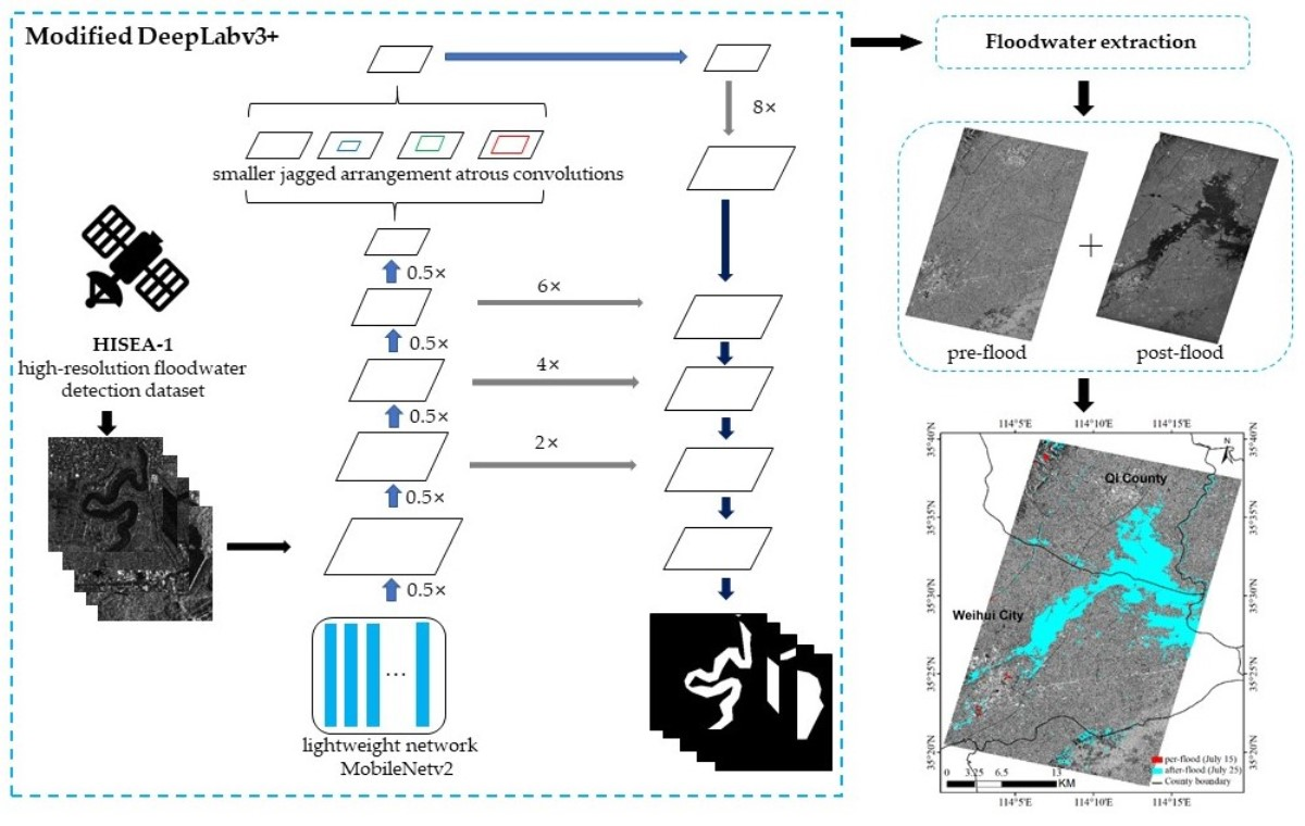
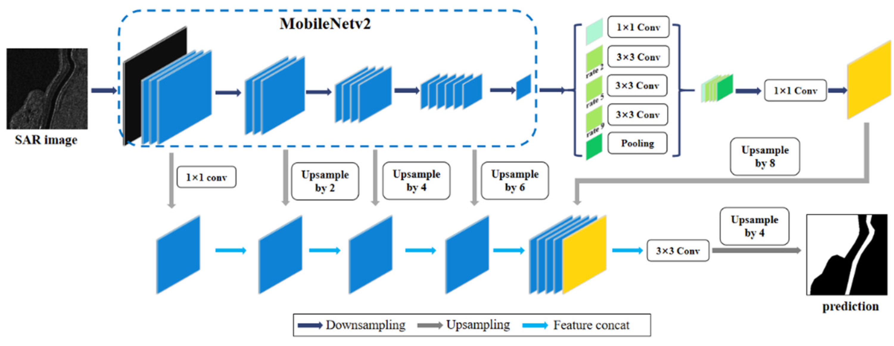
  • A Modified DeepLabv3+ Model is proposed to achieve accurate and fast extraction of floodwaters. The improvements include (1) using a lightweight network called MobileNetv2 as the backbone to improve floodwater detection efficiency, (2) employing small jagged arrangement atrous convolutions to capture features at small scales and improve pixels utilization, and (3) increasing the upsampling layers to refine the segmented boundaries of water bodies.
  • Two flooding events in China and the United States are analyzed to monitor the dynamic changes and flood levels of water bodies in the affected area.
The organization of this paper is as follows: Section 2 introduces the dataset production and label making process; Section 3 details the methodology for floodwater extraction, highlighting the improvements of Modified DeepLabv3+ model; Section 4 reports the main results, including model performance and validation; Section 5 is an analysis of two flooding events in China and the United States in July 2021; conclusions are given in Section 6.

2. Materials

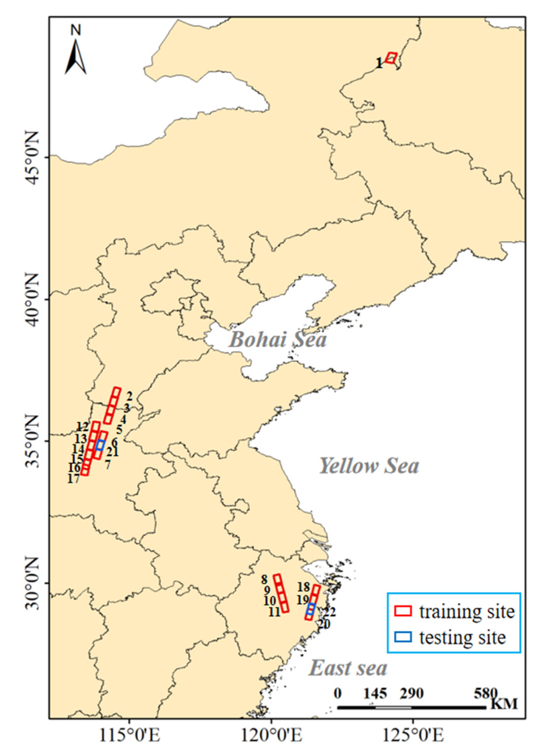
2.1. Water Body Extraction Images

In this work, we utilize HISEA-1 SAR images to train and test Modified DeepLabv3+ model for floodwater segmentation. HISEA-1 is a C-band SAR minisatellite with a weight of 185 kg and an incident angle range of 20°–35°. HISEA-1 operates in VV polarization and three different imaging modes ranging from 1 to 20 m resolution and 5 to 100 km swath width (see Xue et al. [27] for more details).
We selected 20 HISEA-1 images captured in 2021 to create the dataset for flood water extraction. These 20 images comprise three different flood events with their locations shown by the red box in Figure 1. All images are level 2 ORG (orthorectification geolocation) products, with striping mode, 3 m resolution, and VV polarization.
The first scene (Image No. 1 in Figure 1 and Table 2, hereafter) comes from the dam break event of Hulunbuir, Inner Mongolia. On 18 July 2021, the dams of Yong’an Reservoir and Xinfa Reservoir burst one after another after enduring continuous heavy rainfall, causing the G111 National Highway to be washed away and many roads to be interrupted.
Seven scenes (Image Nos. 8–11 and Nos. 18–20) are from the typhoon In-Fa flood event, taken on 25 July 2021 and 26 July 2021, respectively. Typhoon In-Fa was the sixth typhoon in 2021, landing in Zhoushan City and Jiaxing City, Zhejiang Province at approximately 12:30 a.m. on 25 July and 9:50 a.m. on 26 July, respectively. In-Fa was a slow-moving typhoon which brought strong winds and heavy rainfall to Ningbo, Shaoxing, Hangzhou, Jiaxing, and other places, causing flooding and waterlogging in many cities.
Lastly, 12 scenes (Image Nos. 2–7 and Nos. 12–17) are from a rare heavy rainstorm and flood event in Henan Province in July 2021. From 17 July 2021 to 23 July 2021, under the dual influence of the Western Pacific subtropical high and typhoon In-Fa, Henan encountered a historically exceptionally heavy rain, causing many rivers to flood. Daily rainfall of 20 national meteorological stations in the province exceeded the historical extreme value since their establishment, with strong convective weather also occurring in Hebei and other surrounding provinces. Images corresponding to these observed flooding conditions provided the 20 scenes used to create the floodwater dataset. The dataset, therefore, includes images of various conditions including the reservoir dam break, urban waterlogging, flooded villages and farmland, and other flooded areas.
In addition, two images (Image Nos. 21–22) that did not participate in the training and validation of the model were selected to verify the robustness and generalization ability of the model. The main parameters of all images are given in Table 2.

2.2. Image Preprocessing

The SAR images used in this study were all acquired in HISEA-1 strip imaging mode. They are standard level 2 SAR orthorectification geolocation (ORG) products with 3 × 3 m resolution, generated from level 1 single look complex (SLC) products via multi-look processing, geometric correction, radiation correction, and geographic resampling. Hence, only a 3 × 3 Lee filter is adopted here to suppress speckle noise in all images, and the smoothed SAR images are then input into an annotation tool for dataset generation.

2.3. Dataset Generation

Image annotation includes the following steps:
  • Employment of an online annotation tool LabelMe [28] to manually label water bodies and construct sample sets referring to the optical image at the same time.
  • Batch-convert all marked json files to png image format.
  • Due to limitations of graphics processing unit (GPU) capabilities, all samples were resized to 256 × 256 sub-images without overlapping parts.
All sample sets were randomly allocated in the ratio of 6:2:2, and divided into 1404 training sets, 468 validation sets, and 468 test sets (a total of 2340 experimental data). This dataset covers 20,000 square kilometers, and it contains rivers, tributaries, reservoirs, lakes and paddy fields. Figure 2 shows examples of water types contained in the HISEA-1 dataset. The dataset can be accessed via Zenodo (https://zenodo.org/record/7198950 (accessed on 14 October 2022)).

3. Methodology

DeepLabv3+ is a mainstream encoder/decoder semantic segmentation network, selecting Xception [29] as the backbone network to extract abstract and high-level semantic features. Feature maps obtained through the backbone are then pooled to extract the features of multiscale objects through atrous spatial pyramid pooling (ASPP). The decoder module draws on the idea of FCN feature fusion, and it uses the skip connection structure to fuse high-level and low-level features to refine object edge segmentation. In this section, we modify the DeepLabv3+ model to be more suitable for flood mapping according to the characteristics of water bodies.

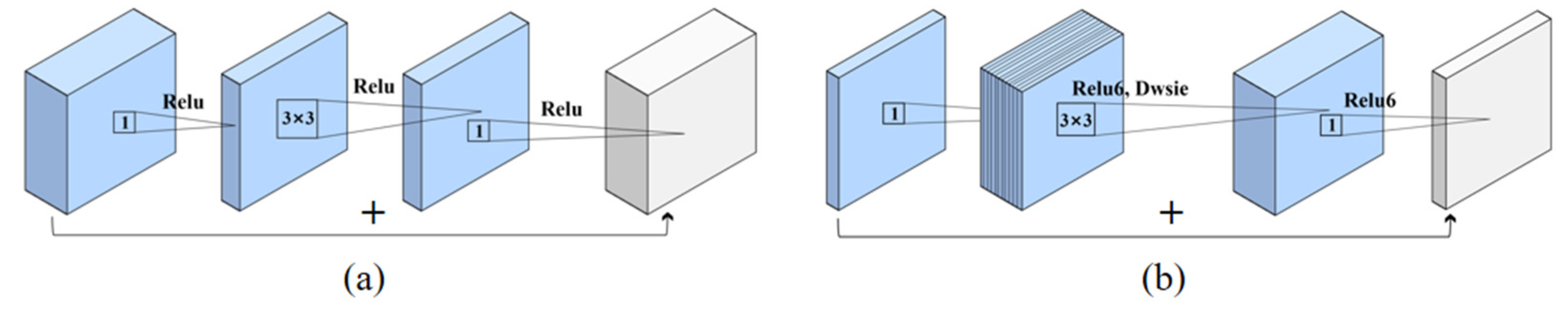
3.1. Using Lightweight Network MobileNetv2 as Encoder

Xception is an extreme Inception [30] module which changes the 1 × 1 convolution and the 3 × 3 convolution in Inception-v3 [31] into a unified 1 × 1 convolution operation, followed by a 3 × 3 convolution operation that fully decouples channel correlation and spatial correlation. Depthwise separable convolution is used to replace the convolution operation in this network. Xception contains a total of 36 convolutional layers and 14 modules with many parameters.
In order to more quickly and accurately extract flood water features, we modified the DeepLabv3+ to instead use the lightweight encoder MobileNetv2. MobileNetv2 is commonly used in mobile or embedded devices with fast responsiveness consisting of bottlenecks stacked by multiple inverse residual blocks and linear blocks stacked. The inverse residual block is inspired by the residual block in ResNet [32]. The residual block (Figure 3a) is narrow in the middle and wide on both sides. It first uses a 1 × 1 convolution kernel to drop the channel, and then connect the ReLU nonlinear activation. Next, it uses a 3 × 3 convolution and ReLU, as well as a 1 × 1 convolution and ReLU, to restore the number of feature map channels before adding them to the input. The inverse residual block (Figure 3b) is narrow on both sides and wide in the middle. First, it goes through a 1 × 1 convolution to increase the number of channels, and then uses 3 × 3 depthwise separable convolutions and ReLU6 to extract features. It finishes by using a 1 × 1 convolution to reduce the number of channels and adding it to the input. Overall, the number of feature map channels at both ends of the inverse residual block is very small. The total amount of computation is also greatly reduced due to the use of depthwise separable convolution. MobileNetv2 has two inverse residual block modules. The input and output dimensions of the convolution module with stride 1 are the same size, and the identity mapping structure is used. The size of the input and output of the convolution module with stride 2 is different, and the identity mapping structure is not used.
There are two primary differences between MobileNetv2 and Xception. First, the order of depthwise convolution and pointwise convolution is different. In MobileNetv2, the network first performs a 3 × 3 convolution on each channel, and then performs a 1 × 1 pointwise convolution. Xception performs a 1 × 1 convolution first, and then a 3 × 3 convolution operation. The second difference is that Xception uses ReLU for nonlinear activation after the 3 × 3 convolution operation, while MobileNetv2 performs inverted residuals. In the last layer of the block of MobileNetv2, a 1 × 1 convolution kernel is used to replace the ReLU nonlinear activation with linear activation to reduce the information loss caused by ReLU for features with fewer channels. MobileNetv2, therefore, has fewer parameters, is lighter, has a faster response, and is more conducive to water extraction.

3.2. Employing Smaller Jagged Arrangement Atrous Convolutions in ASPP

Inspired by the spatial pyramid pool [33], ASPP uses atrous convolution to sample the multiscale image feature at different rates. It consists of three parallel atrous convolutions of rates 6, 12, and 18, a 1 × 1 convolution, and global average pooling. However, it has been observed that such large atrous rates are better suited for large water body segmentation, making it difficult to capture smaller water bodies such as streams and ponds. Moreover, when there is a common factor relationship in an atrous rate group (e.g., 2, 4, and 8), there will be discontinuous feature information and low pixel utilization, also known as the “grid effect” [34]. We, therefore, change the atrous rate to 2, 5, and 9. The zigzag arrangement not only considers the segmentation requirements of large-scale and small-scale objects, but also effectively improves the utilization of pixels.

3.3. Adding More Upsampling Layers in Decoder

Since CNNs reduce feature map resolution and lose some detailed information during the pooling downsampling process, a skip connection structure was introduced in FCNs to improve model accuracy by combining deep features with low-level features. DeepLabv3+ adopts skip connection structures in the decoding module. In the upsampling layer, the features of two parts are fused: the first part is the shallow network feature obtained by down-channel processing the backbone network with a 1 × 1 size convolution kernel; the other part is the feature map output by ASPP after 1 × 1 convolution and four upsampling iterations. These two parts are fused and then subjected to 3 × 3 convolution and four upsampling iterations to obtain the prediction result. The encoder and decoder in DeepLabv3+ only have one connection, which allows the integration of shallow network features, but ignores deep semantic features and spatial information. This results in a good segmentation effect on clear images, but makes it difficult to obtain small-scale water body features and distinct outline information in remote sensing images.
Consequently, we added three upsampling layers in the decoder structure. More specifically, MobileNetv2 was divided into four blocks with each block consisting of three or four bottlenecks. The feature information upsampled from the previous feature map of the corresponding module in the encoder was then fused such that the information between the encoder and the decoder is more closely connected. This increased water outline clarity and feature details.

3.4. Modified DeepLabv3+ Model for Water Extraction

The architecture of Modified DeepLabv3+ is shown in Figure 4. The encoder module selects MobileNetv2 as the backbone network to extract abstract and high-level semantic features. The feature map obtained through the backbone network is then used to extract the features of multiscale objects through ASPP. The decoder uses the skip connection structure to construct four upsampling layers, fuses multilayer semantic features, refines object edge segmentation, and improves the accuracy of water extraction. The feature output by upsampling gathers the characteristic information of three branches. The first part is the low-level feature obtained by a 1 × 1 convolution dimensionality reduction operation of the backbone network MobileNetv2. The second is the output feature of the three newly added upsampling layers. The features in the encoder are subjected to two, four, and six iterations of bilinear interpolation upsampling to obtain the same resolution as the features in the lower layer. The third part is the feature map obtained by the combined features output by ASPP after 1 × 1 convolution dimension reduction and eight iterations of bilinear interpolation upsampling. The features of the three branches are fused and then undergo 3 × 3 convolution and four iterations of bilinear interpolation upsampling to recover the resolution of the feature map, and output the prediction results.

3.5. Metrics

The training model is quantitatively analyzed using three evaluation indicators: accuracy, F1, and intersection over union (IoU).
accuracy = TP + TN TP + TN + FP + FN .
precision = TP TP + FP .
recall = TP TP + FN .
F 1 = 2 × precision × recall precision + recall .
IoU = TP TP + FN + FP .
Accuracy refers to the proportion of all correctly classified pixels to the total pixels. F1 combines the results of precision and recall, allowing both to reach the highest value at the same time and be referenced as a harmonic average result. IoU refers to the ratio of the intersection and union between the ground truth and prediction, while the mIoU is the result of summing the intersection ratios of all categories and averaging them.
Since disaster monitoring has requirements for detection time, water extraction speed is also included in the evaluation scope in this paper. Detection rate refers to the time it takes for the model to test images. Higher image resolutions take more time.

4. Results

4.1. Experimental Setup

All experiments were carried out on a workstation with an Intel Xeon Gold 5118 Processor, 128 G RAM, and NVIDA Tesla V100-PCIE 32 GB graphics card using the PyTorch framework. We set the number of iterations for all training models to be 13 K, the training epoch to 300, and the initial learning rate to 0.001 with a ploy learning strategy. The momentum-based stochastic gradient descent method was used to optimize the network. The weight decay and momentum were set to 0.0005 and 0.9, respectively. The batch size was set to 32. All training networks were performed for multiple iterations until the maximum number of iterations was reached.

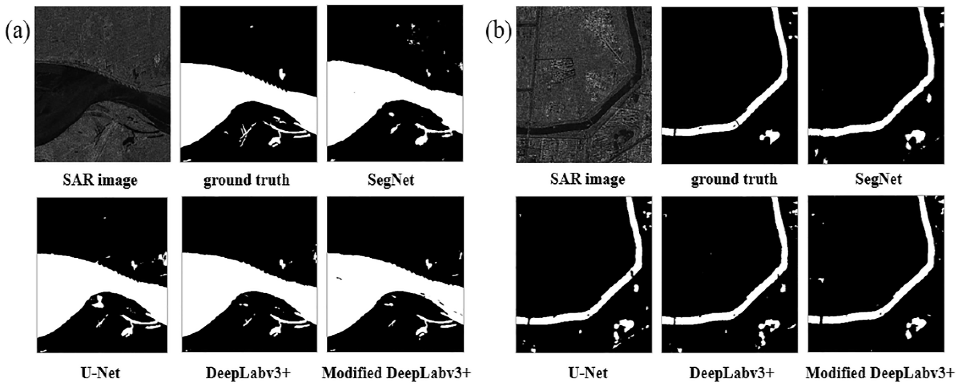
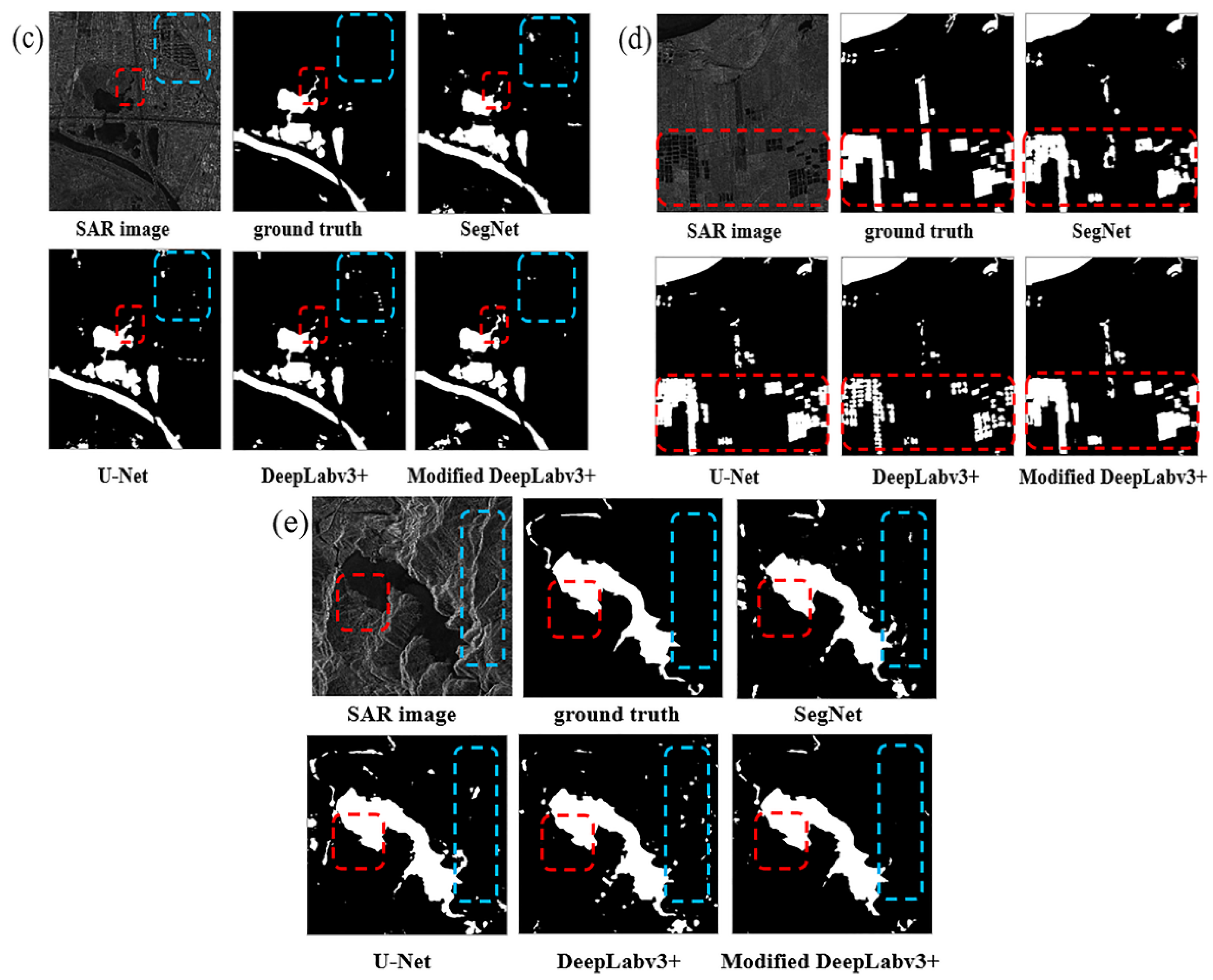
4.2. Comparison with Other Models

We compared the results of Modified DeepLabv3+ with U-Net, SegNet, and DeepLabv3+ to evaluate the performance of the modified model. Table 3 shows the model performance with respect to accuracy, F1, and mIoU. These results show that Modified DeepLabv3+ had the best segmentation accuracy and efficiency among the four models. Furthermore, it only took 46.8 s to extract all the water bodies in the testing set, which is 67% faster than the original DeepLabv3+ model.
Visual representation of results from the four model water body segmentations are shown in Figure 5. The large difference in results is reflected in the extraction of streams and paddy fields (Figure 5b,e). The streams and paddy fields extracted by the SegNet, U-Net, and DeepLabv3+ were discontinuous and incomplete, whereas Modified DeepLabv3+ could extract the complete water body. These segmentation results are highly consistent with the label water body, with clear contours and low false alarm rates. Additionally, DeepLabv3+ had a higher false alarm rate because it misidentified building and hill shadows near the lake as water bodies (Figure 5c,d). These results show that Modified DeepLabv3+ is an accurate and efficient water extraction model since the extracted water body features were complete with clear boundaries.

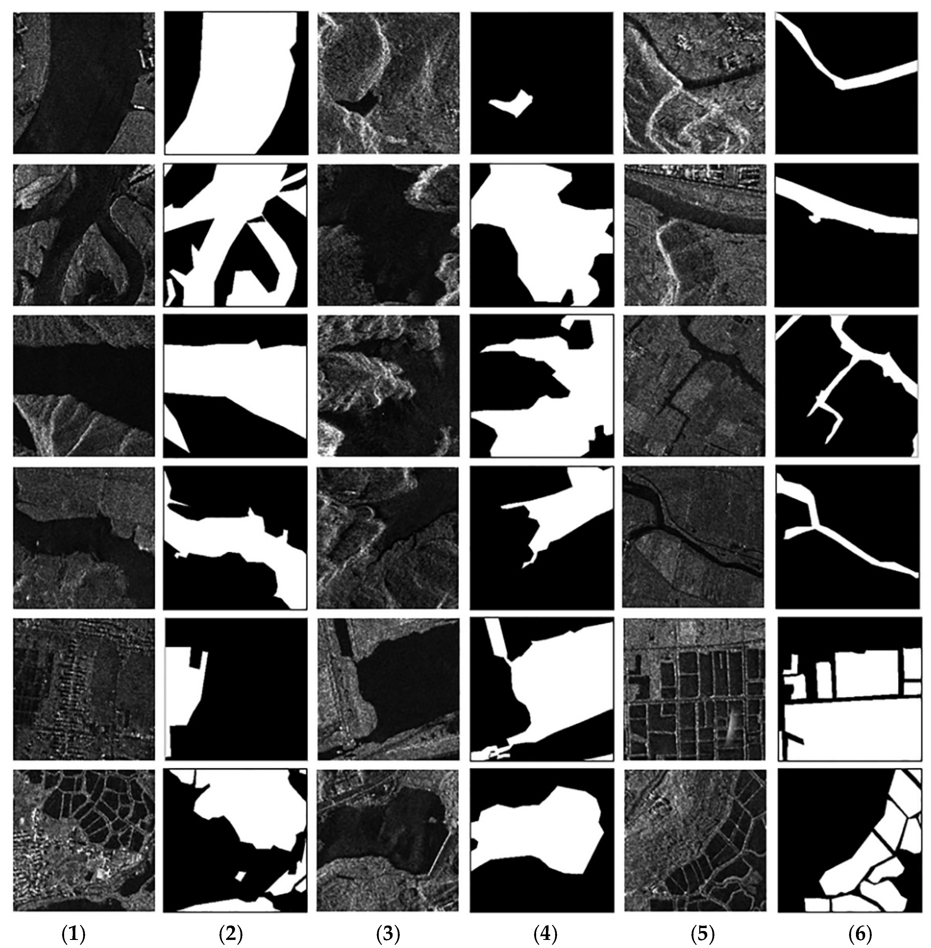
4.3. Performance for Various Water Body Types

To examine the robustness of the model, we selected SAR images (Image Nos. 21–22 in Figure 1 and Table 2) that did not participate in model training, verification, and testing. SegNet, U-Net, DeepLabv3+, and Modified DeepLabv3+ were used to segment images (all sized 1024 × 1024) of five different water body types: large rivers, tributaries, lakes, paddy fields, and reservoirs. The results are shown in Table 4. In terms of mIoU, SegNet, U-Net, and DeepLabv3+ showed little difference in the extraction test results of various water body types, with mIoUs of 89.84%, 90.90%, and 90.32%, respectively. On the other hand, the mIoU of the modified model reached 92.33%, and the segmentation effect was better than the other three models, proving its strong generalization ability. In terms of water body extraction efficiency, SegNet, U-Net, and DeepLabv3+ required 23.5 s, 24.5 s, and 25.5 s to detect the five specific scenes, respectively. In contrast, the proposed model only took 10.0 s.
Figure 6 shows a map of segmentation results for various water body types. All four models had better segmentation results in single, relatively regular water bodies, such as the extraction of river and stream water bodies. However, more prominent differences could be found in the detail for extracting irregular or dense water bodies. The first example is a narrow meandering stream extending from the lake (red box in Figure 6c). This meander was only identified by Modified DeepLabv3+. In general, farmland is the first to be affected when a flood occurs; thus, monitoring areas such as paddy fields is crucial for disaster assessment. When dense paddy fields were present within SAR imagery (red box in Figure 6d), Modified DeepLabv3+ had the best performance among the four models. Paddy fields captured by the proposed model were complete, coinciding with visual interpretations. For reservoirs, all four models could extract relatively complete reservoir shapes. However, since reservoirs are typically located in mountainous regions, shadows might interfere with model predictive capabilities since water bodies can have similar brightness values. This can make the boundary between water and shadow relatively blurry and complicate its extraction. Nevertheless, the results show that the target contour extracted by the modified model was clearer (red box in Figure 6e).
The blue boxes in Figure 6c,e show the result of the shaded area discrimination. The proposed model seldom misidentified shadows as water compared with the other three models. This means that it could effectively overcome the issues presented by the presence of shadows and accurately extract the water body information from a complex background.

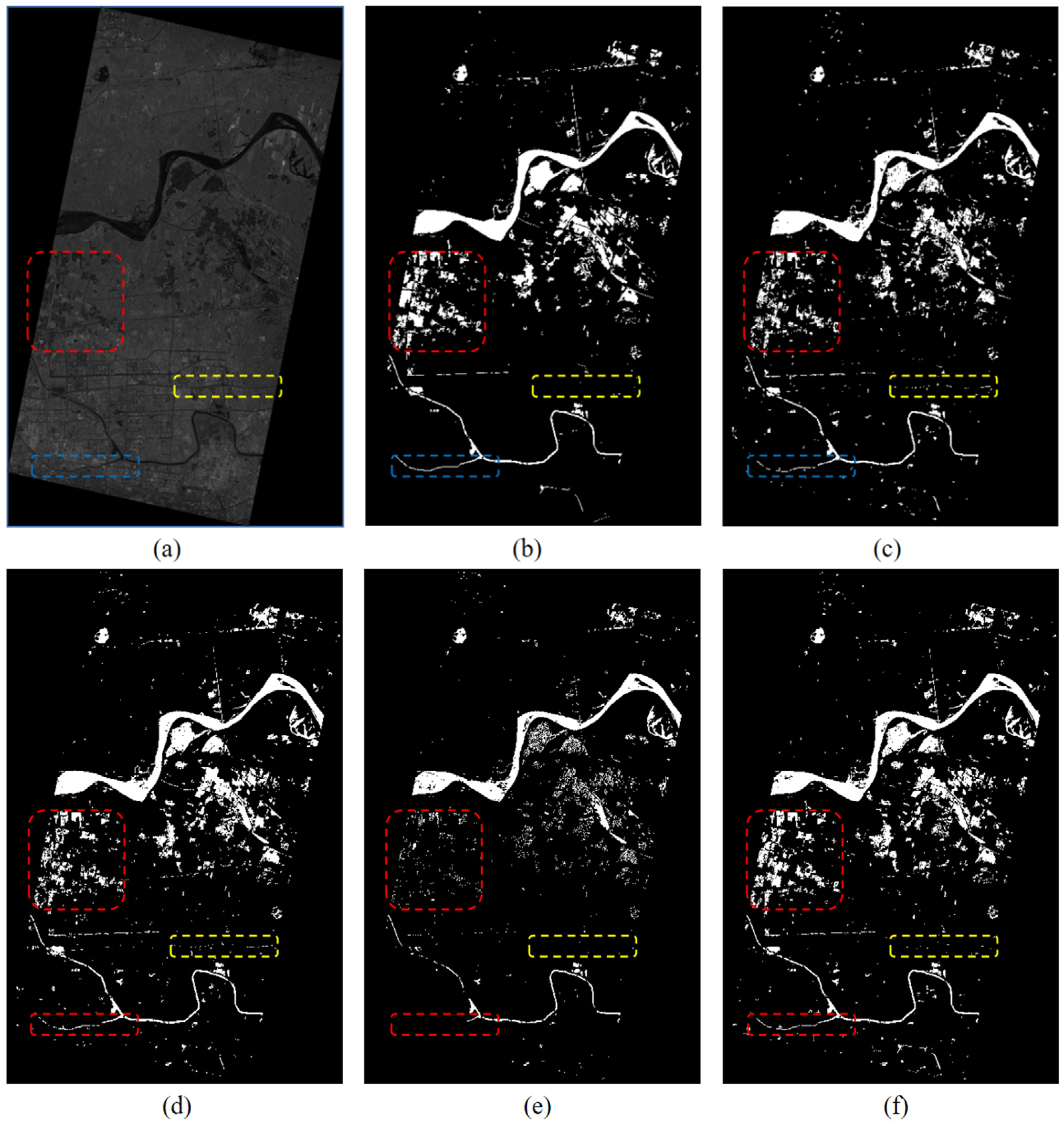
4.4. Performance for Large-Scale Floodwater Extraction

The impact of flood disasters is very wide, often causing large-scale inundation. This requires the segmentation algorithm to take into account large areas when performing water body extraction. Therefore, Modified DeepLabv3+ was applied to flood images of a heavy rainstorm flood event in Henan Province (Image No. 21 in Figure 1 and Table 2), which involved water bodies at a larger scale. The image denotes a flooded area with water bodies visually interpreted. This flood covered many water body types such as large rivers, lakes, streams, and paddy fields. There are multiple dense paddy fields below the Yellow River, roads in the urban center are complex and staggered, and small rivers are interspersed among them. This image also contained several small-scale water bodies, as well as building and mountain shadows.
The extracted results were post-processed by the open operation, and, after the morphological processing of first erosion and then expansion, the small protruding parts were removed, and the object contour was smoothed.
Table 5 summarizes the accuracy of each model for large-scale water detection. When applied to large-area water detection, the segmentation of the modified DeepLabv3+ resulted in accuracy, F1, and mIoU scores of 98.51%, 88.64%, and 89.01%, respectively. In contrast, mIoU from the original DeepLabv3+ model was 76.73%; thus, the modified model led to a 16% improvement. For detection efficiency, SegNet, U-Net, and DeepLabv3+ had similar detection times, taking more than 10 min to process a 9286 × 13,643 pixel SAR image respectively. The modified model required only 5 min to detect water bodies in a 1140 km2 image. Such efficient processing time is an indispensable advantage for real-time flood monitoring.
Figure 7 shows the visualization results of large-scale remote sensing image water extraction. According to the visual results, the extraction of water bodies in the Yellow River Basin were similar across the four models with the differences mainly reflected in the extraction of farmland and streams. Paddy fields are dense and numerous, making it increasingly difficult for model segmentation. Segmentation results of paddy fields (red box in Figure 7) indicate that the DeepLabv3 + model performed the worst since many paddy fields were not extracted. Furthermore, although SegNet and U-Net were able to extract a large amount of farmland information, this information was not complete. The paddy field segmentation result based on Modified DeepLabv3+ was complete and had higher coincidence with the visually interpreted results. For stream detection (blue box in Figure 7), the extraction results of SegNet and Modified DeepLabv3+ were more complete; but the streams extracted by SegNet had more fractures and the continuity was not as good as that of Modified DeepLabv3+. Roads can also serve as complications for water segmentation. Therefore, a highway was randomly selected to test the discrimination ability of the model. According to the results (yellow box in Figure 7), SegNet and U-Net had high false alarm rates, oftentimes classifying the expressway as water. The misclassification ratio of DeepLabv3+ to Modified DeepLabv3+ was lower.
On the basis of these factors, it can be concluded that Modified DeepLabv3+ can accurately, completely, and efficiently extract flood water bodies of various types, and it has a strong generalization ability and robustness.

5. Spatiotemporal Analysis of Two Flood Events

Furthermore, we took two severe flood events that were successfully captured by HISEA-1 as examples, and we used our new model to analyze the dynamic spatiotemporal changes of water bodies during the flood events.

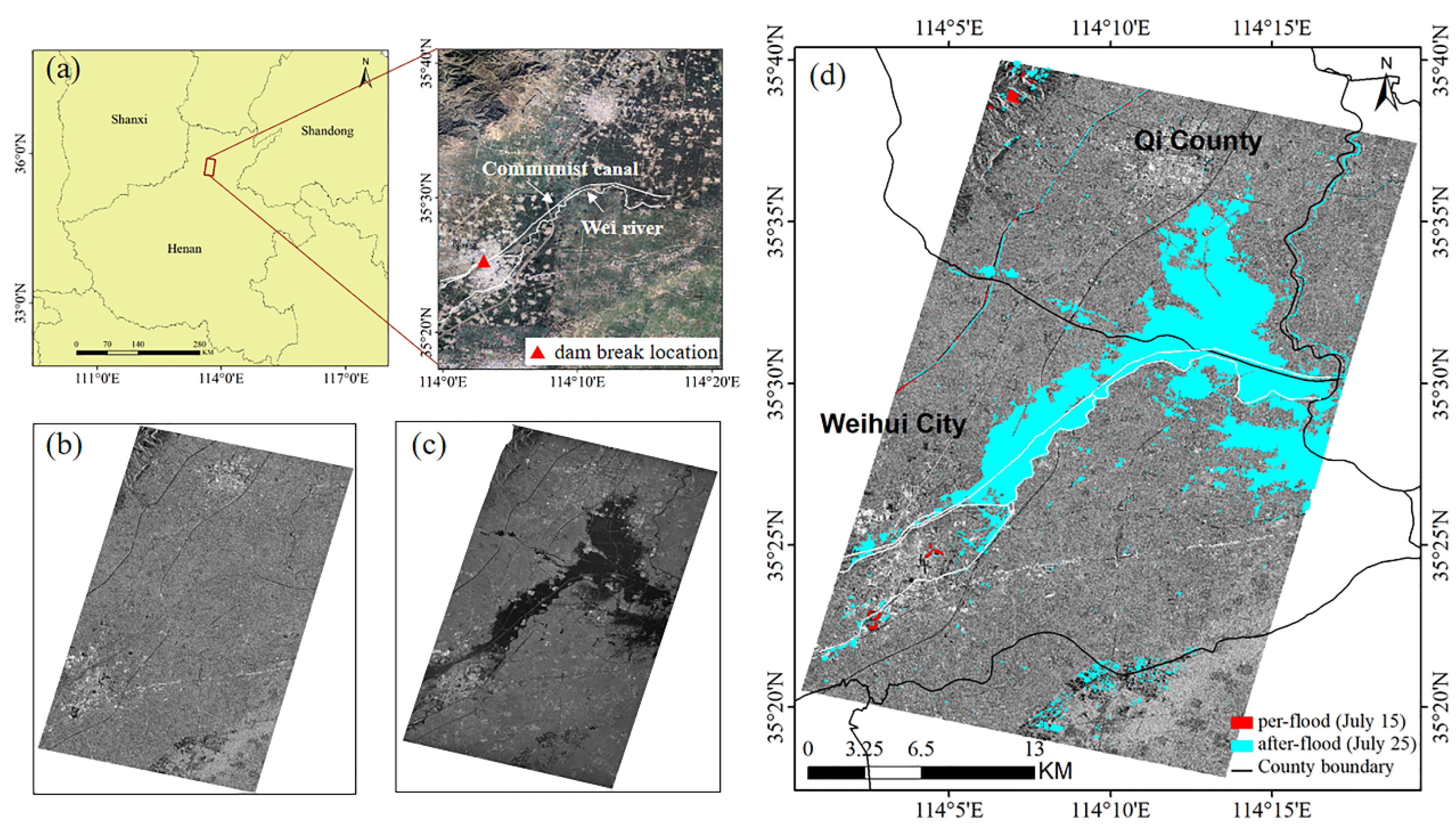
5.1. Severe Floods Caused by Extremely Heavy Rainfall in Henan Province, China

From 17 to 22 July 2021, Xinxiang City, Henan Province experienced the strongest extreme rainfall ever recorded, with a maximum rainfall of 907 mm. Affected by the continuous heavy rainfall and the concentrated discharge of upstream floods, the water level of the Communist Canal continued to rise, causing the dam to breach. The flood that overflowed the embankment poured into the Weihe River, resulting in severe flooding that affected Weihui City, Qi County, Huixian City, and other places.
We focus on the spatiotemporal distribution of floods in Wei River and Communist Canal, as well as the surrounding areas (see Figure 8a; central location of 35°29′N/114°9′E). Two SAR images with VV polarization were selected to monitor the floodwater change, including the pre-flood Sentinel-1 image in interferometric wide swath (IW) mode (acquired on 15 July 2021) and the post-flood HISEA-1 image in striping mode (acquired on 25 July 2021).
Figure 8d shows that the study area did not experience heavy rainfall during the pre-flood time period on 15 July. Only small water bodies such as rivers, paddy fields, and lakes were present before the disaster, with the total water area approximately 1.3 km2. On 25 July, after heavy rainfall, the flood area increased to 105.77 km2, accounting for 8.5% of the entire SAR image. The worst-hit areas of the river were at the junction of Weihui City and Qi Counties. The floods spilled out to the north and south, affecting many villages and farmland.

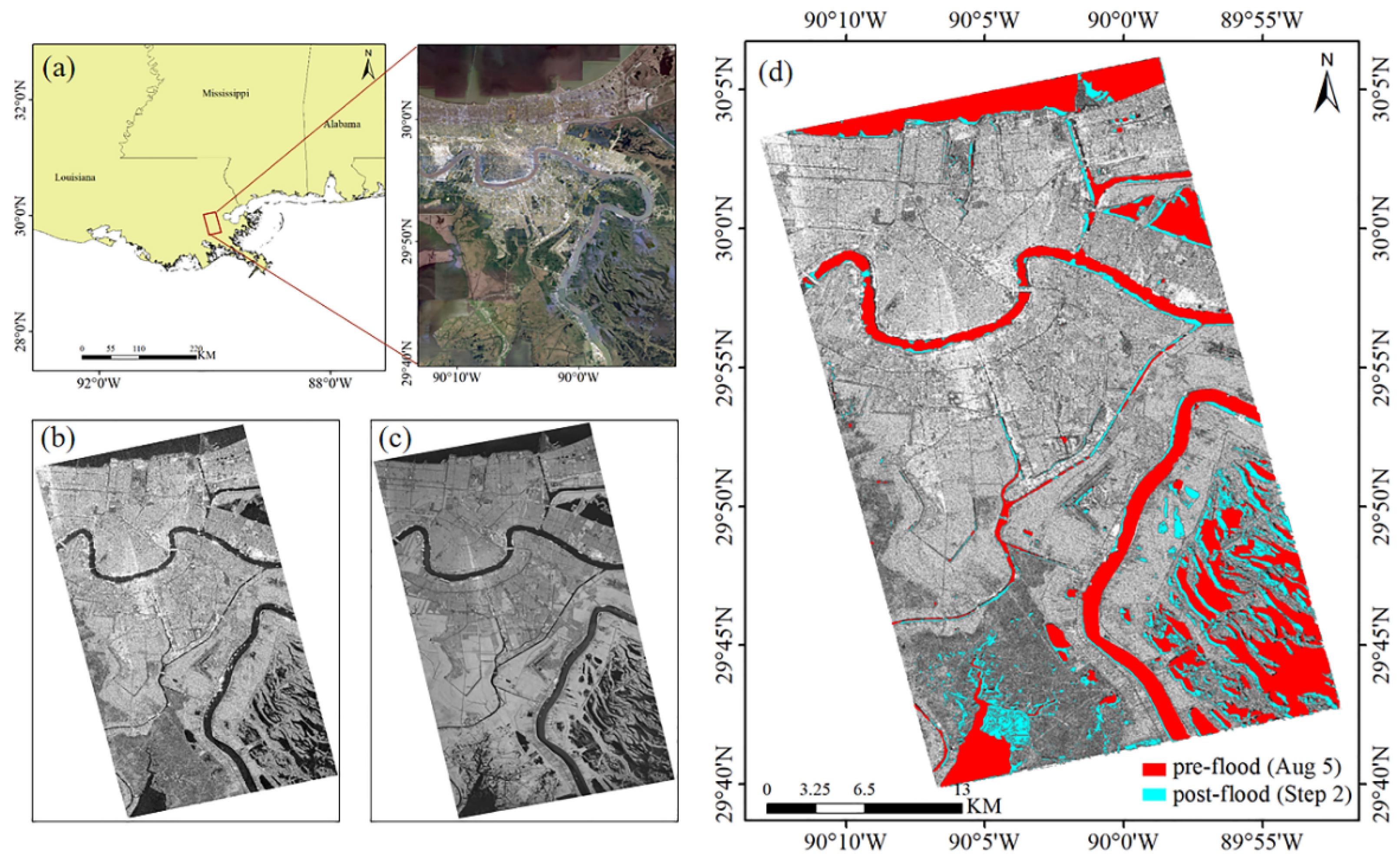
5.2. Flood Disaster Caused by Hurricane Ida in New Orleans, Louisiana, USA

On 29 August 2021, Category 4 Hurricane Ida made landfall in New Orleans, Louisiana, with winds of 209 kilometers per hour. Ida generated stormy conditions with heavy precipitation, leading to widespread inundation in New Orleans and knocking out power, toppling trees, and causing critical damage to bridges and roads.
The study area is shown in Figure 9a (central location of 29°52′N/90°02′E). We focused on changes in water bodies in the city center. Two SAR images with VV polarization were selected to monitor the floodwater change, including the pre-flood Sentinel-1 image in interferometric wide swath (IW) mode (acquired on 5 August 2021) and the post-flood HISEA-1 image in striping mode (acquired on 2 September 2021).
Results shown in Figure 9d indicate that most of the flooding occurred in the marsh and lake toward the south of the city. Floods poured into low-lying terrain, expanding the water bodies of swamps and lakes. The detected floodwaters on 2 September increased by 26.72 km2 compared to before the flood on 5 August.

6. Conclusions

Flooding events are nearly impossible to prevent; however, rapid and precise monitoring is important for their assessment and helping to mitigate potential damage. SAR is the ideal instrument for flood monitoring because it can provide all-weather and all-day observations since it is not limited by light conditions and cloud visibility like their optical counterparts. Flooding normally occurs as a consequence of heavy rainfall accompanied with high cloud coverage; thus, cloud penetration capabilities provide SAR satellites with unique advantages over other traditional satellites in flood monitoring. The flooding in New Orleans is a typical example of coastal flooding caused by extreme events such as hurricanes. Hurricanes can induce coastal flooding through various ways including heavy rainfall, storm surge, and levee breaches. The flooding that occurred in New Orleans after Hurricane Katrina in 2005 was attributed primarily to levee failures [35]. Most of the flooding that occurred was focused along the Mississippi River and the lakes near the southern coast, indicating that flooding was probably a result of both the heavy rainfall and storm surge. The flooding in Henan, China resulted from prolonged heavy rainfall; however, the causes of these heavy rainfalls are not yet fully understood. La Niña offers one possibility, since ENSO events can affect the East Asia Monsoon and consequently change local precipitation patterns [36].
In this paper, we proposed a robust and efficient deep learning model for flood mapping from HISEA-1 SAR imagery based on the DeepLabv3+ framework with three major modifications: (1) employing a lightweight MobileNetv2 as the DCNN’s backbone for rapid floodwater identification, (2) using ASPP with smaller dilation rates to adapt to diverse water body extraction and improve pixel utilization, and (3) increasing to three upsampling layers to fully integrate the features of the encoding and decoding structures and refine the water body contour boundary. The accuracy, F1, and mIoU of the modified model were 95.74%, 89.31%, and 87.79%, respectively, showing remarkable performance in flooding mapping compared to three models (U-Net, SegNet, and DeepLabv3+). Furthermore, Modified DeepLabv3+ is suitable for a multitude of water body types, especially for more difficult water extraction tasks of paddy fields and streams. The proposed model was then used to assess two severe flooding events in 2021 captured by the HISEA-1 SAR satellite. Results show that areas in Henan, China were severely affected by widespread flooding, leading to approximately 103.77 km2 of villages and farmland being inundated. New Orleans also experienced flooding as a result of Hurricane Ida, causing an inundation extent of nearly 26.72 km2. The exceptional performance of the model is in part due to the high-resolution imagery collected by the HISEA-1 SAR satellite, making both this satellite and this model extremely suitable for monitoring rapidly occurring disasters such as floods, as well as for observing the ocean and coastal regions.
As a supervised learning model, Modified DeepLabv3+ needs substantial training data. Here, we provide an open HISEA-1 SAR Floodwater Mapping Dataset in Zenodo; however, the water labels were generated manually and required a high human resource cost. Furthermore, the segmentation effect of Modified DeepLabv3+ may be limited by the accuracy and diversification of labels. If the training data have more diverse ground features, the model will have better segmentation results. Future work will extend the dataset to include more imagery from HISEA-1, as well as other high-resolution SAR satellites, and develop an automatic or semiautomatic labeling technique to improve the efficiency of annotation. DEM (digital elevation model) data could also be used to further improve the accuracy of floodwater segmentation, especially in mountainous areas.
Floodwater monitoring is a prominent task of emergency management, and SAR is a powerful tool in flood tracking due to its cloud-penetrating abilities. Here, we used HISEA-1 imagery to detect water bodies, demonstrating the potential of small SAR satellites in disaster monitoring. In the future, more low-cost SAR miniaturized satellites will be deployed to improve the emergency response time.

Author Contributions

Conceptualization, S.L.; writing—original draft preparation, S.L. writing—review and editing, L.M., X.G., X.-H.Y., D.E. and S.X.; visualization, S.L. All authors have read and agreed to the published version of the manuscript.

Funding

This research was supported by the National Key R&D Program of China (2019YFA0606702), the National Natural Science Foundation of China (91858202, 41630963, and 41776003) and the Industry–University Cooperation and Collaborative Education Projects (202102245034). D.E. and X.-H.Y. have been supported by NSF (IIS-2123264) and NASA (80NSSC20M0220).

Acknowledgments

The authors would like to thank all participants and collaborators involved in the HISEA-1 C-band SAR satellite project, such as Spacety, CETC 38th Institute and Fujian Tendering Purchasing Group Co., Ltd.

Conflicts of Interest

The authors declare no conflict of interest.

References

  1. Li, Y.; Zhao, S.-S. Floods losses and hazards in China from 2001 to 2020. Clim. Chang. Res. 2022, 18, 154–165. [Google Scholar] [CrossRef]
  2. Xia, J.; Wang, H.; Gan, Y.; Zhang, L. Research progress in forecasting methods of rainstorm and flood disaster in China. Torrential Rain Disasters 2019, 5, 416–421. [Google Scholar]
  3. Zaart, A.E.; Ziou, D.; Wang, S. Segmentation of SAR images. Pattern Recognit. 2002, 35, 713–724. [Google Scholar] [CrossRef]
  4. Liang, J.; Liu, D. A local thresholding approach to flood water delineation using Sentinel-1 SAR imagery. ISPRS J. Photogramm. Remote Sens. 2020, 159, 53–62. [Google Scholar] [CrossRef]
  5. Chini, M.; Hostache, R.; Giustarini, L.; Matgen, P. A Hierarchical Split-Based Approach for Parametric Thresholding of SAR Images: Flood Inundation as a Test Case. IEEE Trans. Geosci. Remote Sens. 2017, 55, 6975–6988. [Google Scholar] [CrossRef]
  6. Lang, F.; Yang, J.; Yan, S.; Qin, F. Superpixel Segmentation of Polarimetric Synthetic Aperture Radar (SAR) Images Based on Generalized Mean Shift. Remote Sens. 2018, 10, 1592. [Google Scholar] [CrossRef] [Green Version]
  7. Zhang, W.; Xiang, D.; Su, Y. Fast Multiscale Superpixel Segmentation for SAR Imagery. IEEE Geosci. Remote Sens. Lett. 2022, 19, 1–5. [Google Scholar] [CrossRef]
  8. Ijitona, B.; Ren, J.; Hwang, B. SAR Sea Ice Image Segmentation Using Watershed with Intensity-Based Region Merging. IEEE Int. Conf. Comput. Inf. Technol. 2014, 168–172. [Google Scholar] [CrossRef]
  9. Ciecholewski, M. River channel segmentation in polarimetric SAR images: Watershed transform combined with average contrast maximisation. Expert Syst. Appl. 2017, 82, 196–215. [Google Scholar] [CrossRef]
  10. Horritt, M.S.; Mason, D.C.; Luckman, A.J. Flood boundary delineation from Synthetic Aperture Radar imagery using a statistical active contour model. Int. J. Remote Sens. 2001, 22, 2489–2507. [Google Scholar] [CrossRef]
  11. Jin, R.; Yin, J.; Zhou, W.; Yang, J. Level Set Segmentation Algorithm for High-Resolution Polarimetric SAR Images Based on a Heterogeneous Clutter Model. IEEE J. Sel. Top. Appl. Earth Obs. Remote Sens. 2017, 10, 4565–4579. [Google Scholar] [CrossRef]
  12. Braga, M.; Marques, P.; Rodrigues, A.; Medeiros, S. A Median Regularized Level Set for Hierarchical Segmentation of SAR Images. IEEE Geosci. Remote Sens. Lett. 2017, 14, 1171–1175. [Google Scholar] [CrossRef]
  13. Pulvirenti, L.; Pierdicca, N.; Chini, M.; Guerriero, L. An algorithm for operational flood mapping from Synthetic Aperture Radar (SAR) data using fuzzy logic. Nat. Hazards Earth Syst. Sci. 2011, 2, 529–540. [Google Scholar] [CrossRef] [Green Version]
  14. Kuenzer, C.; Guo, H.; Schlegel, I.; Tuan, V.; Li, X.; Dech, S. Varying Scale and Capability of Envisat ASAR-WSM, TerraSAR-X Scansar and TerraSAR-X Stripmap Data to Assess Urban Flood Situations: A Case Study of the Mekong Delta in Can Tho Province. Remote Sens. 2013, 5, 5122–5142. [Google Scholar] [CrossRef] [Green Version]
  15. Inglada, J.; Mercier, G. A New Statistical Similarity Measure for Change Detection in Multitemporal SAR Images and Its Extension to Multiscale Change Analysis. IEEE Trans. Geosci. Remote Sens. 2007, 45, 1432–1445. [Google Scholar] [CrossRef] [Green Version]
  16. Long, S.; Fatoyinbo, T.E.; Policelli, F. Flood extent mapping for Namibia using change detection and thresholding with SAR. Environ. Res. Lett. 2014, 9, 206–222. [Google Scholar] [CrossRef]
  17. Clement, M.A.; Kilsby, C.G.; Moore, P. Multi-temporal synthetic aperture radar flood mapping using change detection. J. Flood Risk Manag. 2018, 11, 152–168. [Google Scholar] [CrossRef] [Green Version]
  18. Ronneberger, O.; Fischer, P.; Brox, T. U-Net: Convolutional Networks for Biomedical Image Segmentation. In Proceedings of the International Conference on Medical Image Computing and Computer-Assisted Intervention, Munich, Germany, 5–9 October 2015. [Google Scholar]
  19. Badrinarayanan, V.; Kendall, A.; Cipolla, R. SegNet: A Deep Convolutional Encoder-Decoder Architecture for Image Segmentation. IEEE Trans. Pattern Anal. Mach. Intell. 2017, 39, 2481–2495. [Google Scholar] [CrossRef]
  20. Chen, L.-C.; Papandreou, G.; Kokkinos, I.; Murphy, K.; Yuille, A.L. Semantic Image Segmentation with Deep Convolutional Nets and Fully Connected CRFs. In Proceedings of the International Conference on Learning Representations 2015, San Diego, CA, USA, 7–9 May 2015. [Google Scholar]
  21. Chen, L.-C.; Papandreou, G.; Kokkinos, I.; Murphy, K.; Yuille, A.L. DeepLab: Semantic image segmentation with deep convolutional nets, atrous convolution, and fully connected CRFs. IEEE Trans. Pattern Anal. Mach. Intell. 2018, 40, 834–848. [Google Scholar] [CrossRef] [Green Version]
  22. Chen, L.C.; Papandreou, G.; Schroff, F.; Adam, H. Rethinking Atrous Convolution for Semantic Image Segmentation. Preprint arXiv 2017, arXiv:1706.05587. [Google Scholar]
  23. Chen, L.C.; Zhu, Y.; Papandreou, G.; Schroff, F.; Adam, H. Encoder-Decoder with Atrous Separable Convolution for Semantic Image Segmentation; Springer: Cham, Switzerland, 2018. [Google Scholar]
  24. Kang, W.; Xiang, Y.; Wang, F.; Wan, L.; You, H. Flood Detection in Gaofen-3 SAR Images via Fully Convolutional Networks. Sensors 2018, 18, 2915. [Google Scholar] [CrossRef] [PubMed] [Green Version]
  25. Nemni, E.; Bullock, J.; Belabbes, S.; Bromley, L. Fully Convolutional Neural Network for Rapid Flood Segmentation in Synthetic Aperture Radar Imagery. Remote Sens. 2020, 12, 2532. [Google Scholar] [CrossRef]
  26. Bai, Y.; Wu, W.; Yang, Z.; Yu, J.; Zhao, B.; Liu, X.; Yang, H.; Mas, E.; Koshimura, S. Enhancement of Detecting Permanent Water and Temporary Water in Flood Disasters by Fusing Sentinel-1 and Sentinel-2 Imagery Using Deep Learning Algorithms: Demonstration of Sen1Floods11 Benchmark Datasets. Remote Sens. 2021, 13, 2220. [Google Scholar] [CrossRef]
  27. Xue, S.; Geng, X.; Meng, L.; Xie, T.; Huang, L.; Yan, X.-H. HISEA-1: The First C-Band SAR Miniaturized Satellite for Ocean and Coastal Observation. Remote Sens. 2021, 13, 2076. [Google Scholar] [CrossRef]
  28. Torralba, A.; Russell, B.C.; Yuen, J. LabelMe: Online Image Annotation and Applications. Proc. IEEE 2010, 98, 1467–1484. [Google Scholar] [CrossRef]
  29. Chollet, F. Xception: Deep Learning with Depthwise Separable Convolutions. In Proceedings of the 2017 IEEE Conference on Computer Vision and Pattern Recognition (CVPR), Honolulu, HI, USA, 21–26 July 2017. [Google Scholar]
  30. Szegedy, C.; Liu, W.; Jia, Y.; Sermanet, P.; Reed, S.; Anguelov, D.; Erhan, D.; Vanhoucke, V.; Rabinovich, A. Going Deeper with Convolutions. In Proceedings of the 2015 IEEE Conference on Computer Vision and Pattern Recognition (CVPR), Boston, MA, USA, 7–12 June 2015; pp. 1–9. [Google Scholar] [CrossRef] [Green Version]
  31. Szegedy, C.; Vanhoucke, V.; Ioffe, S.; Shlens, J.; Wojna, Z. Rethinking the Inception Architecture for Computer Vision. In Proceedings of the 2016 IEEE Conference on Computer Vision and Pattern Recognition (CVPR), Las Vegas, NV, USA, 27–30 June 2016; pp. 2818–2826. [Google Scholar] [CrossRef] [Green Version]
  32. He, K.; Zhang, X.; Ren, S.; Sun, J. Deep Residual Learning for Image Recognition. In Proceedings of the 2016 IEEE Conference on Computer Vision and Pattern Recognition (CVPR), Las Vegas, NV, USA, 27–30 June 2016; pp. 770–778. [Google Scholar] [CrossRef] [Green Version]
  33. He, K.; Zhang, X.; Ren, S.; Sun, J. Spatial Pyramid Pooling in Deep Convolutional Networks for Visual Recognition. IEEE Trans. Pattern Anal. Mach. Intell. 2015, 37, 1904–1916. [Google Scholar] [CrossRef] [Green Version]
  34. Wang, P.Q.; Chen, P.F.; Yuan, Y.; Liu, D.; Huang, Z.H.; Hou, X.D.; Cottrell, G. Understanding Convolution for Semantic Segmentation. In Proceedings of the 2018 IEEE Winter Conference on Applications of Computer Vision (WACV 2018), Lake Tahoe, NV, USA, 12–15 March 2018; pp. 1451–1460. [Google Scholar] [CrossRef] [Green Version]
  35. Pistrika, A.K.; Jonkman, S.N. Damage to residential buildings due to flooding of New Orleans after hurricane Katrina. Nat. Hazards 2010, 54, 413–434. [Google Scholar] [CrossRef]
  36. Zhang, W.; Jin, F.F.; Stuecker, M.F.; Wittenberg, A.T.; Timmermann, A.; Ren, H.L.; Kug, J.S.; Cai, W.; Cane, M. Unraveling El Nino’s impact on the East Asian Monsoon and Yangtze River summer flooding. Geophys. Res. Lett. 2016, 43, 11375–11382. [Google Scholar] [CrossRef]
Figure 1. Spatial distribution of training (red) and test (blue) sites.
Remotesensing 14 05504 g001
Figure 2. Examples of the HISEA-1 water body extraction dataset, including five common water types (rivers, reservoirs, streams, paddy fields, and lakes) and their corresponding ground truth. Columns (1), (3), and (5) are SAR images, while columns (2), (4) and (6) are the corresponding ground truth.
Remotesensing 14 05504 g002
Figure 3. (a) Residual block and (b) inverted residual block. 1: 1 × 1 convolution kernel, 3 × 3: 3 × 3 convolution kernel, Relu: ReLU nonlinear activation, Relu6: ReLU6 nonlinear activation, Dwise: depthwise convolution.
Remotesensing 14 05504 g003
Figure 4. The architecture of Modified DeepLabv3+.
Remotesensing 14 05504 g004
Figure 5. Visualization of water body segmentation for the four models: SegNet, U-Net, DeepLabv3+, and Modified DeepLabv3+. Water body types: (a) river, (b) stream, (c) lake, (d) reservoir, and (e,f) paddy field.
Remotesensing 14 05504 g005
Figure 6. Visualized results for extracting five different typical types of water bodies using four models: SegNet, U-Net, DeepLabv3+, and Modified DeepLabv3+. Water body types: (a) river, (b) stream, (c) lake, (d) paddy field, and (e) reservoir. The red and blue dashed boxes denote some typical comparative areas.
Remotesensing 14 05504 g006aRemotesensing 14 05504 g006b
Figure 7. Performance of four models for segmenting flood disaster: (a) flood disaster image of HISEA-1; (b) ground truth; extraction results from model (c) SegNet, (d) U-Net, (e) DeepLabv3+, and (f) Modified DeepLabv3+. The red, yellow, and blue dashed boxes denote some typical comparative areas.
Remotesensing 14 05504 g007
Figure 8. Geospatial analysis of severe floods in Henan Province in July 2021: (a) study area of flood event; (b) pre-flood SAR image with Sentinel-1; (c) post-flood image with HISEA-1; (d) floodwater monitoring thematic map with Modified DeepLabv3+ (red is pre-flood area on 15 July 2021; cyan is post-flood area on 25 July 2021).
Remotesensing 14 05504 g008
Figure 9. Flood mapping based on Modified DeepLabv3+ caused by Hurricane Ida in New Orleans: (a) study area; (b) pre-flood SAR image with Sentinel-1 on 5 August 2021; (c) post-flood SAR image with HISEA-1 on 2 September 2021; (d) flood monitoring thematic map with Modified DeepLabv3+ (red is pre-flood area on 5 August 2021, cyan is post-flood area on 2 September 2021.
Remotesensing 14 05504 g009
Table 1. Comparison of various SAR image segmentation techniques.
Segmentation TechniquesCharacteristic, AdvantageLimitation, Disadvantage
Threshold-basedLow computation complexity; no need for prior knowledgeSpatial details are not considered; not good if no clear peaks
Superpixel-basedGroups of pixels that look similarChallenging in detailed information and superpixel number
Watershed-basedRegion-based; detected boundaries are continuousComplex calculation of gradients; over-segmentation
Active contour methodsGood performance for complicated boundariesDependent on initial contour
Classification-based Pixel-level classification; more choice of classification methodsDependent on classifying effect; some models need to be trained
Table 2. HISEA-1 images used in the construction of floodwater extraction dataset, including the location, acquisition time, orbit direction, incidence angle in the mid-swath, and size of the images.
Image IDTime DateCentral LocationStudy AreaOrbit DirectionIncidence Angle Mid-SwathImage Size
Training region
No. 121 July 202148°30′N/124°12′EInner MongoliaDescending24.5°9819 × 13,833
No. 225 July 202136°42′N/114°31′EHebeiDescending28.5°9926 × 13,862
No. 325 July 202136°24′N/114°26′EHebeiDescending28.5°9924 × 13,863
No. 425 July 202136°6′N/114°20′EHenanDescending28.5°9921 × 13,863
No. 525 July 202135°47′N/114°15′EHenanDescending28.5°9917 × 13,862
No. 625 July 202135°10′N/114°3′EHenanDescending28.5°9918 × 13,863
No. 725 July 202134°34′N/113°53′EHenanDescending28.5°9286 × 13,640
No. 825 July 202130°7′N/120°12′EZhejiangAscending26.5°9487 × 14,504
No. 925 July 202129°49′N/120°17′EZhejiangAscending26.5°9476 × 14,503
No. 1025 July 202129°30′N/120°30′EZhejiangAscending26.5°9471 × 14,501
No. 1125 July 202129°9′N/120°27′EZhejiangAscending26.5°9482 × 14,502
No. 1226 July 202135°29′N/113°48′EHenanDescending16.25°9157 × 14,163
No. 1326 July 202135°11′N/113°43′EHenanDescending16.25°9202 × 14,174
No. 1426 July 202134°50′N/113°38′EHenanDescending16.25°9199 × 14,176
No. 1526 July 202134°31′N/113°34′EHenanDescending16.25°9175 × 14,174
No. 1626 July 202134°12′N/113°29′EHenanDescending16.25°9183 × 14,177
No. 1726 July 202133°59′N/113°26′EHenanDescending16.25°9200 × 14,196
No. 1827 July 202129°45′N/121°34′EZhejiangDescending29.5°9856 × 14,508
No. 1927 July 202129°25′N/121°28′EZhejiangDescending29.5°9856 × 14,508
No. 2027 July 202128°54′N/121°20′EZhejiangDescending29.5°9842 × 14,506
Testing region
No. 2125 July 202134°51′N/113°58′EHenanDescending28.5°9286 × 13,643
No. 2227 July 202129°6′N/121°23′EZhejiangDescending29.5°9833 × 14,502
Table 3. Performance of four models, with the best results for each metric shown in bold.
ModelsAccuracyF1mIoUDetection Time (s)
SegNet0.94470.86030.8441187.2
U-Net0.95170.88010.8636140.4
DeepLabv3+0.94270.85510.8390140.0
Modified DeepLabv3+0.95740.89360.877946.8
Table 4. Performance of four models for extracting five typical water bodies from SAR image, the best ones for are in bold.
ModelsAccuracyF1mIoUDetection Time (s)
SegNet0.97500.90350.898423.5
U-Net0.97770.91480.909024.5
DeepLabv3+0.97650.90680.903225.5
Modified DeepLabv3+0.98200.92830.937610
Table 5. Performance of four models for floodwater extraction from a large-scale SAR, with the best results shown in bold.
ModelsAccuracyF1mIoUDetection Time (min)
SegNet0.98070.84930.858910.5
U-Net0.98320.87200.877610.4
DeepLabv3+0.97100.72180.767310.3
Modified DeepLabv3+0.98510.88640.89014.9
Note: This is the entire SAR image, with a size of 9286 × 13,643.
Publisher’s Note: MDPI stays neutral with regard to jurisdictional claims in published maps and institutional affiliations.

