Article

DP–MHT–TBD: A Dynamic Programming and Multiple Hypothesis Testing-Based Infrared Dim Point Target Detection Algorithm

1
National Key Laboratory of Science and Technology on Automatic Target Recognition, College of Electronic Science and Technology, National University of Defense Technology, Changsha 410073, China
2
Department of Military Education, College of Military Basic Education, National University of Defense Technology, Changsha 410073, China
*
Author to whom correspondence should be addressed.
Remote Sens. 2022, 14(20), 5072; https://doi.org/10.3390/rs14205072
Submission received: 19 August 2022 / Revised: 1 October 2022 / Accepted: 8 October 2022 / Published: 11 October 2022

Abstract

:
The detection and tracking of small targets under low signal-to-clutter ratio (SCR) has been a challenging task for infrared search and track (IRST) systems. Track-before-detect (TBD) is a widely-known algorithm which can solve this problem. However, huge computation costs and storage requirements limit its application. To address these issues, a dynamic programming (DP) and multiple hypothesis testing (MHT)-based infrared dim point target detection algorithm (DP–MHT–TBD) is proposed. It consists of three parts. (1) For each pixel in current frame, the second power optimal merit function-based DP is designed and performed in eight search areas to find the target search area that contains the real target trajectory. (2) In the target search area, the parallel MHT model is designed to save the tree-structured trajectory space, and a two-stage strategy is designed to mitigate the contradiction between the redundant trajectories and the requirements of more trajectories under low SCR. After constant false alarm segmentation of the energy accumulation map, the preliminary candidate points can be obtained. (3) The target tracking method is designed to eliminate false alarms. In this work, an efficient second power optimal merit function-based DP is designed to find the target search area for each pixel, which greatly reduces the trajectory search space. A two-stage MHT model, in which pruning for the tree-structured trajectory space is avoided and all trajectories can be processed in parallel, is designed to further reduce the hypothesis space exponentially. This model greatly reduces computational complexity and saves storage space, improving the engineering application of the TBD method. The DP–MHT–TBD not only takes advantage of the small computation amount of DP and high accuracy of an exhaustive search but also utilizes a novel structure. It can detect a single infrared point target when the SCR is 1.5 with detection probability above 90% and a false alarm rate below 0.01%.

1. Introduction

Target detection techniques in infrared (IR) images have played an important role in military and civil applications. IR imaging of long-range space targets, which can be modeled as point targets, contain little information about shape and texture. These point targets are usually buried in strong clutter. Therefore, detecting dim small IR targets remains a challenging problem [1,2,3,4]. During the past few decades, scholars have performed many studies on dim small-target detection. Existing IR small-target detection methods can be roughly divided into three categories: TBD methods, detect-before-track (DBT) methods and deep learning (DL)-based methods.
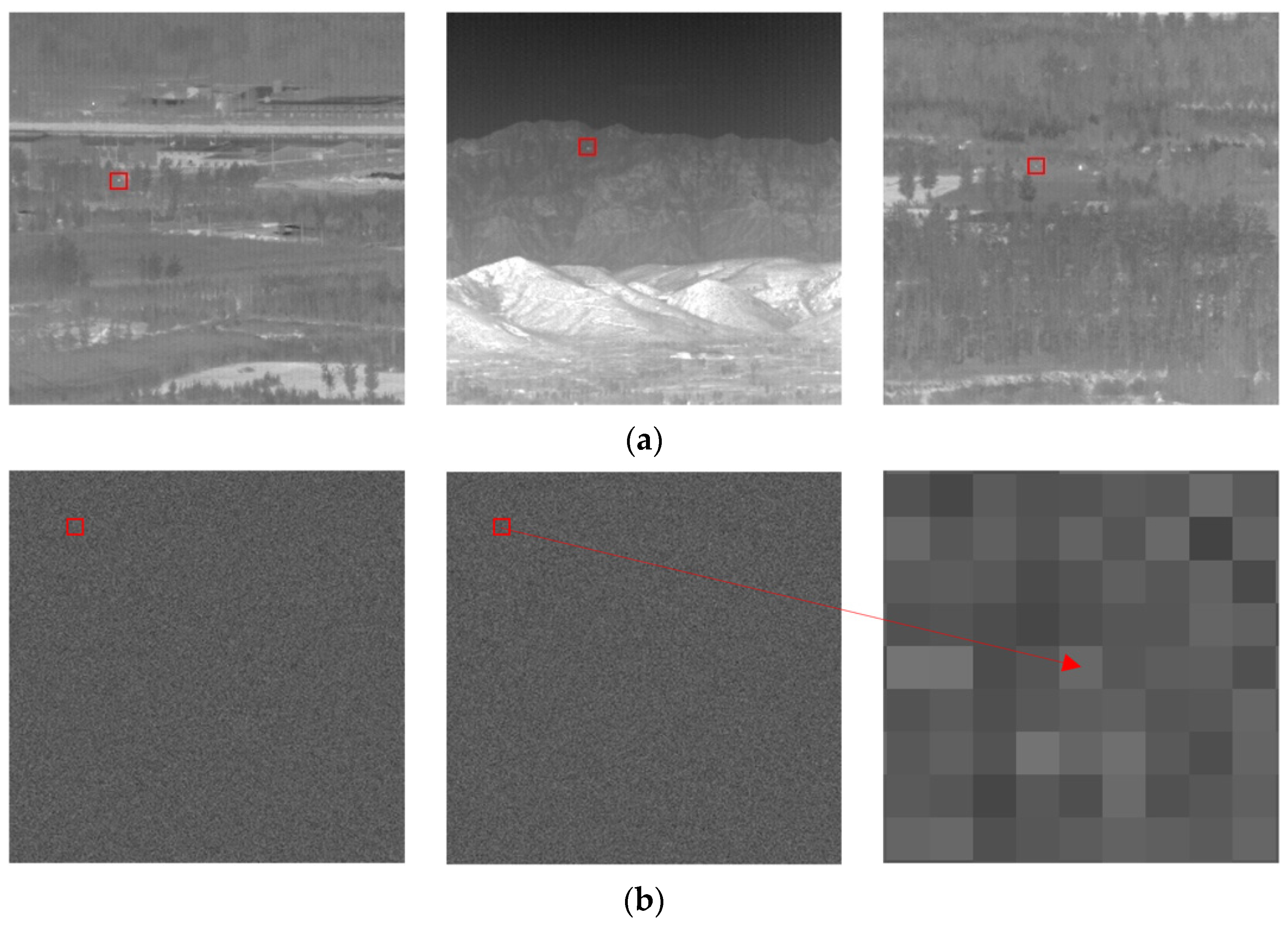
All methods have advantages and disadvantages. DBT methods, such as the classical local contrast measure (LCM) [5], local intensity and gradient (LIG) [6] and IR patch-image model (IPI) [7], concentrate on detecting targets in a single frame based on prior information. These methods are usually based on the image data structure and are designed to enhance the target, suppress the background, expand the contrast between the target and the background to improve the recognizability of the target, and then realize the detection of the target. Generally, this kind of method has the advantages of low complexity, high efficiency and easy hardware implementation. However, when the target SCR is low (SCR 1.5), many false alarms are produced, and the detection accuracy is decreased. Under low SCR conditions, TBD methods, such as 3-D matched filtering [8], Hough transform (HT) [9,10,11], DP [12] and MHT [13], are more stable and demonstrate better detection performance because they usually utilize spatial and temporal information by capturing the target trajectory. However, the computational cost and storage requirements of this kind of method inevitably increase, making practical applications difficult. Recently, DL methods, such as the single shot multibox detector (SSD) [14], you only look once (YOLO) [15], and Faster-RCNN [16], have already achieved remarkable progress in the target detection field. Relying on their strong feature extraction and generalization ability, neural network-based infrared target detection methods, such as the spatial–temporal feature-based detection framework [1], target-oriented shallow–deep feature (TSDF)-based detection method [2] and TBC-Net [17], have attracted increasing attention. In the previous work [1,2], some DL-based IR target detection algorithms were analyzed in detail. When the target has certain shape or texture information (size greater than 2 × 2) and the characteristics of background clutter are spatially nonstationary but temporally stationary, as with the images in Figure 1a, DL methods could play a role in the IR target detection field by assisting some techniques, such as shallow–deep feature fusion, spatial–temporal information extraction, and a reasonable sample selection strategy. However, when the target occupies only one pixel and the background clutter is temporally nonstationary, as with the images in Figure 1b, it is difficult for the DBT and DL methods to detect targets mainly for the following reasons. (1) Because the target SCR is very low, there are many pixels similar to the target in a single frame image, and the contrast between the target and the background is very low. Even the human eye cannot distinguish the target from the background by relying only on gray information. (2) The spatial–temporal information extraction method applied to the temporally stationary background has difficulty playing a role in the temporally nonstationary background, resulting in the neural network not learning the useful features. Taking the spatial–temporal information extraction method in [2] as an example, to suppress the background and extract the moving features of the target, the operations of frame subtraction and addition are used. When applied to an infrared sequence with a temporally nonstationary background, this kind of operation will not suppress the background but will reduce the SCR of the target and increase the difficulty of detection. This work focuses on the dim point target detection task. The problem analysis, methods and experiment part in this work focus on the 1 × 1 point target. The key to solving the problem of infrared point target detection under low SCR conditions is to adopt an appropriate TBD method; that is, first accumulate the energy of the target along the target trajectory to improve the SCR, and then detect the target.
In recent years, DP-TBD has become a hot research direction. The core idea of DP is to transform a complex multistep decision process into multiple single-stage decision processes and then optimize each decision to obtain a global optimal solution. The algorithm has clear principles, and the operation is based on the pixel level. This method is relatively small in computation and storage and easy to implement in hardware. There have been several improved DP-TBD methods in recent years. Direction information-based DP methods [18,19,20] have been proposed to reduce the number of pseudo trajectories under a strong clutter background and reduce the search range to decrease the diffusion effect of the target energy in the accumulation process. As the coverage of the target maneuvering range is limited to the fixed transition step, ISTS⁃DP⁃TBD (TBD algorithm with an improved state transition set) [21] was proposed. The state search efficiency of the maneuvering target is improved with optimization of the state transition strategy. PC-DP-TBD (DP-TBD method using parallel computing) [22] was proposed to solve the problem that the adjacent targets may interfere with each other and the computational complexity is increased with the number of targets. Although some progress has been made in DP-TBD, there are several problems to be solved [23,24]:
(1) The algorithm is affected by some parameters, such as the number of state transitions, the number of accumulation frames and the type of merit function value function. The selection of parameters has a great impact on the performance of the algorithm. It is difficult to find a set of parameters that is suitable for different backgrounds.
(2) Agglomeration effect. When tracking and detecting a target, the energy is accumulated along the possible trajectories. After K frame accumulation, the merit value of the target state increases, and in most cases this value is the largest. However, during the accumulation process, the energy of the target in the previous observation frame will diffuse to the next observation frame, forming a cluster of observation areas with similar energy. This is also known as the ‘agglomeration effect’. This effect becomes increasingly serious with increasing accumulation frames. When the SCR is low, after accumulation, the agglomeration effect will occur not only in the target but also in noise with strong energy, and even the diffusion of noise will be greater than that of the target. In this case, the state of this kind of noise is stronger than that of the target, which is not conducive to target detection or tracking. In addition, when there are multiple adjacent targets, there will be many trajectories with similar energy after energy accumulation. At this time, the agglomeration areas of different targets may overlap, causing difficulties in differentiating different targets. This is also the reason why most algorithms require the targets to be neither adjacent nor intersected.
Due to the above problems, compared with exhaustive search methods, the DP-TBD method performance can be reduced by 3 dB [12]. When the energy of the detected target drops to a certain extent, even if the number of accumulated observation frames is increased, the detection performance is poor. Even for some improved methods [21,25,26,27], the detection performance will be greatly reduced when the SCR is lower than 1.8.
Therefore, to achieve high-precision point target detection under low SCR (SCR 1.5), an exhaustive search method needs to be adopted. The real target trajectory can be found by searching as many trajectories as possible. The classical representative algorithm is MHT. However, the number of trajectories increases exponentially with the number of accumulation frames, causing tremendous computation and storage costs, so it is difficult to realize the accumulation of many frames. Therefore, the key to exhaustive search methods is to design a reasonable strategy to reduce the number of redundant trajectories.
In summary, to detect point targets under very low SCR (SCR 1.5), it is necessary to design a TBD algorithm that can reduce the trajectory hypothesis space. Based on this core idea, the DP–MHT–TBD is proposed. The main contributions are summarized as follows:
(i) A second power optimal merit function-based DP method is designed. It can find the target search area whose range is 90° (all range is 360°) with high confidence and can reduce the trajectory hypothesis space by 3 4 for each pixel.
(ii) A two-stage MHT model is designed. It can reduce the trajectory hypothesis space exponentially, be operated in parallel, avoid pruning for the tree-structured trajectory space, greatly reduce the computational cost and save the storage space.
(iii) The proposed DP–MHT–TBD improves the engineering application of the TBD method. It takes advantage of the DP and exhaustive search, utilizes a novel structure, and can detect point targets when the SCR is 1.5 with a probability of more than 90% and a false alarm rate of less than 0.01%.
The remainder of this article is organized as follows. In Section 2, the methodology is described in detail. An overview of the proposed DP–MHT–TBD detection framework in IR images is given. In Section 3, simulation experiments and an analysis of the results are presented. In Section 4, discussions are given. In Section 5, conclusions are given.

2. Methodology

The proposed DP–MHT–TBD, which consists of a second power optimal merit function-based DP, a two-stage MHT model and a target tracking method, is described in detail.
In Section 2.1, through qualitative and quantitative analysis, the agglomeration effect caused by the diffusion of energy in the process of accumulation is studied. It is concluded that using DP to find the target search area is more reliable than directly detecting the target. Based on this idea and the property of the power function, the second power optimal merit function-based DP is designed to obtain a 90° target search area for each point, reducing the trajectory hypothesis space by 3 4 .
In Section 2.2, a novel parallel MHT is first designed. For each point, via the proposed MHT, the tree-structured trajectory space can be quickly obtained, and all trajectories can be processed in parallel. The final accumulated energy can be obtained by using only one testing. Compared with the classical MHT, a one-by-one search of root nodes in all trajectories is avoided, multistage testing is avoided, and pruning for the tree-structured trajectory space is avoided, greatly reducing the computational complexity. In addition, to mitigate the contradiction between the redundant trajectories and the requirements of more trajectories under low SCR, a two-stage strategy is designed. This not only ensures that the target energy is accumulated to a certain extent under low SCR but also reduces the number of trajectories exponentially. The two-stage MHT not only reduces the amount of calculation but also saves on the storage requirements.
In Section 2.3, a target tracking method that can eliminate false alarms by deleting discontinuous trajectories is introduced.
In Section 2.4, the DP–MHT–TBD detection framework is shown; it is a sequential detection process.

2.1. Second Power Optimal Merit Function-Based DP

2.1.1. Basic DP Model

In infrared images, from the 1th measurement to kth measurement, the target observation model is z 1 : k = z 1 , z 2 z k .
z k = x k + η k
where k denotes the kth measurement and η denotes observation noise, which obeys a Gaussian distribution N ~ μ , σ . The mean value is μ, and the standard deviation is σ. x k is the state vector of the target at the kth measurement frame, which can be described as:
x k = x k , x k ˙ , y k , y k ˙ , I k
where ( x k , y k ) denotes the position of the discrete target state in the kth infrared frame on the X–Y plane, x k ˙ and y k ˙ denote the velocity toward the X and Y axes, respectively, and I k denotes the gray value.
In the IR field, the target energy accumulation is based on the principle of ballistic trajectory integral:
E = e c d e > E ˙ = e c ˙ d e
where e denotes the energy of the target or noise, c and c ˙ denote the trajectory of the target and the noise, respectively. The above formula means that if the energy is accumulated along the trajectory of the target in the IR sequence, the accumulated energy must be greater than the energy accumulated along any other trajectory. Therefore, when using the DP method to accumulate the energy of IR small targets, the optimization process opt and stage merit function ω are usually taken as the maximum function m a x and gray value I, respectively. At this time, the DP-TBD model is:
  f k x k , y k = m a x x k , y k D k I x k , y k + f k 1 x k 1 , y k 1 = m a x D k { I x k , y k + m a x D k 1 [ I x k 1 , y k 1 + + m a x D 2 I x 2 , y 2 + f 1 x 1 , y 1 ] }
f 1 x 1 , y 1 = I x 1 , y 1
D k x k = { x k 1 , y k 1 |     ( x k l x k 1 x k + l ) , ( y k l y k 1 y k + l ) }
where I denotes the gray value, x k , y k denotes image coordinates in the kth frame, D k denotes the state transition set consisting of possible states at time k 1 ; it refers to the motion range of the target between frames and is determined by the position and velocity of the target. l denotes the number of pixels corresponding to the velocity.
According to (4) and (5), after k frame energy accumulation, the energy accumulation map I can be obtained. Because the accumulated energy of the noise may be greater than that of the target, the threshold T h is selected according to a certain false alarm rate to segment I to obtain the candidate point set X .
X = x , y | I x , y T h
After the candidate points are obtained, the noise points can be further eliminated by track-association detection or other methods, and the final reserved point is taken as the target.

2.1.2. Agglomeration Effect

From the above analysis, it can be seen that the type of merit function and the size of the state transition set will affect the performance of DP methods. In practical applications, due to the lack of prior information about the target’s moving direction, the hypothesis is usually that: the transition of the target state from the k − 1th to the kth frame is usually of equal probability. This means that the target energy in the k − 1th frame diffuses to the neighborhood of the corresponding position in the kth frame with equal weight. The other pixels in this neighborhood are noise points, resulting in a trajectory containing both target and noise points. In addition, if the target SCR is very low, then the energy of the noise with strong energy will have a similar diffusion phenomenon. Finally, many bright blocks, which are centered on the target or noise with strong energy, appear on the energy accumulation map. This is called the agglomeration effect.
To solve the problem of the agglomeration effect, direction information-based DP methods [18,19,20] have been proposed. However, as long as the target is not accumulated in strict accordance with the real trajectory, there will be diffusion of the target energy. Therefore, due to the lack of prior information about the target moving direction, the energy diffusion problem can only be alleviated.
To determine whether there is regularity that can be used, qualitative and quantitative analyses of the energy diffusion were carried out.
  • Qualitative Analysis
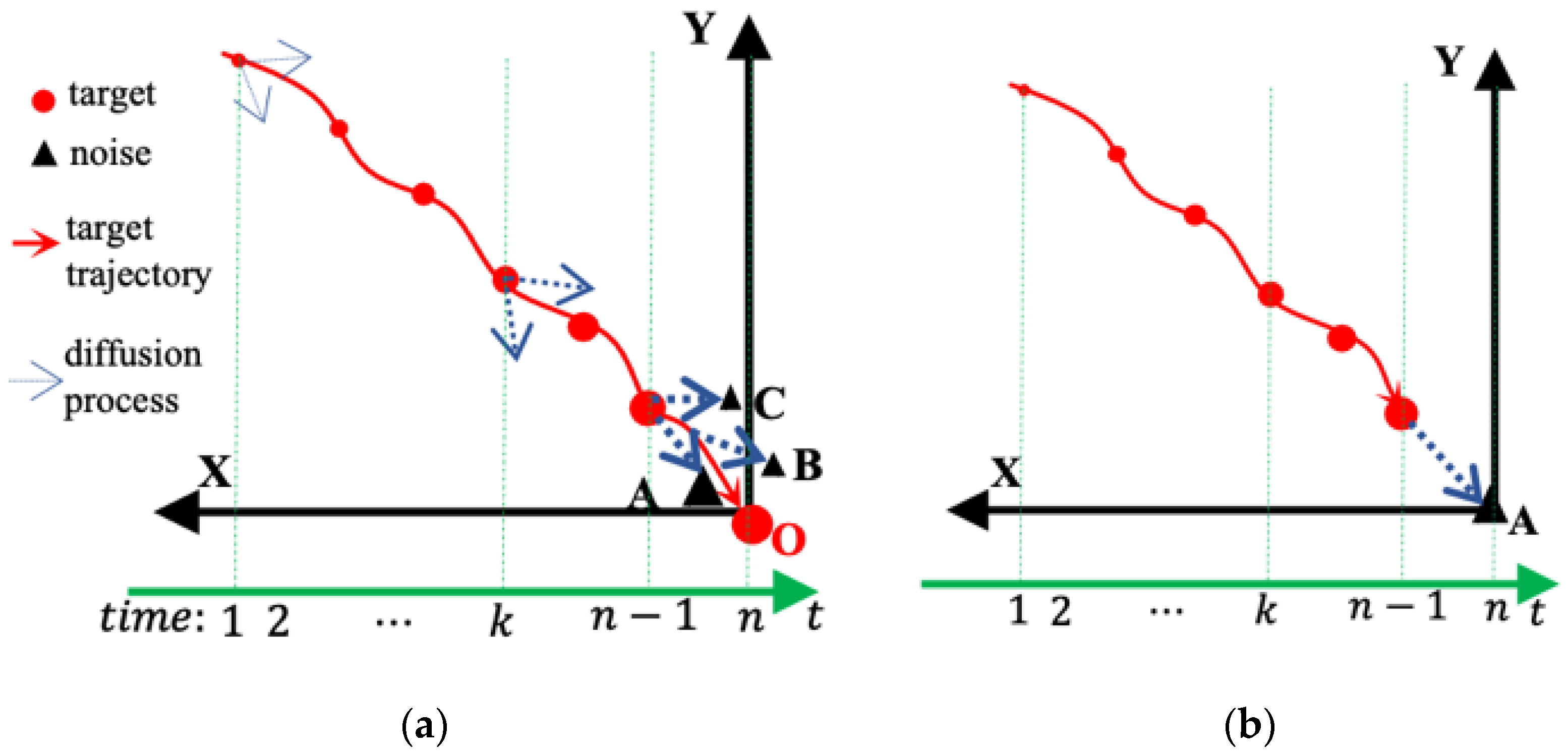
As in Figure 2a, the target position in the current frame is O x o , y o , and the target trajectory is the red curve in the XOY area with O as the origin point. When O is the point to be detected, energy accumulation based on the DP method is carried out in the X O Y area. The energy accumulation and diffusion process of the target is shown in Figure 2a, where the red dot indicates the result of energy accumulation along the target track during the accumulation process, and the blue arrow indicates the diffusion of the target energy. The larger the dot is, the greater the energy accumulated. The wider the arrow is, the more energy diffused, and the black triangular points A, B and C indicate the noise points with strong energy in the current frame. When the number of accumulated frames is very small (as in Figure 2a, t = 1 ), the accumulated target energy and the diffused energy are very small, which can be ignored. With a gradual increase in the accumulated frames (as t > k ), the accumulated target energy and the diffused energy increase gradually, which cannot be ignored. After the accumulation of previous n 1 frames, the accumulated energy of the target is E ( t = n 1 ) . From t = n 1 to t = n , the previous accumulated energy diffuses to the target point O (with energy E O ( t = n ) ) and the nearby noise point set A ,   B , C N (with energy E N ( t = n ) ) . At t = n , the energy of the target and the neighborhood noise is:
E t a r g e t = E t = n 1 + E O t = n E n o i s e = E t = n 1 + E A ,   B , C N t = n
According to (8), after energy accumulation, the probability that the energy of the target point is greater than that of the nearby noise point ( P r { E t a r g e t > E n o i s e } ) depends on the energy of the target and its nearby points in the current frame. When the target SCR is large (SCR > 3), P r { ( E t a r g e t > E n o i s e } is large because P r { E O ( t = n ) > E A ,   B , C N t = n } . However, with a decrease in the SCR, P r ( E t a r g e t > E n o i s e decreases because P r ( E O ( t = n ) > E A , B , C N t = n ) decrease, meaning that an increasing number of noise points are enhanced and more false alarms are generated.
2.
Quantitative Analysis
The analysis focuses on a popular DP method in which the maximum function m a x is the optimization process and the gray value is the stage merit function. Suppose that before processing, the noise obeys a Gaussian distribution N ~ μ , σ , the noise point energy is μ , the target point energy is T , and the number of accumulated frames is n .
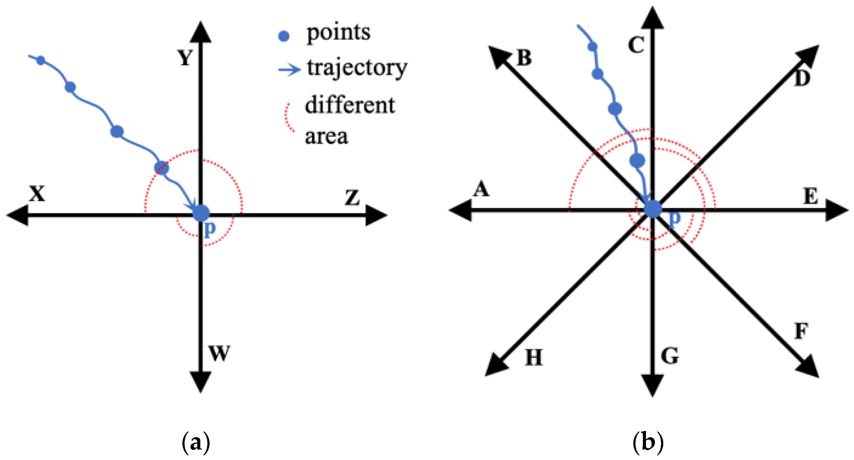
For each pixel P in the current image, as in Figure 3a, 4 accumulated energy values I x p y P , I y p z P , I z p w P , and I w p x P can be obtained after performing the DP method in 4 different areas {XPY, YPZ, ZPW, WPX}. There are three types of pixels in an image (see (9)): pixel P belongs to the target, noise is far from the target ( n o i s e _ f a r ), and noise is near the target ( n o i s e _ n e a r ).
P   t a r g e t ,   n o i s e _ n e a r ,   n o i s e _ f a r
Assume that when pixel P is the target, as in Figure 3a, the target trajectory C belongs to the X P Y area. After energy accumulation, the final energy of P is:
I P = m a x { I x p y P ,   I y p z P ,   I z p w P ,   I w p x P } = I x p y P = n T , P t a r g e t ,   C X P Y ; I x p y P = k T + n k μ ,   P n o i s e _ n e a r ,   C X P Y ; n μ ,   P n o i s e _ f a r , C 4   a r e a s   w i t h   equal   probability .
When pixel P belongs to noise that is near the target, in the trajectory of this kind of point, the first k points belong to the targets, while the last n k points belong to the noise. After accumulation, if SCR > 3, according to the 3 σ rule of thumb, then the probability that the target energy is larger than the noise is more than 99%. That is, on the energy accumulation map, the mean value of the probability distribution of the target point is greater than that of the noise point. However, when SCR < 3, this relation might be incorrect. As in Figure 2b, for noise point A with strong energy ( μ > T ), k = n 1 , after accumulation ( k T + n k μ ) > n T , which means E n o i s e > E t a r g e t . The lower the SCR is, the more noise points are enhanced after energy accumulation.
Another conclusion can be drawn from (10): If P t t a r g e t , then the corresponding trajectory C t of P t contains n target points; if P n e a r n o i s e _ n e a r , then the corresponding trajectory C n e a r of P n e a r contains k target points and n k noise points; if P f a r n o i s e _ f a r , then the corresponding trajectory C f a r of P f a r contains n noise points. After accumulation, whether the energy of P t is larger than that of P n e a r , the trajectories C t and C n e a r are in the same area. As shown in Figure 2, the trajectories of target point O and noise point A belong to areas XOY and XAY, respectively. Because the categories of points O and A are not known in advance, O and A are treated as one point P in the current image; thus, XOY and XAY are X P Y . Therefore, as long as the energy of C t or C n e a r is larger than that of trajectory C f a r , the target search area can be found via the following backtracking method:
m a x I m a p P m a x t a r g e t n o i s e _ n e a r C X P Y X P Y X P Y
First, for the accumulation map I m a p , the point with the largest energy P m a x can be found through the maximum function m a x . When the SCR is not very low, the following premise (12) is true. As above, the point P m a x belongs to t a r g e t or the target’s nearby noise ( n o i s e _ n e a r ) .
n T   o r   k T + n k μ >   n μ
Then, through P m a x and (10), find the area where the corresponding trajectory C m a x belongs and take the area as the target search area for each pixel.
Summarizing the above analysis, when using the DP method for energy accumulation under low SCR conditions, (1) the energy of the target will diffuse to the noise points and produce many false alarms; (2) if there is only one target, then the area to which the target trajectory belongs can be found according to the point with the largest energy (as the process in (11)), but this point cannot be taken as the target because it probably belongs to the noise.

2.1.3. Second Power Optimal Merit Function

As in the above analysis, the lower the SCR is, the more similar the probability distribution of the target and noise, and the smaller the probability of n T > n μ is, the larger the probability that the point with the largest energy P m a x belongs to the noise far from the target ( n o i s e _ f a r ). According to (10), when P m a x n o i s e _ f a r , it is impossible to find where the trajectory belongs because it belongs to 4 areas with equal probability. This means that the accuracy of finding the target trajectory according to (11) decreases under low SCR conditions.
Therefore, to solve the above problems, the second power optimal merit function-based DP method is proposed. It consists of four steps.
(1) As in Figure 3b, for each pixel P , 8 different search areas are set: A P C , B P D , C P E , D P F , E P G , F P H , G P A , H P B , the range of each area is 90°, all range is 360°, and the overlap angle between each two areas is 45°.
(2) In 8 search areas, for each pixel P , the DP method is performed, in which m a x is the optimization process and the gray value is the stage merit function to obtain 8 accumulated energy values I P .
I P = { I A P C ,   I B P D ,   I C P E ,   I D P F ,   I E P G ,   I F P H ,   I G P A ,   I H P B }
(3) For each pixel P , the optimal value is calculated according to the second power optimal merit function (14). Assume that when pixel P is the target, as in Figure 3b, target trajectory C belongs to A P C   and   B P D .
I o p t P = m a x { I 1 ,   I 2 ,   I 3 ,   I 4 ,   I 5 ,   I 6 ,   I 7 ,   I 8 } = m a x { I A P C × I B P D ,   I B P D × I C P E ,   I C P E × I D P F ,   I D P F × I E P G ,   I E P G × I F P H ,   I F P H × I G P A ,   I G P A × I H P B ,   I H P B × I A P C } = I 1 n T 2 , P t a r g e t ,   C A P C , B P D ; I 1 k T + n k μ 2 ,   P n o i s e _ n e a r ,   C A P C , B P D ; n μ 2 ,   P n o i s e _ f a r , C 8   a r e a s   w i t h   equal   probability .
(4) As in (11), the target search area is found via the following backtracking method.
m a x I m a p P m a x I i i 1 , 2 8 i a r e a   p a i r
where the a r e a   p a i r denotes the areas with overlaps.
a r e a   p a i r = { 1 : A P C & B P D ,   2 : B P D & C P E ,   3 : C P E & D P F ,   4 : D P F & E P G 5 : E P G & F P H ,   6 : F P H & G P A ,   7 : G P A & H P B ,   8 : H P B & A P C }
where A P C   &   B P D denotes the areas A P C and B P D .
The proposed second power optimal merit function essentially transforms the comparison of the target and noise trajectory energy from the first power (as in (12)) to the following second power.
n T 2   o r   k T + n k μ 2 > n μ 2
As long as premise (17) is true, this method can be used to find the area to which the target trajectory belongs.
According to the property of the power function:
y = x α
If x > 1 , with increasing α ( α > 0 ), y increases; if x > 1 and α > 1 , with increasing x , the slope of the curve and the derivative increase, meaning that a small increase in x will lead to a large increase in y .
According to the principle of ballistic trajectory integral (3), after accumulation, the probability ( P r ) that the target energy is greater than the noise energy is larger than the probability that the noise energy is greater than the target energy:
P r { E t a r g e t > E n o i s e } > P r { E n o i s e > E t a r g e t }
This means
P r { n T > n μ } > P r { n μ > n T }
When the accumulation frame number n > 1 , n T , n μ > 1 , from n T , n μ to n T 2 , n μ 2 , the increase in n T is larger than n μ , meaning there is a larger increase for the y of n T , according to the property of the power function and (20), the following relation can be deduced:
P r { n T 2 > n μ 2 } > P r { n T > n μ }
Similarly, for n T and k T + n k μ :
P r { k T + n k μ 2 > n μ 2 } > P r { k T + n k μ > n μ }
To find the area to which the target trajectory belongs, premises (12) and (17) must be true. Based on (21) and (22), it can be concluded that the probability of premise (17) being true is larger than that of premise (12), meaning the second power optimal merit function-based method is more reliable than the first power, in theory.
Similar to (11), the point with the largest energy P m a x in (15) can only be used to find the target search area but cannot be taken as the target because it probably belongs to the noise.
As in Figure 3b, point P is the target, and the target trajectory is the blue curve in the A P C area with P as the origin point. According to the proposed second power merit function-based DP ((12)–(15)), the area pair { A P C & B P D } can be obtained. Both A P C and B P D can be used as the target search area because both areas contain the target trajectory.
To accurately locate the position of the target, for each pixel to be detected, the next task is to find the possible trajectories in the target search area. Compared with an exhaustive search, this approach reduces the trajectory hypothesis space by 3 4 for each pixel.

2.2. Two-Stage MHT Model

2.2.1. The Proposed Parallel MHT Model

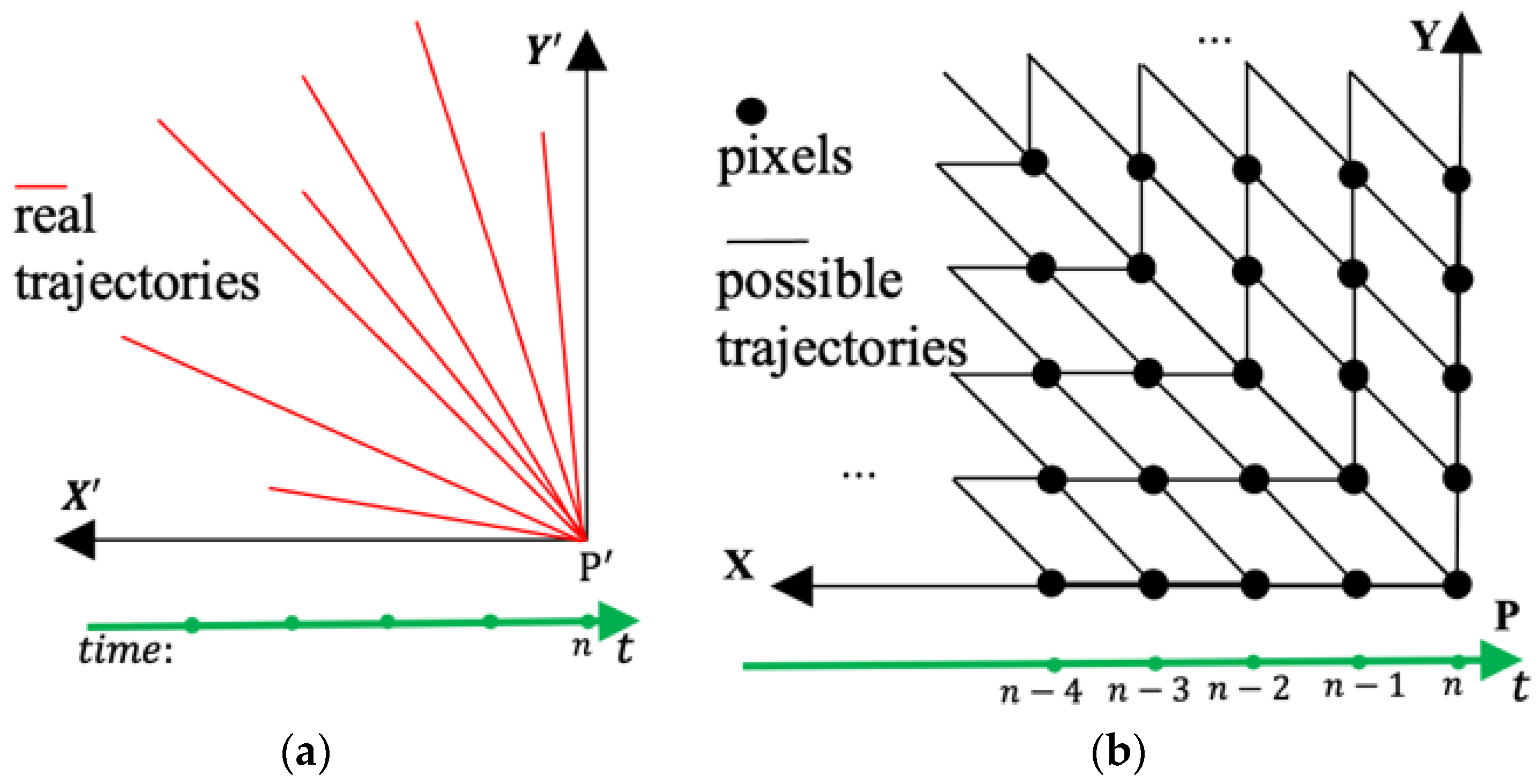
After the target search area is obtained, for each pixel in the current frame, the possible trajectories in the target search area need to be found. Since the sampling frequency of the infrared detector cannot completely match the moving speed of the target, if the target moves in a straight line in the real 2D space, then the imaging of the target is probably not a straight line in the discretized 2D image space. As in Figure 4a, in the 2D space the real trajectories that pass through point P are the red straight lines. If these lines are mapped to the 2D image space, then the trajectories are no longer straight lines but tree-structure-like curves that pass through point P , and the nodes of the curves are different pixels, as shown in Figure 4b. The number of trajectories m in the XPY area are related to the length of the sequence n .
m = 2 n 1
These trajectories have the following property. For the points in different positions on the current image, only the coordinates of nodes in each trajectory are different; the shape of the tree-structured trajectory space and the number of all trajectories are the same. This is called the ‘trajectory shape similarity property’ in this paper. To describe this property, the multiple trajectory hypotheses model Δ H t r e e is constructed. As in Figure 5, Δ H t r e e is a m × n 2-D matrix. The relative coordinates of all trajectories are saved in Δ H t r e e . As in Figure 5, Δ X n m denotes the relative coordinates Δ x , Δ y of the nth point in the mth trajectory. For the point at position P x , y , the tree-structured trajectory space can be described by H x , y .
H x , y = Δ H t r e e x , y
where denotes adding the coordinates of the current point x , y to each node in Δ H t r e e .For point P , after obtaining trajectories, the testing process is:
E P x , y = max 1 : m S 1 : n , M , N H x , y = max 1 : m I 1 , I 2 , I 3 , I m
where S denotes the infrared sequence with length n , the size of each frame is M × N , and 1 x M , 1 y N . denotes matching the node coordinates on each trajectory with the image gray value and accumulating energy for each trajectory. I m denotes the energy of the mth trajectory. max 1 : m denotes the testing process, which takes the trajectory with the largest energy as the trajectory for point P and the corresponding energy as the accumulated energy E P x , y . Equations (24) and (25) constitute the proposed MHT model. There are the following advantages:
(1) The trajectory search problem is simplified. Because of the ‘trajectory shape similarity property’, the tree-structured trajectory space for each point can be saved in H x , y using (24). In this way, a one-by-one search of root nodes in all trajectories is avoided, reducing the calculation cost and improving the efficiency of obtaining trajectory space. The larger the image resolution is, the larger reduction in calculations.
(2) The energy accumulation process can be implemented in parallel. The process of energy accumulation is independent of the trajectory order, so all trajectories can be operated in parallel. In actual operation, all trajectories can be allocated to different threads of different central processing units (CPUs). This means that (25) can be performed in different threads. This is very beneficial for improving the operability of the TBD method.
(3) Compared with the classical MHT method [13], the proposed MHT method considers both accuracy and efficiency. Under low SCR conditions, to ensure the detection probability, more nodes should be reserved in the early stage, and the redundant trajectories should be deleted in the later stage when the accumulated energy reaches a certain extent. The classical MHT is a multistage testing process, and some nodes will be deleted in each stage, causing the loss of accuracy. To avoid this loss, in the first stage of proposed MHT model, all trajectories and nodes are saved. In addition, the whole process of classical MHT includes the establishment of a tree-structured list and the judgment, insertion and deletion of the tree nodes. The computational complexity of the operation of the tree list is high. In the proposed MHT model, the operations involving the tree list are only (24). The only testing process is max 1 : m . The computational complexity is very low.

2.2.2. Two-Stage MHT Model

In the process of energy accumulation, the lower the target SCR is, the longer the length of the trajectory needed, and the larger the number of trajectories, meaning the larger the trajectory hypothesis space. As in (23), the number of trajectories m increases exponentially with increasing sequence length n . For example, from n = 15 to n = 30 , m changes from 3.3 × 10 4 to 1.1 × 10 9 . The trajectory length is only doubled, and the number of trajectories is increased by approximately 3.3 × 10 4 times, which brings much more computing and storage consumption than the benefits of energy accumulation. The main reason for this problem is the redundancy of the trajectory. As shown in Figure 6a, trajectory OP is one trajectory that accumulates from point O ( t = 1 ) to point P ( t = n ). For point P, when t = n + 1 , there are 3 possible trajectories: OPQ, OPR and OPS. OP is the overlapping trajectory. If OP is the target trajectory and n is relatively large, the energy of the target has been accumulated to a certain extent at point P. The OPQ, OPR and OPS contain the target trajectory OP, so the energy accumulated along the three trajectories may be similar. At this time, OPQ, OPR and OPS are redundant trajectories, and two of them should be removed. When n is small, the energy of the target has not been fully accumulated when reaching point P. In this case, any trajectory cannot be eliminated to ensure that the target trajectory is retained. Therefore, the premise of eliminating redundant trajectories is that the target energy has accumulated to a certain extent.
The two-stage search-based energy accumulation method can be used to reduce redundant trajectories, as shown in Figure 6b. In the first stage, from t = 1 to t = k , O is taken as the starting point, and energy is accumulated along the sparse trajectories. After accumulation, some trajectories are missed because the trajectories are sparse. In the second stage, starting from the missing point in the first stage, the energy is accumulated from t = k to t = n . After a two-stage search, not only is the number of redundant trajectories reduced but also the search of multiple trajectories is realized.
Therefore, to mitigate the contradiction between the redundant trajectories and the requirements of more trajectories under low SCR, the two-stage MHT model is proposed. For each point P x , y in the current frame, the two-stage MHT model is used to obtain the accumulated energy. It consists of three steps.
(1) In the first stage, from t = 1 to t = k , in the target search area XPY, as in (24) and (25), the proposed MHT model is used to obtain the tree-structured trajectory space and the accumulated energy E 1 P x , y .
E 1 P x , y = max 1 : k S 1 : k , M , N H x , y
(2) In the second stage, from t = k to t = n , in the opposite area X P Y , as in Figure 6c, the proposed MHT model is used to obtain E 2 P x , y .
E 2 P x , y = max k : n S n : k , M , N H x , y
In H x , y , the relative coordinates of all trajectories in X P Y are saved.
(3) For each point P, the final accumulated energy E P x , y is:
E P x , y = E 1 P x , y + E 2 P x , y
If k = n ÷ 2 , the trajectory number m 2 in the proposed two-stage MHT model is
m 2 = 2 × ( 2 0.5 × n 1 )
The ratio of m and m 2 is α :
α = m m 2 = 2 n 1 2 × ( 2 0.5 × n 1 ) 2 n 2 0.5 × n + 1 = 2 0.5 × n 1
α shows that with increasing trajectory length, compared with the proposed single-stage MHT, the trajectory hypothesis space of the two-stage MHT decreases exponentially. For example, when n = 30 , the trajectory number in the single-stage MHT is approximately 1.07 × 10 9 . Therefore, many trajectories make the trajectory space very difficult to store and calculate, and there is basically no operability. However, the trajectory number in the two-stage MHT is approximately 6.5 × 10 4 , making 30-frame-based energy accumulation possible.

2.3. Target Tracking Method

For each pixel of the current frame, after energy accumulation via two-stage MHT, the energy accumulation map can be obtained, and the candidate target points can be obtained by constant false alarm (CFAR) segmentation of the map.
To further eliminate false alarms, a target tracking method is designed. It consists two steps.
(1) All the reserved candidate points in the target search area are tracked.
(2) The discontinuous trajectories and the associated points are deleted.

2.4. Detection Framework

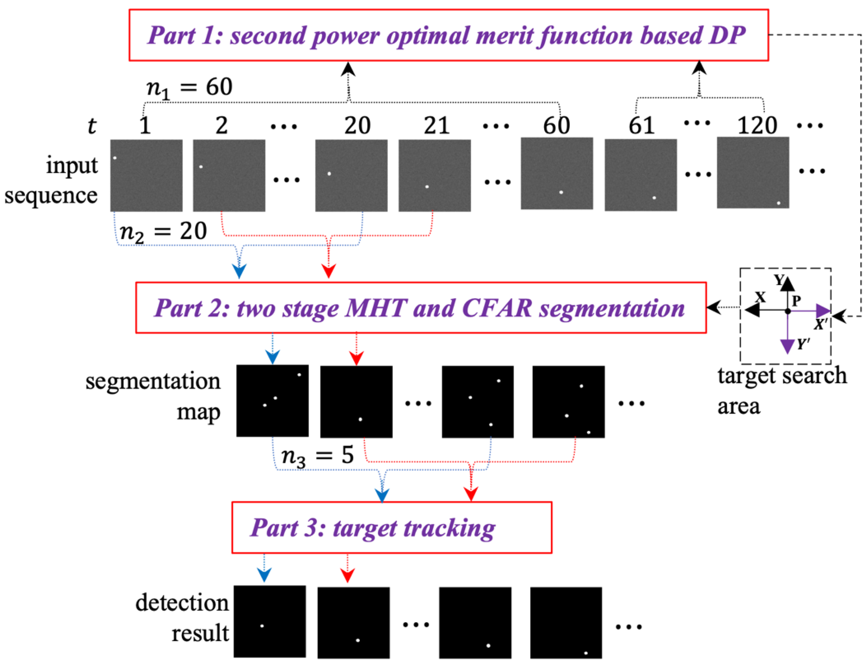
The DP–MHT–TBD detection framework is shown in Figure 7. It is a sequential detection process.
Part 1: Second power optimal merit function-based DP
The continuous n 1 frames are fed into the proposed second power optimal merit function-based DP to obtain the target search area XPY and its opposite area X P Y . These two areas are used in the next part. The flow of this part consists of four steps (the details can be seen from Formula (13) to (16) in Section 2.1.3).
Part 2: Two-stage MHT and CFAR segmentation
(1) The previous n 2 frames are used for energy accumulation. For each pixel P in the current frame, the proposed two-stage MHT model is used to accumulate energy along the trajectories only in areas XPY and X P Y . Once all the points have been processed, the energy accumulation map can be obtained. The flow of this part consists of three steps (the details can be seen from Formula (26) to (28) in Section 2.2.2).
(2) The CFAR segmentation method is used to segment the energy accumulation map to obtain the candidate points of the current frame. In the segmentation process, the threshold T h is set according the pre-set false alarm rate F a .
T h = l n F a
Part 3: Target tracking
All the reserved candidate points are tracked, the discontinuous trajectories are found, and the candidate points in the discontinuous trajectories to noise are classified. The flow of this part consists of two steps (the details can be seen in Section 2.3).
3. Experiments and Analysis

To verify the proposed algorithm, experiments regarding the proposed second power optimal merit function-based DP, two-stage MHT and target tracking were carried out.

3.1. Datasets and Evaluation Setup

In practical applications, it is difficult to obtain the IR data of space point targets, so an IR image with low SCR is simulated first. Some images are shown in Figure 1b. When building the simulation image, the noise function of MATLAB is first used to add Gaussian noise ( N ~ μ , σ ) to a blank 256 × 256 image to obtain the background B . The mean value μ and the standard deviation σ of the background are 90 and 10, respectively. Then, according to an SCR value, as in (32), the target T is only set at one certain position in each image. In the datasets, the target occupies only one pixel in each frame and the target motion speed is 1 pixel per frame.
T = B + S C R × σ
The targets in the infrared sequence simulated according to the above process obey normal distribution, making the simulated datasets more reasonable and more correspondent with the actual infrared point target scene.
The target search area detection probability P a r e a is used to verify whether the proposed second power DP can correctly find the target search area.
P a r e a = n u m b e r   o f   c o r r e c t   d e t e c t i o n s n u m b e r   o f   e x p e r i m e n t s
The detection probability P d and the false alarm rate F a are used as the evaluation metrics for target detection, and P d and F a are the ordinate and the abscissa of the receiver operating characteristic (ROC) curve, respectively [4].
P d = n u m b e r   o f   t r u e   d e t e c t i o n s n u m b e r   o f   actual   targets
F a = n u m b e r   o f   f a l s e   d e t e c t i o n s n u m b e r   o f   i m a g e s
The detected target is considered true if it simultaneously meets two requirements: (1) the center of the ground truth is detected and (2) the pixel distance between the center of the ground truth and the result is less than 2 pixels (Manhattan distance).
All the experiments were implemented with MATLAB R2019 and C++ in Ubuntu 16.04 on a PC with a 4-core CPU and 16-GB RAM.

3.2. Experiments on Second Power Optimal Merit Function-Based DP

A total of 1000 sets of sequences with different lengths and different SCRs are used to verify the proposed second power optimal merit function-based DP.

3.2.1. The Second Power Optimal Merit Function-Based DP

To determine the advantage and validity of the proposed method, a comparative experiment with respect to the first/second power optimal merit function-based DP is carried out. The SCR of the sequences used in the experiment is 1.5. The comparison results are shown in Table 1, where n denotes the number of frames used in different methods.
From the comparison result (see Table 1), the following conclusions can be drawn:
(1) In a very low SCR condition (SCR = 1.5), no matter how many frames are used, and whether the first or second power function-based DP is used, P a r e a > P d . For example, when using 60 frames of images, the target search area detection probability is 98.57%, while the target detection probability is only 78.76%. As in Table 1, the P d value of all methods is less than 80%. These data show that using the DP method to find the target search area is more reliable than directly detecting the target position.
(2) P a r e a increases with the number of frames used in the energy accumulation. However, this parameter does not grow linearly but grows more slowly. For example, when n increases from 45 to 60, P a r e a increases approximately 3.3%. However, when n increases from 60 to 75, P a r e a only increases approximately 0.1%. P d increases with the number of frames, but is not necessarily larger as the number of frames continues to increase. For example, compared with n = 60 , when n = 75 , P d decreases by approximately 5%.
(3) The first power DP and the second power DP accumulate energy in four and eight areas, respectively, so the time cost of the second power DP is twice that of the first power DP. However, even if 60 frames are used, it only takes 1.6 s to find the target search area. In practical applications, the more frames that are used, the greater the amount of calculation and the worse the real-time performance. After comprehensive consideration of various factors, the appropriate n is 60.

3.2.2. The SCR of the Infrared Sequence

In each different SCR (from 1 to 1.5), 1000 sets of sequences are used to investigate the performance of the proposed method. The length n of every sequence is 60.
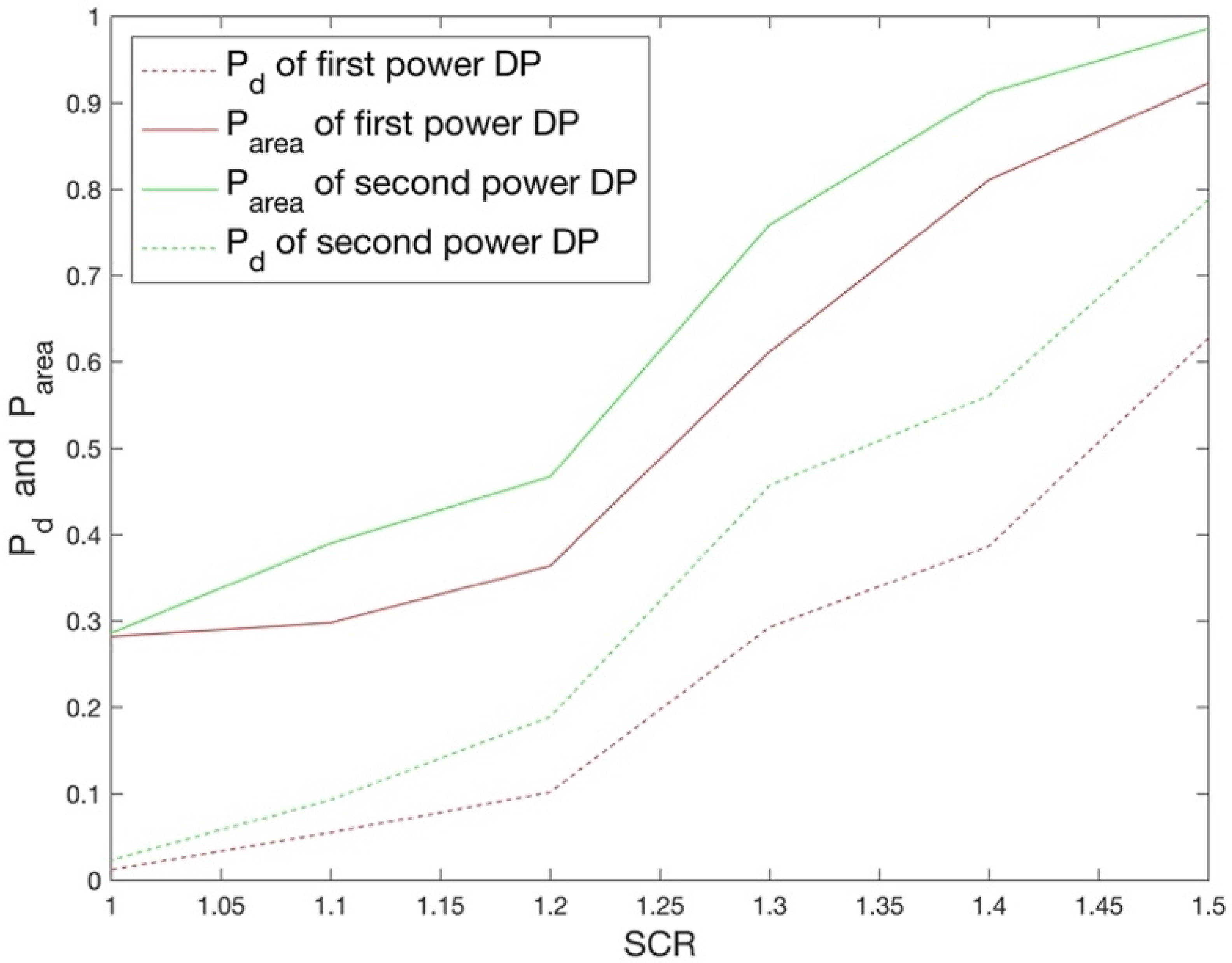
The P a r e a and P d performances are shown in Table 2 and Figure 8. The following conclusions can be drawn from the results:
(1) In different SCRs, the performance of the proposed second power DP is better than that of the original first power DP. As shown in Figure 8, the P a r e a and P d curves of the second power DP are always above the curve of the first power DP, showing the advantages of the second power DP. In addition, the P a r e a curves of different methods are above the PD curves, further showing that using the DP method to find the target search area is more reliable than directly detecting the target position.
(2) As the SCR decreases, P a r e a decreases rapidly. For the proposed second power DP, when S C R 1.3 , P a r e a is less than 80%, and when S C R 1.2 , P a r e a is less than 50%, indicating that the effect of the proposed method is not good when the S C R < 1.4 . The subsequent target detection part is based on the correct detection of the target search area. If P a r e a is less than 90%, even if the P d of the subsequent MHT part is very high, then the final detection probability will not be very high.

3.3. Experiments on Two-Stage MHT

The condition of the proposed MHT is that the target search area is correctly determined by the proposed DP. Event A is defined as the target search area correctly found by the proposed DP, while event B is defined as the target correctly detected by the proposed MHT. The target detection probability of the DP–MHT–TBD is P d p m h t t b d . In this work, P a r e a = P A and P d p m h t t b d = P A B According to the conditional probability formula, P A B is:
P A B = P A × P ( B | A )
where P ( B | A ) denotes the conditional probability. Therefore, to obtain P ( B | A ) , experiments were carried out on the basis of event A being true.
According to above analysis, when S C R 1.4 , the proposed DP can find the target search area with probability greater than 90. The MHT-based target detection part is based on the target search area. Therefore, this section only investigates the performance of the proposed two-stage MHT when SCR 1.4 . A total of 1000 sets of sequences with different lengths n are used to verify the performance of the proposed MHT, and the target SCR of each sequence is 1.5 or 1.4. The ROC curves are shown in Figure 9, and the P d and time cost are shown in Table 3 and Table 4, respectively. In this section, P d = P ( B | A ) .
From the results, the following conclusions can be drawn:
(1) The more images used, the better the performance but the greater the amount of calculation. As shown in Figure 9, the larger n is, the closer the ROC curve is to the top left corner, indicating that the more images used, the greater the energy accumulated in the energy accumulation process, the higher the target detection probability and the lower the false alarm rate. With increasing n , the amount of calculation also increases. For example, when n = 30 , the time cost is 33 s, which means that it takes approximately 9 h to perform 1000 experiments. The amount of calculation is too large, so n is less than 28 in the experiment.
(2) The performance decreases with decreasing SCR. As in Table 3 and Table 4, to meet the dual requirements of F a < 0.1 % and P d > 90 % , when SCR is 1.5 and 1.4, the minimum number of images required is approximately 16 and 20, respectively.
After obtaining P A and P ( B | A ) , according (36), the final target detection probability of the DP–MHT–TBD P d p m h t t b d can be obtained. When F a = 0.1 % , P d p m h t t b d is shown in Table 5. When SCR is 1.5, the proposed DP–MHT–TBD can detect the target in the image sequence with a detection probability of more than 90%.

3.4. Experiments on Target Tracking

After CFAR segmentation of the energy accumulation map, candidate points can be obtained. However, the candidate points contain both targets and noise.
The energy accumulation maps are obtained by the two-stage MHT in which 20 frames are used for energy accumulation. Then, the CFAR segmentation method is used to segment 450 continuous energy accumulation maps. In the target tracking part, the trajectories that are discontinuous in five continuous segmentation maps are deleted, and the associated points are classified as noise. For each operation, the time cost is 0.003 s. The change in F a before and after target tracking is shown in Table 6. It can be seen that the target tracking method can eliminate false alarms by an order of magnitude.

3.5. Comparison Experiments

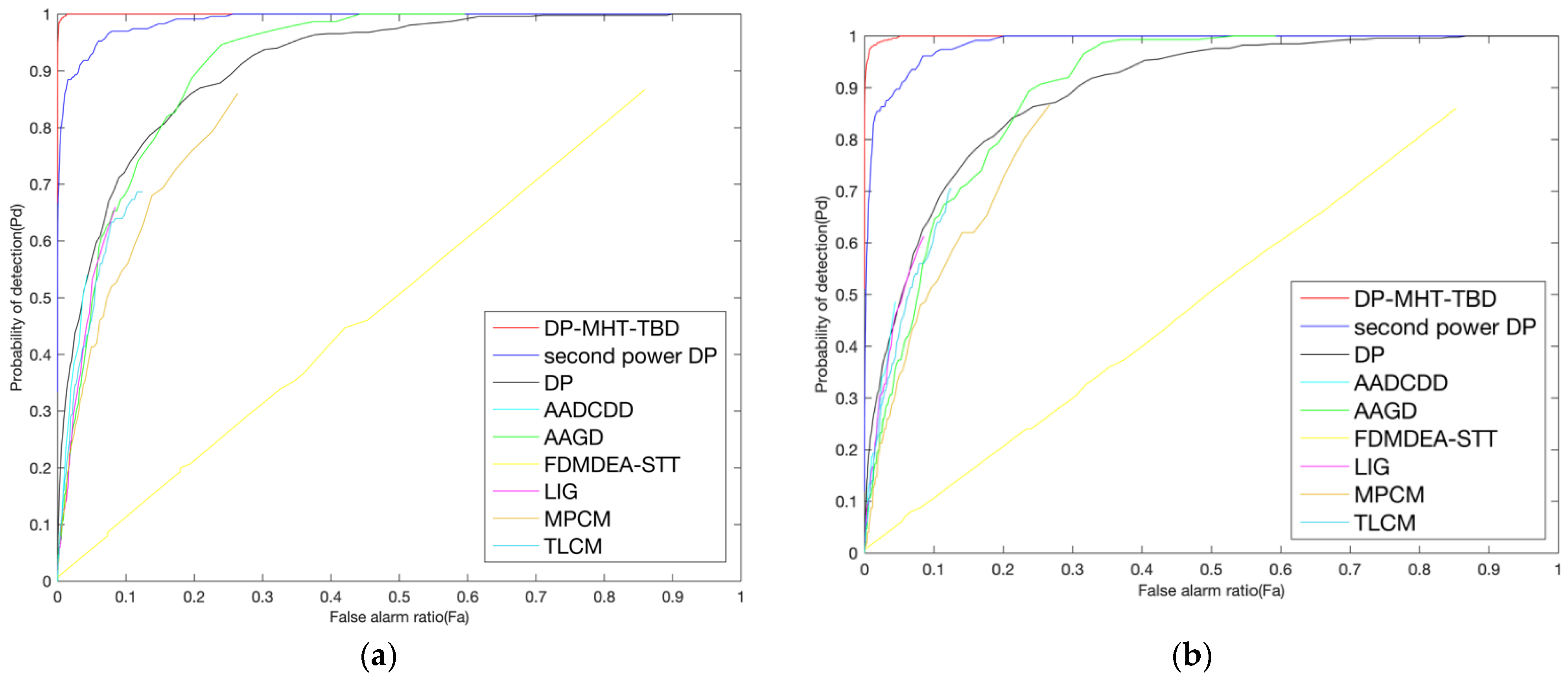
To verify the superiority of the proposed DP–MHT–TBD, three kinds of methods should be compared: TBD, DBT and DL Methods. However, this work focuses on the detection of the 1 × 1 point target under low SCR condition (SCR = 1.5). There is no shape and texture information in the 1 × 1 point target. It is difficult to train the neural networks with a sample in which there is only grey information of one pixel. Many deep learning methods were tested in the experiment, such as Faster-RCNN, the previous work’s spatial–temporal based method [1], TSDF [2] and so on. In these methods, the neural network could not learn the useful features and the network could not achieve coverage during the training process. To the best of our knowledge, there is no deep learning method that could detect the infrared point target under low SCR (SCR = 1.5). Thus, there are no experiments about deep learning methods in this work. In addition, the point target detection task under low SCR is usually related to the military field; it is difficult to obtain relevant code due to confidentiality rules or technical reasons. Considering the above factors, the following representative DBT and TBD methods are selected: DBT: LIG [6], multiscale patch-based contrast measure (MPCM) [28], absolute average gray difference (AAGD) [29], absolute average difference weighted by cumulative directional derivatives (AADCDD) [30] and LCM utilizing a tri-layer (TLCM) [31]; TBD: DP [12], second power optimal merit function-based DP, and facet derivative-based multidirectional edge awareness with spatial–temporal tensor (FDMDEA-STT) [32]. The experimental parameters and time cost of all methods are listed in Table 7. The ROC curves are shown in Figure 10. Some CFAR segmentation maps are shown in Figure 11.
From the results, it can be seen that:
(1) The proposed DP–MHT–TBD is superior to other methods with respect to the detection probability and false alarm rate. The proposed second power DP has better performance than the original DP.
(2) The proper energy accumulation method is the key to the detection of dim point targets. Only the proposed DP–MHT–TBD can detect the target because the energy of the point target is accumulated through the right way. In other methods, the target energy is not accumulated (in single-frame detection methods and FDMDEA-STT), or there is a serious diffusion of energy during the accumulation process (in DP and second power DP); the target is missed after segmentation because the energy of the target point is not superior to that of the noise point.
(3) The consumption time of the DP–MHT–TBD is greater than that of the other methods because there are more images to be processed. The proposed method is a sequential detection process and the image processing speed can be accelerated by using GPU or other ways, having high practical application values.
In brief, in Section 3, experiments on the proposed second power optimal merit function-based DP, two-stage MHT, target tracking and comparison methods are carried out. The results of each part verify the superiority of the corresponding part. When SCR is 1.5, 60 images (image size is 256 × 256 ) are used in the second power optimal merit function-based DP to find the target search area, 20 images are used in the two-stage MHT to accumulate energy, and 5 segmentation maps are used in target tracking to further eliminate false alarms. According to Table 2, Table 5 and Table 6, the proposed DP–MHT–TBD can detect a single point target in the image sequence with a detection probability above 90% and a false alarm rate of below 0.01%.

4. Discussion

Several observations from experimental and quantitative analysis are discussed.
First, theoretical and experimental studies have shown that the proposed second power optimal merit function-based DP outperforms the original DP. The proposed second power DP is used to find the target search area instead of directly detecting the target, avoiding the influence of agglomeration effect and reducing the trajectory hypothesis space.
Second, the proposed two stage parallel MHT is the key to detecting a point target under low SCR. This can be attributed to the fact that the novel parallel MHT structure and the two-stage strategy simplifies the trajectory search problem and reduces the hypothesis space exponentially. This enables the energy accumulation process of dim targets to be very efficient.
Third, as the SCR decreases, the point detection task becomes more and more difficult. The gain is finite by only using infrared data or improving TBD methods. Some potential ideas should be considered. (1) The idea of adaptive spatial–temporal context [33] can be used to improve the robustness of the tracking part in the TBD. (2)The multi-sensor data fusion [34,35] may be a valuable project for theoretical investigation and practical application in the dim point detection field. With the development of detector technology, it will be easy to obtain radar, infrared, hyperspectral and other data. If these data can be fused to take advantage of their respective advantages, it will be of great help in reducing the trajectory hypothesis space, improving processing efficiency and detection capability.

5. Conclusions

In this paper, a novel and accurate DP–MHT–TBD (dynamic programming–multiple hypothesis testing–track before detect) algorithm is proposed for infrared dim point target detection. The method consists of three parts: the second power optimal merit function-based DP, two-stage MHT and target tracking. In particular, first, for each point to be detected, the second power optimal merit function-based DP is used to find the target search area to reduce the trajectory hypothesis space. Next, the two-stage MHT, which can further reduce the trajectory hypothesis space exponentially and mitigate the contradiction between the redundant trajectories and the requirements of more trajectories under low SCR (signal-to-clutter ratio), is used to save the tree-structured trajectory space and accumulate energy in parallel. Finally, after CFAR (constant false alarm) segmentation of the accumulation map, the target tracking method is used to further eliminate false alarms. Via experiments on each part and comparison methods, the proposed DP–MHT–TBD algorithm, which takes advantage of the small computation cost of DP and high accuracy of exhaustive search, greatly reduces the computational cost and storage requirements, showing superior ability in detecting point targets under low SCR conditions. The point target detection task under low SCR is difficult but significant. Although the proposed method has engineering applicability and good detection performance, it can only detect a single point target. In future work, the studies could be conducted from the following aspects: the combination of TBD and deep learning methods, the use of adaptive spatial–temporal context information and the fusion of multi-sensor data.

Author Contributions

Conceptualization, J.D. and H.L.; methodology, J.D. and H.L.; software, J.D. and Y.D.; validation, J.D., L.Z. and M.H.; formal analysis, L.Z. and M.H.; investigation, X.S. and D.L.; resources, J.D. and Y.Z.; writing—original draft preparation, J.D.; writing—review and editing, J.D. and H.L.; visualization, D.L., Y.D. and Y.Z.; project administration, X.S. All authors have read and agreed to the published version of the manuscript.

Funding

This work was supported by the National Natural Science Foundation of China (61901489).

Data Availability Statement

Not applicable.

Acknowledgments

The authors would like to thank the editors and the reviewers for their valuable suggestions.

Conflicts of Interest

The authors declare no conflict of interest.

References

  1. Du, J.M.; Lu, H.Z.; Zhang, L.P.; Hu, M.F.; Chen, S.; Deng, Y.J.; Shen, X.; Zhang, Y. A Spatial-Temporal Feature-Based Detection Framework for Infrared Dim Small Target. IEEE Trans. Geosci. Remote Sens. 2022, 60, 1–12. [Google Scholar] [CrossRef]
  2. Du, J.M.; Lu, H.Z.; Hu, M.F.; Zhang, L.P.; Shen, X.L. CNN-based infrared dim small target detection algorithm using target-oriented shallow-deep features and effective small anchor. IET Image Process. 2021, 15, 1–15. [Google Scholar] [CrossRef]
  3. Ren, X.; Wang, J.; Ma, T.; Zhu, X.; Bai, K.; Wang, J. Review on Infrared Dim and Small Target Detection Technology. J. Zhengzhou Univ. 2020, 52, 1–21. [Google Scholar] [CrossRef]
  4. Zhang, P.; Zhang, L.; Wang, X.; Shen, F.; Pu, T.; Fei, C. Edge and Corner Awareness-Based Spatial–Temporal Tensor Model for Infrared Small-Target Detection. IEEE Trans. Geosci. Remote Sens. 2021, 59, 10708–10724. [Google Scholar] [CrossRef]
  5. Chen, C.L.P.; Li, H.; Wei, Y.; Xia, T.; Tang, Y.Y. A Local Contrast Method for Small Infrared Target Detection. IEEE Trans. Geosci. Remote Sens. 2014, 52, 574–581. [Google Scholar] [CrossRef]
  6. Zhang, H.; Zhang, L.; Yuan, D.; Chen, H. Infrared small target detection based on local intensity and gradient properties. Infrared Phys. Technol. 2018, 89, 88–96. [Google Scholar] [CrossRef]
  7. Gao, C.; Meng, D.; Yang, Y.; Wang, Y.; Zhou, X.; Hauptmann, A.G. Infrared Patch-Image Model for Small Target Detection in a Single Image. IEEE Trans. Image Process. 2013, 22, 4996–5009. [Google Scholar] [CrossRef]
  8. Reed, I.S.; Gagliardi, R.M.; Shao, H.M. Application of Three-Dimensional Filtering to Moving Target Detection. IEEE Trans. Aerosp. Electron. Syst. 1983, 19, 898–905. [Google Scholar] [CrossRef]
  9. Carson, B.D.; Evens, E.D.; Wilson, S.L. Search radar detection and track with the Hough transform part I: System concept. IEEE Trans. Aerosp. Electron. Syst. 1994, 30, 102–108. [Google Scholar] [CrossRef]
  10. Carson, B.D.; Evens, E.D.; Wilson, S.L. Search radar detection and track with the Hough transform Part II: Detection statistics. IEEE Trans. Aerosp. Electron. Syst. 1994, 30, 109–115. [Google Scholar] [CrossRef]
  11. Carson, B.D.; Evens, E.D.; Wilson, S.L. Search radar detection and track with the Hough transform Part III: Detection performance with binary integration. IEEE Trans. Aerosp. Electron. Syst. 1994, 30, 116–125. [Google Scholar] [CrossRef]
  12. Barniv, Y. Dynamic Programming Solution for Detecting Dim Moving Targets. IEEE Trans. Aerosp. Electron. Syst. 1985, 21, 144–156. [Google Scholar] [CrossRef]
  13. Blostein, S.D.; Huang, T.S. Detecting small, moving objects in image sequences using sequential hypothesis testing. IEEE Trans. Signal Process. 1991, 39, 1611–1629. [Google Scholar] [CrossRef] [Green Version]
  14. Liu, W.; Anguelov, D.; Erhan, D.; Szegedy, C.; Reed, S.; Fu, C.Y.; Berg, C. SSD: Single shot multibox detector. In Proceedings of the 14th European Conference on Computer Vision (ECCV 2016), Amsterdam, The Netherlands, 8–16 October 2016. [Google Scholar] [CrossRef] [Green Version]
  15. Redmon, J.; Divvala, S.; Girshick, R.; Farhadi, A. You Only Look Once: Unified, Real-Time Object Detection. In Proceedings of the 2016 IEEE Conference on Computer Vision and Pattern Recognition (CVPR 2016), Las Vegas, NV, USA, 26–30 June 2016. [Google Scholar] [CrossRef] [Green Version]
  16. Ren, S.; He, K.; Girshick, R.; Sun, J. Faster R-CNN: Towards Real-Time Object Detection with Region Proposal Networks. IEEE Trans. Pattern Anal. Mach. Intell. 2017, 39, 1137–1149. [Google Scholar] [CrossRef] [PubMed] [Green Version]
  17. Zhao, M.; Li, C.; Xu, Y.; Peng, F.; Liu, L.; Wu, N. TBC-Net: A real-time detector for infrared small target detection using semantic constraint. arXiv 2019, arXiv:2001.05852. [Google Scholar] [CrossRef]
  18. Lin, H.U.; Wang, S.Y.; Wan, Y. Improvement on Track-Before-Detection Algorithm Based on Dynamic Programming. J. Air Force Radar Acad. 2010, 24, 79–82. [Google Scholar] [CrossRef]
  19. Gao, F.; Zhang, F.; Zhu, H.; Sun, j.; Wang, J. An improved TBD algorithm based on dynamic programming for dim SAR target detection. In Proceedings of the 12th International Conference on Signal Processing (ICSP 2014), Bangkok, Thailand, 19–21 November 2014. [Google Scholar] [CrossRef]
  20. Lyu, T.J.; Yuan, Z.Q.; Lei, G.; Ren, Z. A DP-TBD Algorithm under Complex Clutter Environment. Fire Control. Radar Technol. 2021, 50, 78–81. [Google Scholar] [CrossRef]
  21. Xing, H.; Suo, J.D.; Sun, B. Dynamic programming track⁃before⁃detect algorithm with improved state transition set. Mod. Electron. Tech. 2020, 43, 1–5. [Google Scholar] [CrossRef]
  22. Guo, Q.; Li, Z.; Song, W.; Fu, W. Parallel Computing Based Dynamic Programming Algorithm of Track-before-Detect. Symmetry 2018, 11, 29. [Google Scholar] [CrossRef] [Green Version]
  23. Wang, Y. The Study of Weak Target Track before Detect Algorithm Basing on Dynamic Programming. Master’s Thesis, Yanshan University, Qinhuangdao, China, 2017. [Google Scholar]
  24. Dong, J. Tracking before Detection Based on Dynamic Programming (DP-TBD) Algorithm. Master’s Thesis, Dalian Maritime University, Dalian, China, 2017. [Google Scholar]
  25. Chen, H.; Sun, G.F.; Lu, H.Z.; Chen, S.F. Detection Algorithm for Small Moving Targets Based on Dynamic Programming and Confidence Test. Syst. Eng. Electron. 2003, 25, 472–475. [Google Scholar] [CrossRef]
  26. Chen, S.F.; Xiao, S.Z.; Lu, H.Z. Dim targets detection based on multi-regions dynamic programming and track matching. Infrared Laser Eng. 2007, 36, 738–741. [Google Scholar] [CrossRef]
  27. Chen, S.F.; Xiao, S.Z.; Lu, H.Z. An algorithm of low SNR small targets real-time detection in imagery. Signal Process. 2009, 25, 601–606. [Google Scholar] [CrossRef]
  28. Wei, Y.T.; You, X.; Li, H. Multiscale patch-based contrast measure for small infrared target detection. Pattern Recognit. 2016, 58, 216–226. [Google Scholar] [CrossRef]
  29. Deng, H.; Sun, X.; Liu, M.; Ye, C.; Zhou, X. Infrared small-target detection using multiscale gray difference weighted image entropy. IEEE Trans. Aerosp. Electron. Syst. 2016, 52, 60–72. [Google Scholar] [CrossRef]
  30. Aghaziyarati, S.; Moradi, S.; Talebi, H. Small infrared target detection using absolute average difference weighted by cumulative directional derivatives. Infrared Phys. Technol. 2019, 101, 78–87. [Google Scholar] [CrossRef]
  31. Han, J.; Moradi, S.; Faramarzi, I.; Liu, C.; Zhang, H.; Zhao, Q. A Local Contrast Method for Infrared Small-Target Detection Utilizing a Tri-Layer Window. IEEE Geosci. Remote Sens. Lett. 2020, 17, 1822–1826. [Google Scholar] [CrossRef]
  32. Pang, D.; Shan, T.; Li, W.; Ma, P.; Tao, R.; Ma, Y. Facet Derivative-Based Multidirectional Edge Awareness and Spatial–Temporal Tensor Model for Infrared Small Target Detection. IEEE Geosci. Remote Sens. 2022, 60, 1–15. [Google Scholar] [CrossRef]
  33. Mehmood, K.; Jalil, A.; Ali, A.; Khan, B.; Murad, M.; Khan, W.U.; He, Y.G. Context-Aware and Occlusion Handling Mechanism for Online Visual Object Tracking. Electronics 2021, 10, 43. [Google Scholar] [CrossRef]
  34. Stateczny, A.; Kazimierski, W. Multisensor Tracking of Marine Targets-Decentralized Fusion of Kalman and Neural Filters ehmood. Int. J. Electron. Telecommun. 2011, 57, 65–70. [Google Scholar] [CrossRef]
  35. Liu, W.; Liu, Y.; Bucknall, R. Filtering based multi-sensor data fusion algorithm for a reliable unmanned surface vehicle navigation. J. Mar. Eng. Technol. 2022, 1–17, Early Access. [Google Scholar] [CrossRef]
Figure 1. Representative infrared images with various backgrounds. (a) Background clutter is spatially nonstationary but temporally stationary; (b) Background clutter is temporally nonstationary, the area in red frame is the target and its neighbor pixels.
Remotesensing 14 05072 g001
Figure 2. Target energy accumulation and diffusion in the DP process. (a) Energy accumulation and diffusion process of target; (b) Diffusion effect for noise.
Remotesensing 14 05072 g002
Figure 3. DP-TBD in different areas. For each pixel, (a) DP process in 4 areas; (b) DP process in 8 areas.
Remotesensing 14 05072 g003
Figure 4. Possible trajectories in the target search area: (a) the trajectories in 2D space and (b) the trajectories in 2D image space. It is a tree-structured trajectory space.
Remotesensing 14 05072 g004
Figure 5. Proposed multiple trajectory hypotheses model Δ H t r e e . Δ X n m denotes the relative coordinates Δ x , Δ y of the nth point in the mth trajectory.
Remotesensing 14 05072 g005
Figure 6. Redundant and sparse trajectories: (a) redundant trajectories; (b) sparse trajectories; and (c) target search area and its opposite area.
Remotesensing 14 05072 g006
Figure 7. Proposed DP–MHT–TBD detection framework. It consists of the second power optimal merit function-based DP, two stage MHT and CFAR segmentation, target tracking. It is a sequential detection process.
Remotesensing 14 05072 g007
Figure 8. P a r e a and P d of different method at different SCRs.
Remotesensing 14 05072 g008
Figure 9. ROC curves of two stage MHT. n denotes the number of used images. (a) ROC curves when SCR is 1.4; (b) ROC curves when SCR is 1.5.
Remotesensing 14 05072 g009
Figure 10. ROC curves of different methods under different data. (a) SCR is 1.5; (b) SCR is 1.4.
Remotesensing 14 05072 g010
Figure 11. Detection results of the different methods. (a) 3-D display of the input image; (b) 9 × 9 neighborhoods of the target; (c) input image, SCR is 1.5; (dg) are CFAR segmentation maps of different methods: (d) two stage MHT; (e) second power DP; (f) DP; (g) AAGD; (h) final result of DP–MHT–TBD. In the CFAR segmentation process, Fa = 0.01%.
Remotesensing 14 05072 g011
Table 1. Quantitative comparison of DP.
Methodsn P a r e a (%) P d (%) Time
first power DP3068.7644.760.4 s
second power DP3080.7661.620.8 s
first power DP4586.1056.380.6 s
second power DP4595.3373.051.2 s
first power DP6092.2962.760.8 s
second power DP6098.5778.761.6 s
first power DP7592.8457.001 s
second power DP7598.6974.342 s
Table 2. Performance of the proposed DP with different SCRs.
SCR:1.51.41.31.21.11
Methods
P a r e a of first power DP92.381.161.236.429.828.2
P d of first power DP62.838.729.310.25.51.2
P a r e a of second power DP98.691.275.946.739.028.6
P d of second power DP78.856.145.718.99.32.3
Table 3. P ( B | A ) when SCR is 1.4.
n81216202428
F a
0.197.6998.1898.7999.1399.6999.89
0.0177.2389.5794.6396.8897.6298.79
0.00141.3367.0183.7990.1095.7798.12
0.000119.3535.6658.7976.5486.0794.83
time0.01 s0.03 s0.15 s0.74 s3.5 s16 s
Table 4. P ( B | A ) when SCR is 1.5.
n81216202428
F a
0.197.7998.3999.7299.7299.98100
0.0181.4694.2997.5498.5899.1099.12
0.00152.4273.8089.9194.7697.6498.97
0.000128.4349.8072.0886.6593.4097.92
time0.01 s0.03 s0.15 s0.74 s3.5 s16 s
Table 5. P(dpmhttbd) with Fa = 0.001.
n81216202428
SCR
1.437.6961.1176.4282.1787.3489.49
1.551.6972.7788.6593.4396.2797.58
time0.01 s0.03 s0.15 s0.74 s3.5 s16 s
Table 6. Fa after target tracking.
F a 0.10.010.0010.0001
SCR
1.50.0330.00100.000070.0000062
1.40.0460.00150.00010.0000078
Table 7. Parameter setting and time cost of different methods.
MethodsParameter SettingTime Cost
AADCDD [30]local window size: N = 3 ,   5 ,   7 0.01 s
AAGD [29]internal and external window size N = 3 ,   5 ,   7 0.005 s
LIG [6]window size: N = 3 ; ratio κ = 0.2 0.6 s
MPCM [28]cell size: N = 3 ,   5 ,   7 0.04 s
TLCM [31]window size: N = 3 ,   5 ,   7 0.56 s
FDMDEA-STT [32] λ = 0.1 ,   t = 3 ,   ρ = 1.05 , ϵ = 10 7 1.5 s
DP [12]20 frames are used to accumulate energy0.07 s
second power DP20 frames are used to accumulate energy0.07 s
Proposed60 frames are used to find the target search area
20 frames are used to accumulate energy
5 segmentation maps are used to eliminate false alarms
1.6 s
0.74 s
0.003 s
Publisher’s Note: MDPI stays neutral with regard to jurisdictional claims in published maps and institutional affiliations.