Article

Comparison between Different TomoSAR Imaging Models for Airborne Platform Flying at Low Altitude

1
National Key Laboratory of Microwave Imaging Technology, Aerospace Information Research Institute, Chinese Academy of Sciences, Beijing 100190, China
2
School of Electronic, Electrical and Communication Engineering, University of Chinese Academy of Sciences, Beijing 100094, China
3
Key Laboratory of Intelligent Aerospace Big Dara Application Technology, Suzhou 215124, China
4
Suzhou Aerospace Information Research Institute, Suzhou 215124, China
*
Author to whom correspondence should be addressed.
Remote Sens. 2022, 14(21), 5452; https://doi.org/10.3390/rs14215452
Submission received: 29 September 2022 / Revised: 21 October 2022 / Accepted: 25 October 2022 / Published: 29 October 2022
(This article belongs to the Special Issue Recent Progress and Applications on Multi-Dimensional SAR)

Abstract

:
The classical planar-wavefront-based TomoSAR imaging model suffers from the problem that the effective integration interval is not enough to cover the target distribution region in the low-altitude airborne case. It will lead to a deterioration of the performance of tomogram reconstruction and inaccuracy of estimated scatterers. This paper reviews the exact and approximate forms of the aforementioned inaccurate model based on planar wavefront and points out the problem with the conventional model. To solve this problem, we propose spherical wavefront models with the exact form or an approximate form of the slant range formula. The estimated variable for the scatterer’s location is converted from elevation to off-nadir angle, and the effective integration interval has been extended. In addition, we explore relationships between the exact form of the conventional model and the exact form of the proposed model, and the relationship between the approximate form of the conventional model and the approximate form of the proposed model. This provides a basis for modifying the inversion algorithm that is designed based on the conventional model to adapt to the low-altitude airborne case. Eventually, through experiments based on simulated data and measured data, the imprecise reconstructions obtained with the conventional model are demonstrated, and the correctness of spherical wavefront models and the effectiveness of transformation between models are proved.

1. Introduction

Synthetic aperture radar (SAR) produces two-dimensional (2-D) images with high resolution in the range–azimuth plane by performing pulse compression in the range direction and forming a synthetic aperture in the azimuth direction [1]. However, it is the projection of the 3-D reality onto the range–azimuth imaging plane and cannot estimate the height of scatterers. Interferometric SAR (InSAR) can estimate the terrain topography using the phase differences between two different trajectories or antennas with different positions, but it is not able to get the distribution of different scatterers in the elevation direction within a range–azimuth resolution cell, i.e., the overlapping phenomenon [2,3]. SAR tomography (TomoSAR) [4,5] synthesizes one more aperture in the elevation direction by employing more than two different trajectories or antennas with different positions. For this reason, TomoSAR has the ability of realizing the real three-dimensional (3-D) reconstruction. TomoSAR has many applications in urban mapping and monitoring [6], natural disaster assessment [7], biomass estimation [8], military reconnaissance [9] and other fields.
SAR data for tomographic processing can be acquired in two ways; one is through single pass acquisition with multiple antennas, and the other is through multiple pass acquisition. There are two kinds of tomographic processing frameworks; one is pixel-by-pixel processing of the 2-D SAR images stack [10], and the other is 3-D backward projection processing directly from the original echo domain [11]. In this paper, we only consider the pixel-by-pixel processing framework for the SAR images stack acquired through single pass with multiple antennas, and the imaging area is urban, for which the reflectivity function in the third dimension can be assumed to be sparse.
The slant range from antennas to scatterers plays the most important role in SAR. To formulize the slant range, we need to know not only the positions of antennas, but also the locations of scatterers. The positions of antennas can be obtained by the position (POS) system and the antenna configuration [12]. Scatterers are set on the discrete samples of the illuminated space. In 2-D SAR processing, the illuminated area is sampled in azimuth and range directions. Benefiting from the change of the slant range between the antenna and the same scatterer at a different azimuth time, a high azimuth resolution can be obtained. In 3-D TomoSAR processing, the reflectivity function of an urban area is sparse in the third dimension [13]. The locations and the reflectivity of scatterers in a 2-D pixel can be estimated utilizing the slant range from different antennas to the same scatterer.
In the conventional TomoSAR imaging model, complex values of a set of cells in a specific azimuth and range index in a SAR images stack can be modeled as a Fourier transform of a reflectivity function in the elevation direction [14]. There are two points about the conventional model we want to argue:
  • In a low-altitude airborne case, should the reflectivity function of the illuminated scene corresponding to a pixel in a 2-D SAR image still refer to elevation in the third dimension?
  • The purpose and consequence of making the approximation to obtain the Fourier transform.
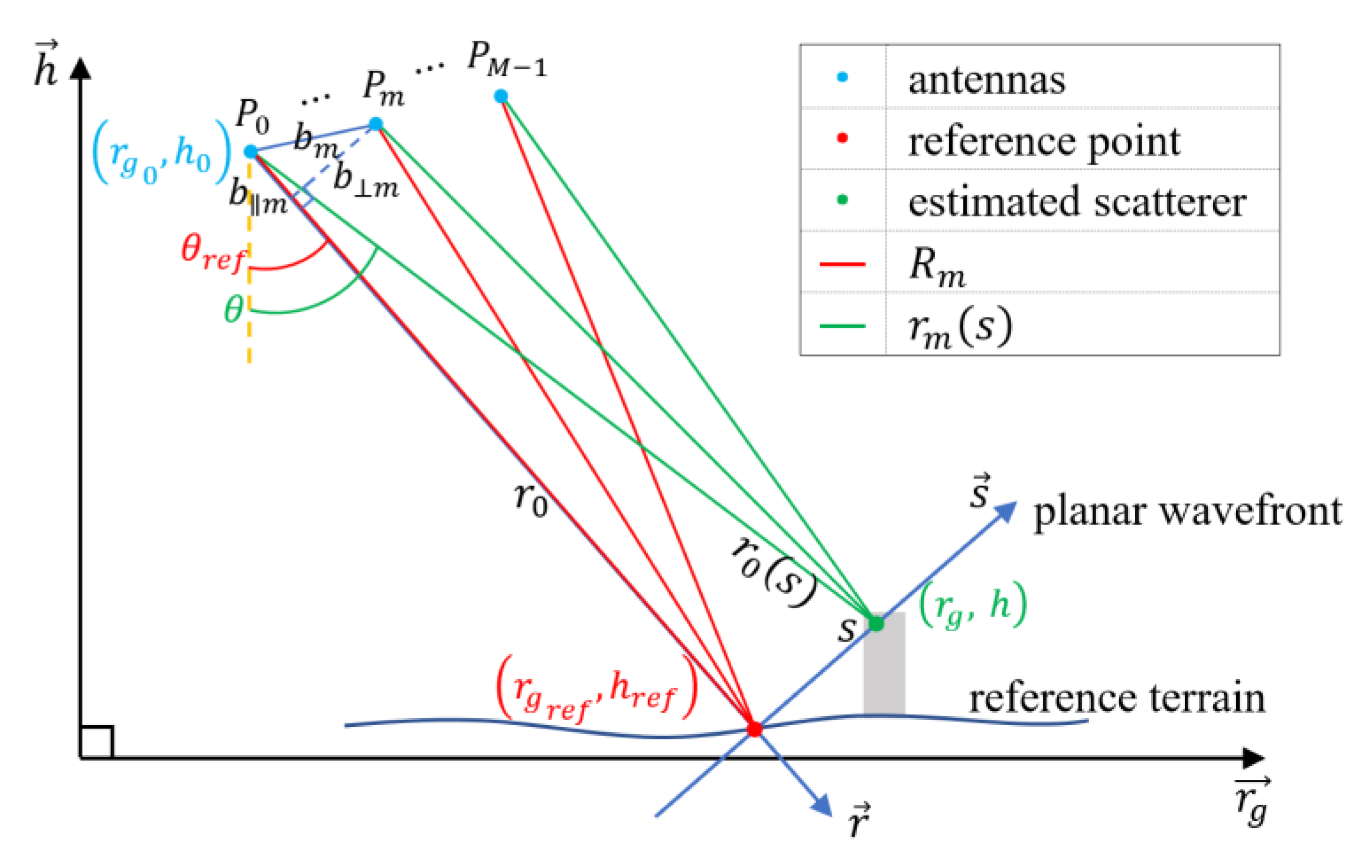
In previous studies [5,10,15], on account of the large slant range from antennas to scatterers, scatterers in the same azimuth–range cell are assumed to be distributed on a planar wavefront. In conventional TomoSAR geometric model, the reference terrain is essential to obtain the reference line of sight (LOS) at each range cell. Then, the planar wavefront is normal to the LOS. As shown in Figure 1, the intersection of the planar wavefront and the LOS is termed the reference point in this paper. The slice line on the planar wavefront at the azimuth sample is denoted as the elevation axis with the reference point as the origin, and the LOS is denoted as the range axis. The rectangular coordinate form of the radar frame is composed of these axes [16]. Indeed, radar receives echoes from scatterers on the same spherical wavefront at the same time, and scatterers in the same azimuth–range cell should be assumed to be distributed on a spherical wavefront. The gap between the planar wavefront and the spherical wavefront will increase with the decrease of the slant range.
In recent years, many high-resolution data have been acquired from platforms other than satellites and airplanes flying at high altitude, such as low-altitude airplanes and unmanned aerial vehicles (UAV) [17]. In contrast to the spaceborne and high-altitude airborne cases, the slant range from the sensor to the observed scene is shorter in low-altitude airborne and UAV-borne cases. It will result in a greater degree of separation between the planar wavefront and the spherical wavefront, especially at the boundary of the illuminated region away from the reference terrain in the elevation direction, as the red arrow in Figure 1. The distance between an estimated scatterer on a planar wavefront and the corresponding scatterer on a spherical wavefront may be larger than one range resolution cell, which results in the conventional TomoSAR imaging model no longer being interpretable in this case. By modifying the conventional TomoSAR imaging model, we propose a TomoSAR imaging model based on the spherical wavefront geometry. The area where scatterers are located is changed from a planar wavefront to a spherical wavefront in the TomoSAR imaging geometry. In the new model, the reflectivity function in the third dimension will refer to off-nadir angle rather than elevation. The pixel’s formula changes from a line integral to an integral along the arc of a circle. The slant range from antennas to scatterers is reformulated and the geodetic coordinate transform is changed.
In the conventional model based on the planar wavefront geometry, the Fourier transform form of a pixel is attributed to some approximation of the slant range [10,18]. To visualize and quantify the effect of these approximations on the reconstruction of the illuminated scene, we derive the approximation procedure and construct some new TomoSAR imaging models using the exact and approximated formulas of the slant range from antennas to scatterers on a planar wavefront. We denote these models as planar wavefront models. When the compressed sensing method is introduced into the TomoSAR field, it is not necessary to approximate the formula of the slant range and obtain the Fourier transform form of the reflectivity function in the third dimension. Therefore, in our model based on a spherical wavefront geometry, the formula of the slant range is the exact distance between antennas and scatterers on a spherical wavefront. In order to compare it with planar wavefront models with approximated formulas of the slant range, we also derive the approximated formula of the distance between antennas and scatterers on a spherical wavefront, and we construct a new model using this formula. We denote these models as spherical wavefront models.
In this paper, TomoSAR imaging models based on a planar wavefront geometry or a spherical wavefront geometry and with different formulas of slant range are derived in detail, and we propose transformations between some of these models. Results obtained from experiments on simulated data and measured data verify the effectiveness of the spherical wavefront models and transformations we proposed. The findings in this paper will benefit the study of TomoSAR in low-altitude cases. This paper is organized as follows. In Section 2, planar wavefront models and spherical wavefront models are introduced in detail. We explore the relationship between planar wavefront models and spherical wavefront models, and we provide two transformation methods. In Section 3, experimental results based on simulated data and real data under different models are presented and quantitatively analyzed. A discussion and conclusions are given in Section 4 and Section 5, respectively.

2. TomoSAR Imaging Models

The TomoSAR imaging model consists of three parts:
  • The distribution of scatterers. There are two kinds of distributions. One is a straight-line distribution and the other is an arc-line distribution;
  • The formulas of the range between antennas and scatterers and the expression of the value of the 2-D SAR image. Regarding the former, for different scatterer distributions, there are different range formulas, and these formulas will lead to different approximate forms. As for the latter, the expression is formed in the radar frame. For the straight-line distribution, the radar frame is in rectangular coordinate system. For the arc-line distribution, the radar frame is in polar coordinate system;
  • The geodetic coordinate transformation method. Because the expression of the value of the 2-D pixel is formed in the range-azimuth plane, the inversion results should be transformed into the geodetic coordinate system to be more intuitive.
In total, there are six models mentioned in this paper, as shown in Table 1, of which four models are constructed based on the planar wavefront and different range formulas, and two models are constructed based on the spherical wavefront and different range formulas. To facilitate the representations of different models, we will number these models from 1 to 6, and superscript is used in the formula to indicate which variable belongs to which model.

2.1. Planar Wavefront Models

As shown in Figure 2, we only consider the ground range–height plane of an azimuth sample position and assume all targets are isotropic point-like scatterers for the sake of convenience. The mode of tomography is single pass with an antenna array with M antennas at positions P 0 ,   P 1 ,   ,   P M 1 , and we set antenna P 0 as the master antenna. Assume that these antennas are colinear but not necessarily uniform, which is common in practice. There are two coordinate systems, one is called ground frame and is made up of the ground range r g and the height h (perpendicular to the ground range), and the other is called radar frame and is made up of the slant range r and elevation s (normal to the LOS) [13]. r 0 is the distance between the master antenna and the center of the pixel at the same azimuth position, and r 0 is also the minimum distance from master antenna to the planar wavefront in the planar wavefront geometry,
r 0 = r start + ( n r 1 ) ρ r
where r start is the slant range at the near end of the SAR image obtained by the master antenna, n r is the range index of the pixel in the SAR image, and ρ r is the length of a range cell. r 0 is also denoted as the distance between the master antenna and the reference terrain.
Assume the 2-D images obtained from each antenna are properly co-registered and the phase of each pixel depends only on the scattering property of the scatterer and the distance between the corresponding antenna and the scatterer. That is to say, the amplitude and phase calibration have been conducted in advance. Then, the measurement vector g contains the values of the image sets of the same pixel and the m th element can be expressed as [18].
g m = L 2 L 2 γ ( i ) ( s ) exp ( j 2 π 2 r m ( i ) ( s ) λ ) d s ,       m = 0 , , M 1 ; and   i = 1 , 2 , 3 , 4
where L is the length of integral interval, γ ( i ) ( s ) is the reflectivity function along elevation s , λ is the operating wavelength in i th model, and r m ( i ) ( s ) is the distance from m th antenna to the scatterer at elevation s in i th model.
In model 1, using the exact form of the range between antennas and scatterers, r m ( 1 ) ( s ) can be represented as [18].
r m ( 1 ) ( s ) = ( r 0 b m ) 2 + ( s b m ) 2 ,
where
b m = b m sin ( θ r e f α m ) ,
b m = b m cos ( θ r e f α m ) ,  
b m is the length of m th baseline corresponding to the connecting line between m th antenna and the master antenna; b m is the projection length of m th baseline on the connecting line between the master antenna and the reference terrain, i.e., the reference LOS of the master antenna; b m is the distance from the m th antenna to that connecting line; θ r e f is the off-nadir angle of the reference LOS; and α m is the baseline inclination of m th baseline.
In model 2 to 4, different approximate forms of the range between antennas and scatterers are used. In the early days of the TomoSAR field, spectral analysis was often used for inversion. Therefore, Equation (3) is usually approximated to become the form of Fourier transform. From (3), we have
r m ( 1 ) ( 0 ) = ( r 0 b m ) 2 + b m 2 ,
and we let R m = r m ( 1 ) ( 0 ) represent the range between the m th antenna and the reference point. Subsequently, we substitute R m back into (3) and get
r m ( 1 ) ( s ) = R m 2 + s 2 2 b m s .
It should be noticed that
r 0 = R 0 = r 0 ( 0 ) ,
which means that the slant range of a pixel in the SAR image obtained from the master antenna, the distance between the master antenna and the reference point, and the slant range from the master antenna to a scatterer at 0 m elevation are equal.
Based on the 1st Taylor approximation with respect to ( s 2 2 b m s ) , Equation (7) can be converted to
r m ( 1 ) ( s ) = R m 2 + s 2 2 b m s R m + s 2 2 b m s 2 R m = R m + s 2 2 R m b m R m s .
Then, the formula of the slant range in model 2 is
r m ( 2 ) ( s ) = R m + s 2 2 R m b m R m s .
Compared with the exact form (3), this is a relatively accurate approximation and basically does not affect the inversion results, which will be verified in Section 3. But this approximation is always followed by another further approximation
r m ( 3 ) ( s ) = R m + s 2 2 r 0 b m R m s .
It seems that R m r 0 , but this approximation will affect the inversion results in the low-height airborne case. The goal of these approximations is that researchers want to transform the exam form of the planar wavefront model into the Fourier form. Therefore, the formula of r m ( 3 ) ( s ) in (11) should be divided into three parts. The first part only depends on positions of antennas, and this part can be eliminated by the so-called deramping operation [10]. The second part depends on the position of scatterer, and this part can be compensated by postprocessing. The third part is the coupling term of the variable which refers to the positions of antennas and the variable which refers to the position of the scatterer, and this part plays the role of Fourier base. The second term in (11) only affects the phase of the inversion results and can be temporarily ignored. Then, r m ( i ) ( s ) becomes
r m ( 4 ) ( s ) = R m b m R m s ,
which is equal to the first-order Taylor expansion of r m ( 1 ) ( s ) at s = 0 .
For these planar wavefront models, transformation relations from the radar frame to the ground frame are
{ r g = r g r e f + s cos ( θ r e f ) h = h r e f + s sin ( θ r e f ) ,
where r g and h denote the ground range and height of the scatterer. θ r e f is the off-nadir angle of the reference LOS. r g r e f and h r e f denote the ground range and height of the reference point, and can be expressed as
{ r g r e f = r g 0 + r 0 sin ( θ r e f ) h r e f = h 0 r 0 cos ( θ r e f ) ,
where r g 0 and h 0 denote the ground range and height of the master antenna.
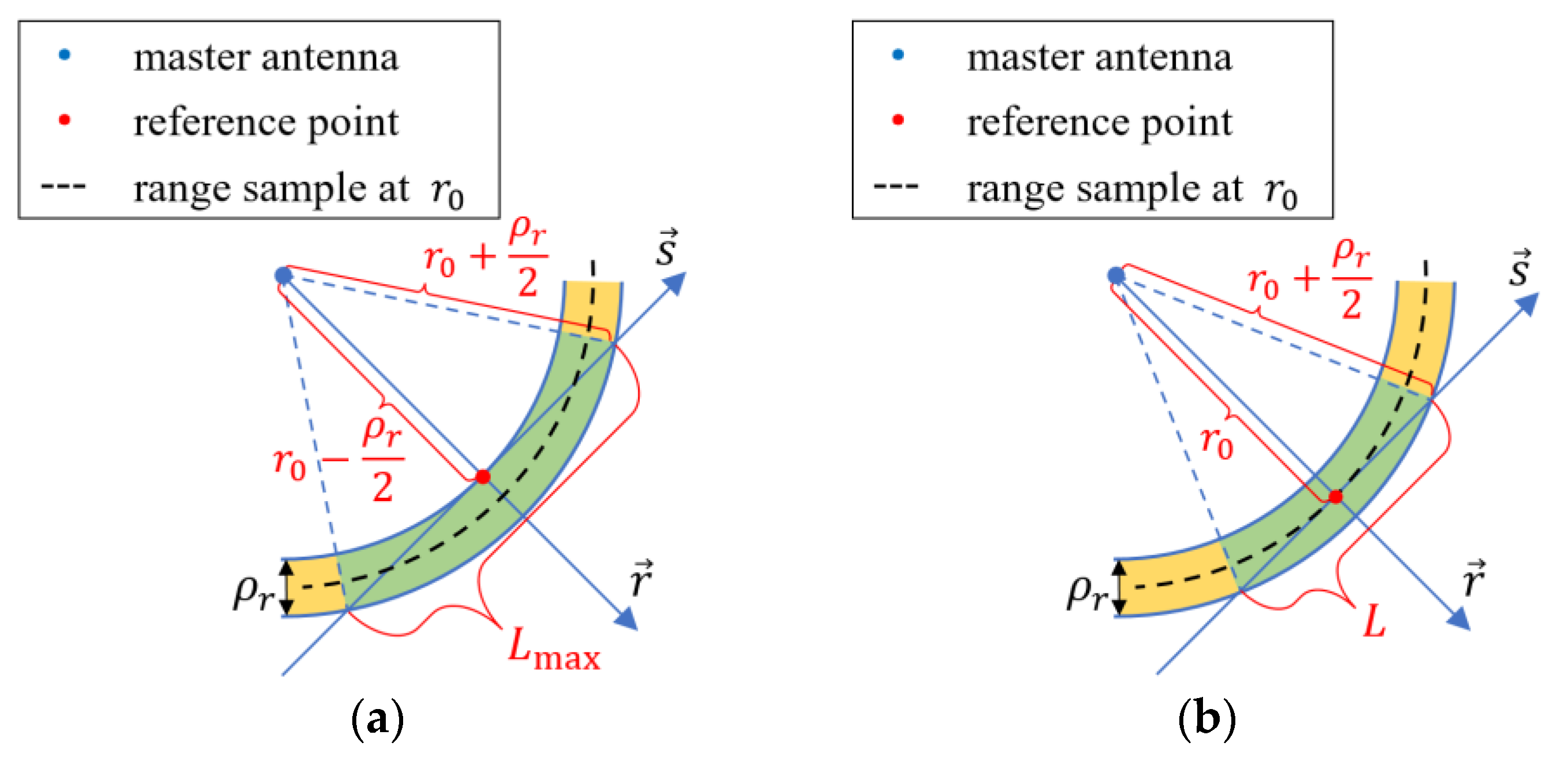
The conventional TomoSAR model chooses a one-line segment in each pixel as the reference inversion area, i.e., the part where the elevation axis coincides with the spherical wavefront, and denotes it as elevation axis s . The center of the line segment is located on the reference terrain and denoted as the origin of the elevation axis. The maximum length L max (see Figure 3a) of the line segment is limited by the range and the range resolution
L max = 2 ( r 0 + ρ r 2 ) 2 ( r 0 ρ r 2 ) 2
However, most studies choose the origin of the elevation axis in the center of the pixel, so the length L (see Figure 3b) of the line segment is
L = 2 ( r 0 + ρ r 2 ) 2 r 0 2 .
Nevertheless, in the low-height airborne and UAV-borne cases, L is similar with L max and both are usually smaller than the length of the extension of the illuminated scene, which is mentioned in Section 3.1. As shown in Figure 3, when a scatterer in the resolution cell is not located on the elevation axis, there are two cases. In the first case, the scatterer may be located in the green area, except the elevation axis. The assumption that scatterers are located on a planar wavefront is reasonable. In the second case, the scatterer may be located in the yellow area. The elevation axis no longer overlaps with the resolution cell. The planar wavefront assumption no longer holds, and the geodetic transform is in (13). In Section 2.4, transformation between models is proposed to solve this problem.

2.2. Spherical Wavefront Models

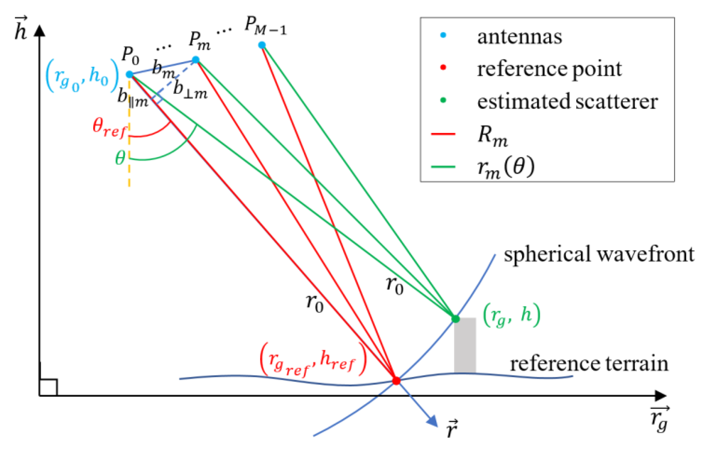
In order to solve the problem that the integral interval of the planar wavefront models can not cover the distribution region of scatterers in the low-height airborne case, we choose one arc line at the center of the pixel as the reference inversion area, as shown in Figure 4. r 0 is the distance from the master antenna to the center of the pixel at the same azimuth position, and all scatterers on the same spherical wavefront have the same distance from the master antenna. Subsequently, the pixel g m can be represented as the circular integral about the off-nadir angle θ rather than as a linear integral about the elevation s
g m = θ min ( r 0 ) θ max ( r 0 ) γ ( i ) ( θ ) exp ( j 2 π 2 r m ( i ) ( θ ) λ ) d θ   m = 0 , , M 1 ; and   i = 5 , 6
where θ min ( r 0 ) and θ max ( r 0 ) are the minimum and maximum off-nadir angles of the illuminated scene at slant range r 0 , respectively. γ ( i ) ( θ ) is the reflectivity function related to the off-nadir angle θ in i th model, and r m ( i ) ( θ ) is the distance between the m th antenna and the scatterer with off-nadir angle θ in i th model.
In model 5, the exact form of the range is
r m ( 5 ) ( θ ) = ( r 0 sin ( θ α m ) b m ) 2 + ( r 0 cos ( θ α m ) ) 2 = r 0 2 + b m 2 2 b m r 0 sin ( θ α m ) .
Compared with (3), (10), (11) and (12), the advantages of this model are not only the extension of the inversion region, but also that there is no need for the reference terrain.
Although the approximate expansion of the model is no longer necessary under the compressed sensing method, Taylor expansion is also carried out here to compare with the approximate form of the conventional model based on the planar wavefront geometry. We use R m to denote the distance from m th antenna to the reference terrain
R m = r m ( 5 ) ( θ r e f ) = r 0 2 + b m 2 2 b m r 0 sin ( θ r e f α m ) ,
and substitute it into Equation (18). After first-order Taylor expansion with respect to ( sin ( θ α m ) sin ( θ r e f α m ) ) , we have
r m ( 5 ) ( θ ) = R m 2 2 b m r 0 ( sin ( θ α m ) sin ( θ r e f α m ) ) R m 2 b m r 0 ( sin ( θ α m ) sin ( θ r e f α m ) ) 2 R m .
Then, the formula of the slant range in model 6 is
r m ( 6 ) ( θ ) = R m b m r 0 R m ( sin ( θ α m ) sin ( θ r e f α m ) ) ,
For these spherical wavefront models, transformation relations from the radar frame to the ground frame are
{ r g = r g 0 + r 0 sin ( θ ) h = h 0 r 0 cos ( θ )

2.3. Discretization of Models

The continuous-space system models can be approximated by discretizing the continuous-reflectivity function along s , or refer to θ . We assume that there are only a few scatterers in each pixel, and the point spread functions of these scatterers are delta functions. Then, the formula of the pixel can be approximated from the integral about the scattering distribution function as the sum about the backscattering coefficients of several scatterers. In order to unify the discretization processing of models and the quantitative analysis of results by planar wavefront models and spherical wavefront models, we transform elevation s in planar wavefront models to off-nadir angle θ using
s = r 0 tan ( θ θ r e f ) .  
These models become
g m = k = 1 K γ k ( 1 ) exp ( j 2 π 2 λ ( r 0 b m ) 2 + ( r 0 tan ( θ k ( 1 ) θ r e f ) b m ) 2 ) ,   m = 0 , , M 1
g m = k = 1 K γ k ( 2 ) exp ( j 2 π 2 λ ( R m + ( r 0 tan ( θ k ( 2 ) θ r e f ) ) 2 2 R m b m R m r 0 tan ( θ k ( 2 ) θ r e f ) ) ) ,   m = 0 , , M 1
g m = k = 1 K γ k ( 3 ) exp ( j 2 π 2 λ ( R m + ( r 0 tan ( θ k ( 3 ) θ r e f ) ) 2 2 r 0 b m R m r 0 tan ( θ k ( 3 ) θ r e f ) ) ) ,   m = 0 , , M 1
g m = k = 1 K γ k ( 4 ) exp ( j 2 π 2 λ ( R m b m R m r 0 tan ( θ k ( 4 ) θ r e f ) ) ) ,   m = 0 , , M 1
g m = k = 1 K γ k ( 5 ) exp ( j 2 π 2 λ ( r 0 2 + b m 2 2 b m r 0 sin ( θ k ( 5 ) α m ) ) ) ,   m = 0 , , M 1
g m = k = 1 K γ k ( 6 ) exp ( j 2 π 2 λ ( R m b m r 0 R m ( sin ( θ k ( 6 ) α m ) sin ( θ r e f α m ) ) ) ) ,   m = 0 , , M 1
The objective of TomoSAR is to retrieve θ k ( i ) and γ k ( i ) for each azimuth–range pixel, and the compressed sensing method can solve this inverse problem. These discrete models can be represented as [19]
g = R ( i ) γ ( i ) ,   i = 1 , 2 , 3 , 4 , 5 , 6
where g is the measurement vector with M elements g m , i is the model’s number, R ( i ) is an M × N mapping matrix with R m n ( i ) = exp ( j 2 π 2 r m ( i ) ( θ n ) / λ ) , and γ ( i ) is the discrete reflectivity vector with N elements γ n = γ ( θ n ) . θ n   ( n = 1 , ,   N ) denotes the discrete off-nadir angles. There are many algorithms to solve the inversion problem (30), but it is not the focus of this article and will not be discussed here.

2.4. Transformation between Models

By analyzing the experimental results and expressions of each model, we find some transformation relations between these models and propose two transformation methods, which can convert the results of the poorly performing model based on the planar wavefront into the results of the model based on the spherical wavefront. In this section, we first give out the transformation relation from the exact form of the planar wavefront model to the exact form of the spherical wavefront model. Then, the transformation relation from the approximate form of the planar wavefront model to the approximate form of the spherical wavefront mode is discussed.
Although there are errors on geodetic coordinates of scatterers produced by the exact form of the planar wavefront model as shown in Section 3.1.3, the off-nadir angle of estimated scatterers is nearly accurate. This also confirms that the tomography processing is sensitive to the off-nadir angle of the scatterer but cannot distinguish the offset of the scatterer in the range direction. It is easy to see that we keep the off-nadir angle obtained by the exact form of the planar wavefront model and abandon the geodetic coordinate transformation method corresponding to this model, but use the geodetic coordinate transformation method (13) corresponding to the spherical wavefront model. Then, the transformed ground range r g and height h of the scatterer are
{ r g = r g 0 + r 0 sin ( θ ( 1 ) ) h = h 0 r 0 cos ( θ ( 1 ) )  
From the experimental result shown in Section 3.1.3, the phase of scatterers on the reference terrain is flat, but the phase of the other scatterers is rambling, which should be corrected in applications which depend on the signal phase characteristics. We assume that the scatterers are distributed at the center of the pixel, i.e., the arc line considered as the reference inversion area in the spherical wavefront model. Phase correction is to compensate for the effect of the distance difference between the segment line in model 1 and the arc line in model 5. Both model 1 and model 5 deal with the same pixel, so
k = 1 K γ k ( 1 ) exp ( j 2 π 2 λ r m ( 1 ) ( θ k ) ) = k = 1 K γ k ( 5 ) exp ( j 2 π 2 λ r m ( 5 ) ( θ k ) ) ,   m = 0 , , M 1
And we assume that the amplitude of scatterers can be inversed correctly under both model 1 and model 5
| γ k ( 1 ) | = | γ k ( 5 ) | ,     k = 1 , , K
which will be verified in Section 3.1. To be honest, the next step is not very rigorous. We try to prove the universality of the transformation obtained through this derivation process in Section 3.1. We presume that
γ k ( 1 ) exp ( j 2 π 2 λ r m ( 1 ) ( θ k ) ) γ k ( 5 ) exp ( j 2 π 2 λ r m ( 5 ) ( θ k ) ) ,     k = 1 , , K   and   m = 0 , , M 1
therefore,
γ k ( 5 ) γ k ( 1 ) exp ( j 2 π 2 λ ( r m ( 1 ) ( θ k ) r m ( 5 ) ( θ k ) )   ) ,     k = 1 , , K   and   m = 0 , , M 1
meaning that
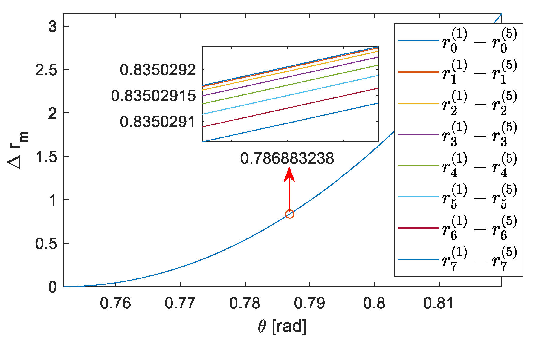
r i ( 1 ) ( θ k ) r i ( 5 ) ( θ k ) r j ( 1 ) ( θ k ) r j ( 5 ) ( θ k ) ,     i j   and   i , j = 0 , , M 1
which can be verified by the numerical experiment, and the difference between r m ( 1 ) ( θ ) r m ( 5 ) ( θ ) with different m is minimal as shown in Figure 5. Eventually, the transformed reflectivity γ ( 1 ) ( θ ) can be represented as
γ ( 1 ) ( θ ) = γ ( 1 ) ( θ ) exp ( j 2 π 2 λ ( r 0 ( 1 ) ( θ ) r 0 ( 5 ) ( θ ) )   ) .
The transformation relation between the approximate form of the planar wavefront model and the spherical wavefront model is more difficult. Here we define a new coordination system named the baseline coordinate system, as shown in Figure 6 by the red solid line. The origin is the position of the master antenna, the abscissa axis denoted as n is the direction normal to the baseline direction, and the vertical axis denoted as b is the baseline direction. It is worth noting that it is based on the assumption that the antennas are collinear. Then, we represent the ordinate of the scatterer and the reference point as b and b r e f , respectively.
Model 4 is represented in the radar coordinate system in rectangular form, and model 6 is represented in the radar coordinate system in polar form. Next, we transform them into the baseline coordinate system. The relation between elevation s and b in model 4 is
s k ( 4 ) = b k ( 4 ) b r e f cos ( θ r e f α )
In Section 2.3, the elevation s k ( 4 ) of k th scatterer has been transformed into a formula which refers to off-nadir angle θ k ( 4 )
s k ( 4 ) = r 0 tan ( θ k ( 4 ) θ r e f )
Then, considering (5), (38), (39), model 4 in the discrete form (27) becomes
g m = k = 1 K γ k ( 4 ) exp ( j 2 π 2 λ ( R m b m R m ( b k ( 4 ) b r e f ) ) ) ,   m = 0 , , M 1
The relation between off-nadir angle θ and b in model 6 is
r 0 sin ( θ k ( 6 ) α ) = b k ( 6 )
r 0 sin ( θ r e f ( 6 ) α ) = b r e f ( 6 )
Then, the discrete version of model 6 in (29) becomes
g m = k = 1 K γ k ( 6 ) exp ( j 2 π 2 λ ( R m b m R m ( b k ( 6 ) b r e f ) ) ) ,   m = 0 , , M 1
From (40) and (43) we can see that model 4 and model 6 are the same in the baseline frame, so we can get
b k ( 4 ) = b k ( 6 ) .
γ k ( 4 ) = γ k ( 6 )
Using (38), (39), (41), (42) and (44), we can get the relation of the off-nadir angle of the scatterer in model 4 and model 6
θ k ( 6 ) = asin ( sin ( θ k ( 4 ) α ) cos ( θ k ( 4 ) θ r e f ) ) + α ,
so that the transformed off-nadir angle θ ( 4 ) of scatterers can be expressed as
θ k ( 4 ) = asin ( sin ( θ k ( 4 ) α ) cos ( θ k ( 4 ) θ r e f ) ) + α .
Then, the transformed ground range r g and height h of the k th estimated scatterer are
{ r g = r g 0 + r 0 sin ( θ k ( 4 ) ) h = h 0 r 0 cos ( θ k ( 4 ) )  

3. Experiments and Results

3.1. Experiments on Simulated Data

In this subsection, 3-D reconstructions of illuminated scenes which resulted from processing simulated data with different TomoSAR imaging models are analyzed. Two experiments are designed with different simulated scenarios. In experiment 1, in order to get a better reconstruction of the illuminated scene, we develop a simulated scenario where scatterers have the same amplitude and phase of reflectivity. In experiment 2, a simulated scenario where scatterers have different amplitudes and phases of reflectivity, is constructed to verify the universality of the transformation between model 1 and model 5.

3.1.1. Simulated Dataset

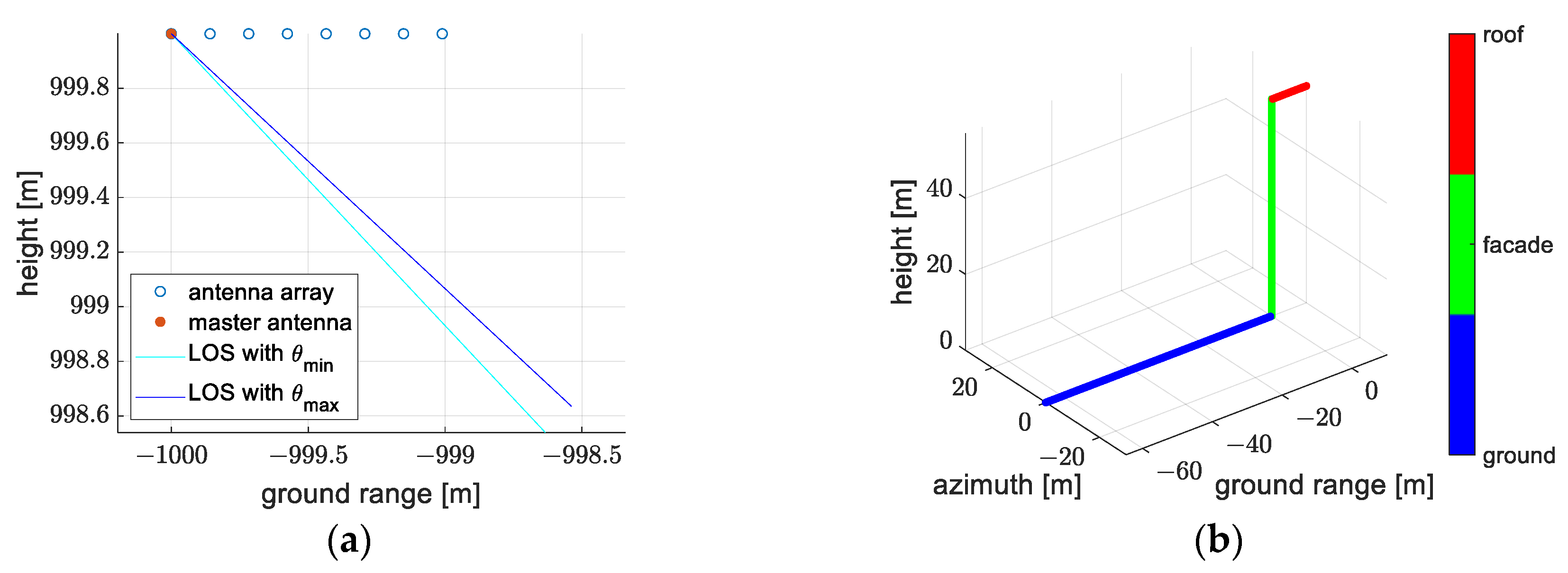
We simulated eight 2-D SAR images corresponding to different trajectories, which are isometry and coplanar. The configuration of the antenna array and the structure of the simulated scene are shown in Figure 7. The scene is composed of a ground at 0 m height, a vertical façade at 0 m ground range and a roof at 57.0524 m height, resulting in layover areas with different sparsity in the SAR images. The reference terrain is a 0 m ground plane, which can be used in models 1, 2, 3, 4 and 6. More details about the system configuration and the illuminated scene are listed in Table 2.
For the sake of computational efficiency, we simulate only one scatterer in azimuth direction, and slice a line containing scatterers in the stack of SAR images to perform tomographic processing. In order to better calculate the inversion error of scatterers, every scatterer is located on the sampling grids in both azimuth direction and range direction. By this means, there will be no error between simulated scatterers and estimated scatterers in the azimuth and range directions. We only need to analyze the error between them in ground range and height direction.
Referring to Equation (16), the length L of the effective integral interval under the planar wavefront models is about 37 m and 37.61 m at the near and far ends of the illuminated scene, respectively. Referring to Equation (15), the maximum length L max of the effective integral interval under the planar wavefront models is 52.33 m and 53.18 m at the near and far ends of the illuminated scene, respectively. The height of the scene is about 57 m and the off-nadir angle of the center of the scene is about 45°. Therefore, the extension in the elevation direction is about 81 m. The lengths L and L max are smaller than the length of the extension of the illuminated scene.
In experiment 1, all the simulated scatterers have the same amplitude and phase as shown in Figure 8. The phase and amplitude of scatterers are 1 and 0 rad, respectively. For convenience, the amplitude of the scatterer in this paper has no dimension. In this experiment, we focus more on the locations of scatterers reconstructed under different models and transformed models, and we only consider whether the amplitude and phase of estimated scatterers are constant to analyze the accuracy of inversion. It is meaningless to determine whether the amplitude and phase of the inversed results are the same as the true value exactly due to the effect of 2-D SAR imaging.
For experiment 2, the simulated scenario is shown in Figure 9. The amplitude and phase of scatterers on the roof are 2 and π / 2   rad, respectively. The amplitude and phase of scatterers on the façade are 3 and 0 rad, respectively. The amplitude of scatterers on the ground is 1 and their phase is random from π rad to π rad. In this experiment, the effectiveness of the transformation between model 1 and model 5 in a more complex scenario will be verified.

3.1.2. Evaluation Metrics

In order to quantitatively analyze the experimental results, some evaluation metrics are introduced in the experiments. The mean error (ME) is used to evaluate the average deviation between estimated and simulated scatterers in ground range and height directions. The root mean squared error (RMSE) can reflect the uniformity degree of the deviation. The expressions of ME and RMSE on the ground range and height are given here,
ME r g = j = 1 Q ( r g ^ j r g j ) Q ,
RMSE r g = j = 1 Q ( r g ^ j r g j ) 2 Q ,
ME h = j = 1 Q ( h ^ j h j ) Q ,
RMSE h = j = 1 Q ( h ^ j h j ) 2 Q ,
where Q is the number of the estimated scatterers; r g ^ j and h ^ j are the ground range and height of j th estimated scatterer, respectively; and r g j and h j are the ground range and height of the simulated scatterer corresponding to the j th estimated scatterer, respectively. The smaller these four metrics are, the higher the position estimation accuracy of the scatterers is.
Due to the effect of 2-D SAR imaging on the amplitude of scatterers and the nearly constant phase bias, it is hard to compensate the amplitude and phase. We directly calculate the sample mean and standard deviation of the phase error and amplitude of estimated scatterer.
Δ ϕ j = arg ( γ ^ j γ j ) ,   j = 1 , , Q
μ Δ ϕ = j = 1 Q Δ ϕ j Q
σ Δ ϕ = j = 1 Q ( Δ ϕ j μ Δ ϕ ) 2 Q 1
A j = | γ ^ j | ,   j = 1 , , Q
μ A = j = 1 Q A j Q
σ A = j = 1 Q ( A j μ A ) 2 Q 1
where γ ^ j is the reflectivity of the j th estimated scatterer and γ j is the reflectivity of the simulated scatterer corresponding to the j th estimated scatterer. Δ ϕ j and A j are the phase error and amplitude of the j th estimated scatterer, respectively. The more similar the μ Δ ϕ of all parts in the simulated building are, the more accurate the estimated phase is. The smaller σ Δ ϕ is, the more accurate the estimated phase is. The estimated amplitude proportions of each part of the building should be consistent with the simulated amplitude proportions, and σ A needs to be an order of magnitude smaller than μ A to ensure the stability of the estimated amplitude.

3.1.3. Results of Experiment 1

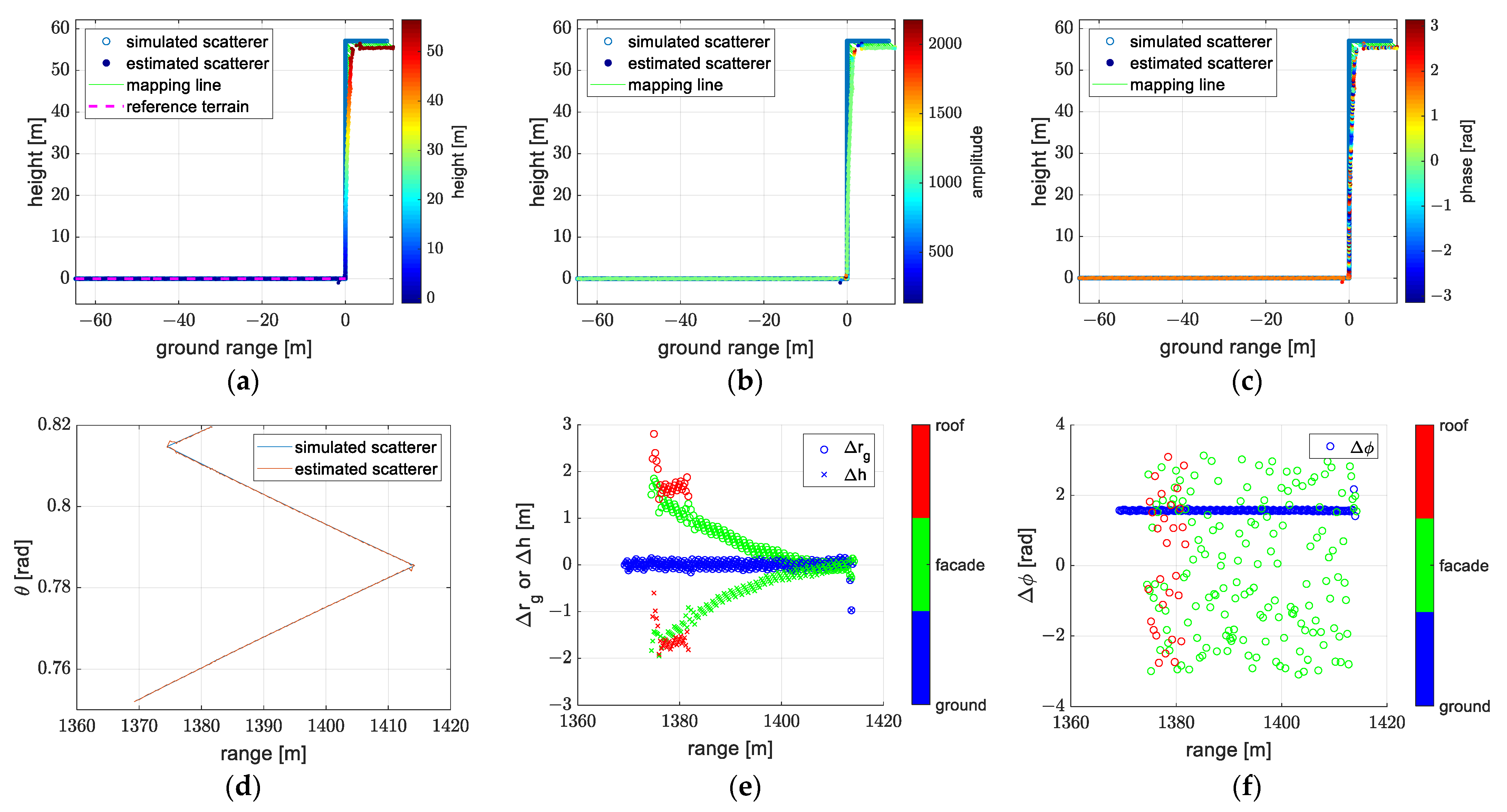
Under model 1 in (24) (the exact form of the planar wavefront model) and model 2 in (25) (the first approximate form of the planar wavefront model), the inversion results and error analysis are presented in Figure 10 and Figure 11, respectively. Results from these two models are very similar, which shows that the approximation in (10) is very accurate. Model 2 will not be considered in future analyses. From the mapping lines in Figure 10a, we can see that the farther the scatterer is from the reference terrain, the farther the position of the inversion result is from the simulated scatterer in the direction of the line of sight. Figure 10b shows that the amplitude of the inversion result is flat, which is consistent with the property of the simulation scene, but the phase of the inversion result is not constant when the scatterer is not located at the reference terrain as shown in Figure 10c. Figure 10d shows that the off-nadir angle of the inversion result is consistent with the simulated one, and this provides evidence that TomoSAR can only distinguish scatterers with different off-nadir angles and is insensitive to the range of the scatterer. When the scatterer is not located at the reference integral area, i.e., straight line in the planar wavefront model and arc line in the spherical wavefront model, the off-nadir angle of the inversion result will be similar with the one of simulated scatterers. The error of the position of different parts of the building is displayed in Figure 10e. The roof, façade and ground of the building are denoted with red, green and blue colors, respectively. The circle symbol represents the error of the inversion result which refers to the simulated scatterer in the ground range, and the cross symbol indicates the error in the height direction. All the scatterers on the roof are far away from the reference terrain; therefore, the error of the ground range and height is large. The scatterers with small range on the façade are at the top and far away from the reference terrain, so the error is large. The scatterers with large range on the façade are at the bottom and close to the reference terrain, so the error is small. Because the error of the ground range is positive and the error of the height is negative except the scatterers on the ground, the estimated scatterers are located at the bottom right of the simulated scatterers. In Figure 10f, the phase error of different parts of the building is shown. The phase of the estimated scatterers on the ground is flat, but the phase of the estimated scatterers on the roof and façade is rambling.
Regarding model 3 in (26) (the second approximate form of the planar wavefront model) and model 4 in (27) (the third approximate form of the planar wavefront model), inversion results and error analysis are presented in Figure 12 and Figure 13, respectively. They are similar except the phase of the inversion result. Model 3 will not be considered in future analyses. From the mapping lines in Figure 13a, we can see that the farther the simulated scatterer is from the reference terrain, the father the position of the inversion result is from the simulated scatterer in the direction normal to the baseline. Figure 13b,c show that the amplitude and the phase of the inversion results are flat, which is consistent with the properties of the simulation scene. Figure 13d shows that there is a large deviation between the off-nadir angle of the inversion results and the simulation results when the scatterer is not located at the reference integral area. The error of the position of different parts of the building is displayed in Figure 13e. The ground range of all parts of the building is accurate, but there is a large error on the height of the roof and the façade. In Figure 13f, the error in the phase of different parts of the building is shown. The phase of the scatterers is flat.
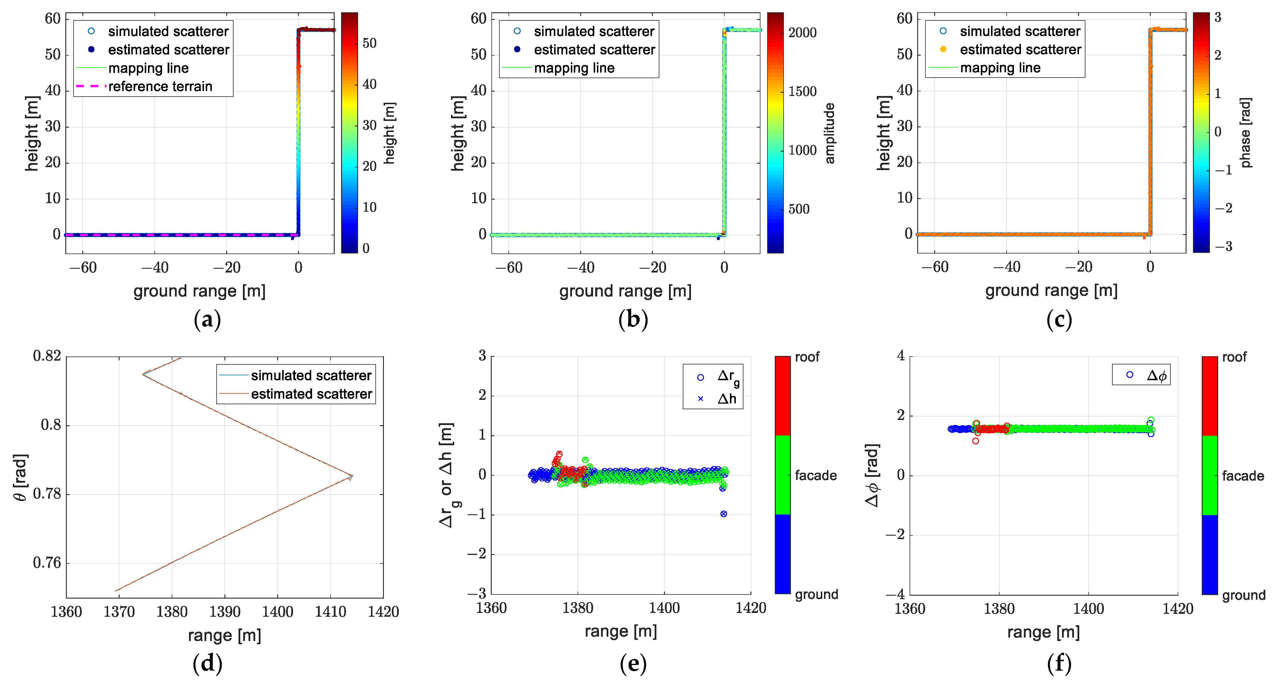
The reconstructions obtained using the exact and approximate forms of the spherical wavefront model are shown in Figure 14 and Figure 15. The results of these two models are generally consistent. We can see that positions of estimated scatterers almost coincide with positions of simulated scatterers, and the amplitude and phase of estimated scatterers are almost constant. The correctness of the spherical wavefront model is proved.
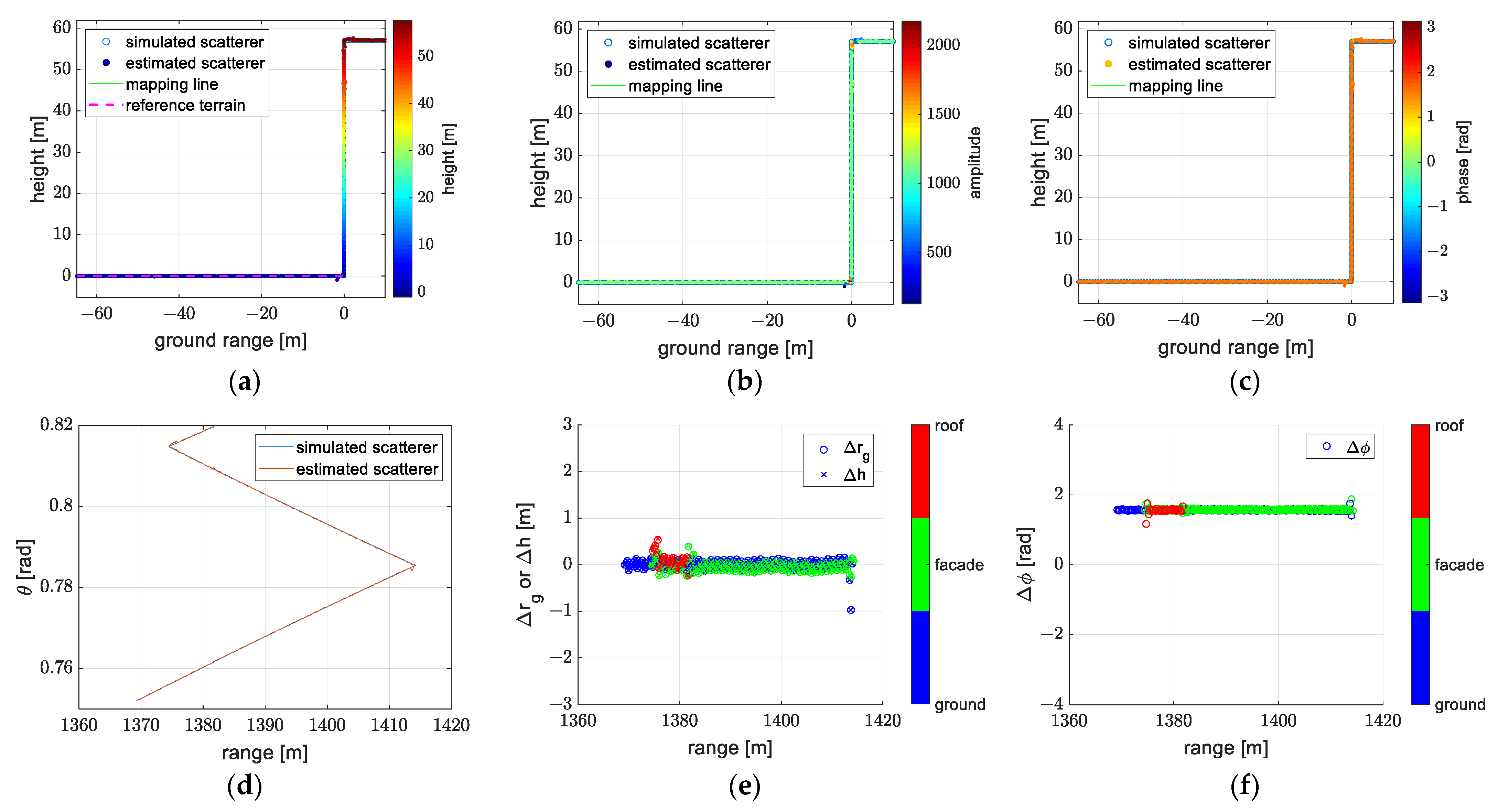
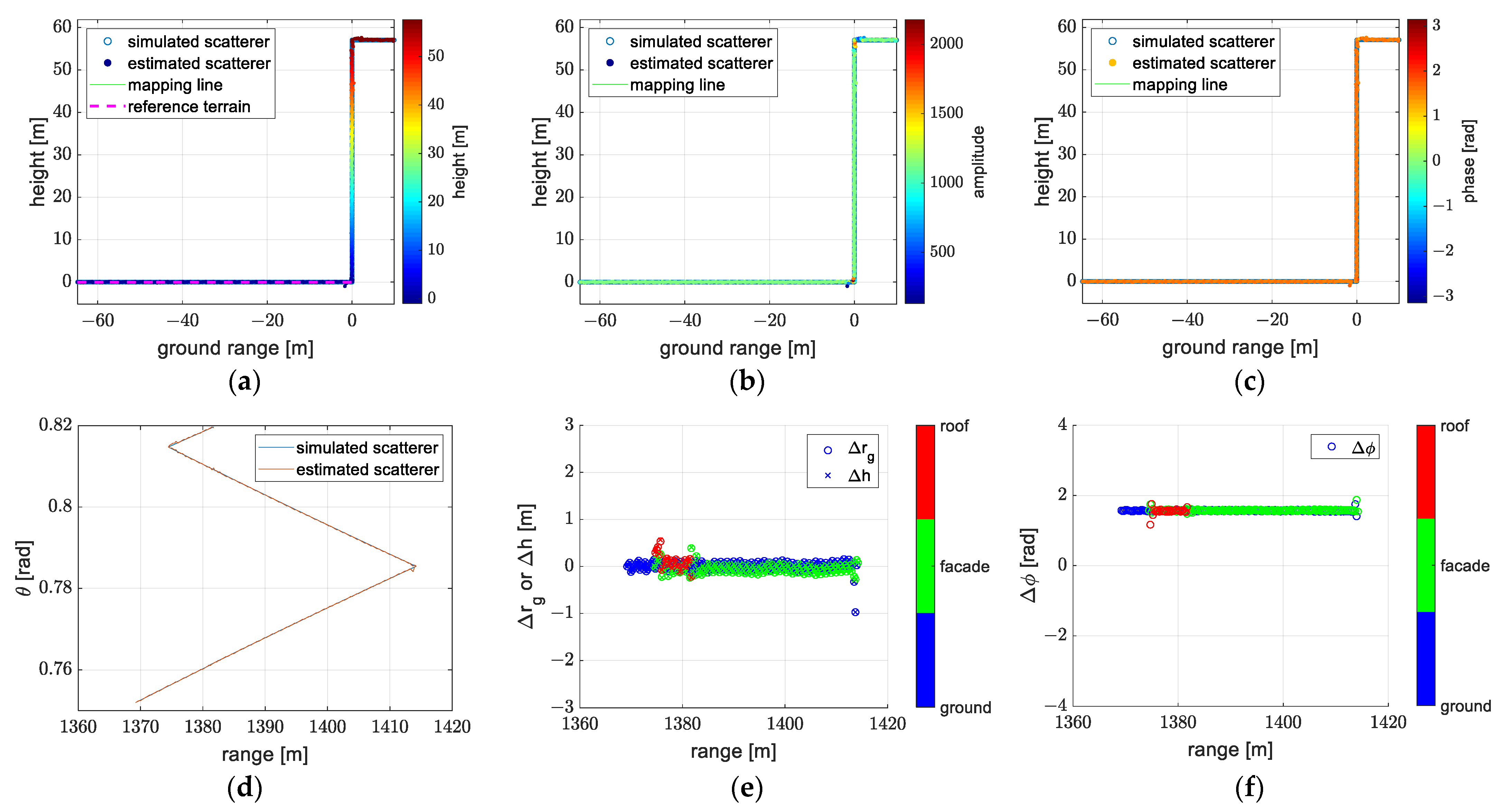
The reconstructions obtained using the exact and approximate forms of the planar wavefront model after transformation are shown in Figure 16 and Figure 17. Figure 14, Figure 15, Figure 16 and Figure 17 are almost the same. The effectiveness of the transformation methods is verified.
To give a comprehensive summary of this subsection, Table 3 shows the quantitative analysis of inversion results using simulated data by different models. In this paper, bold numbers in all tables indicate unqualified results. From this table, the conclusions are drawn that the ground range, height and phase of inversion results under model 1 are inaccurate, and that the height of inversion results under model 4 is inaccurate. After using transformation methods mentioned in Section 2.4, the inversion results under transformed model 1 and transformed model 4 are accurate.

3.1.4. Results of Experiment 2

In this experiment, the amplitude and phase of scatterers on the roof are 2 and π / 2   rad, respectively. The amplitude and phase of scatterers on the façade are 3 and 0 rad, respectively. The amplitude of scatterers on the ground is 1 and their phase is random from π rad to π rad.
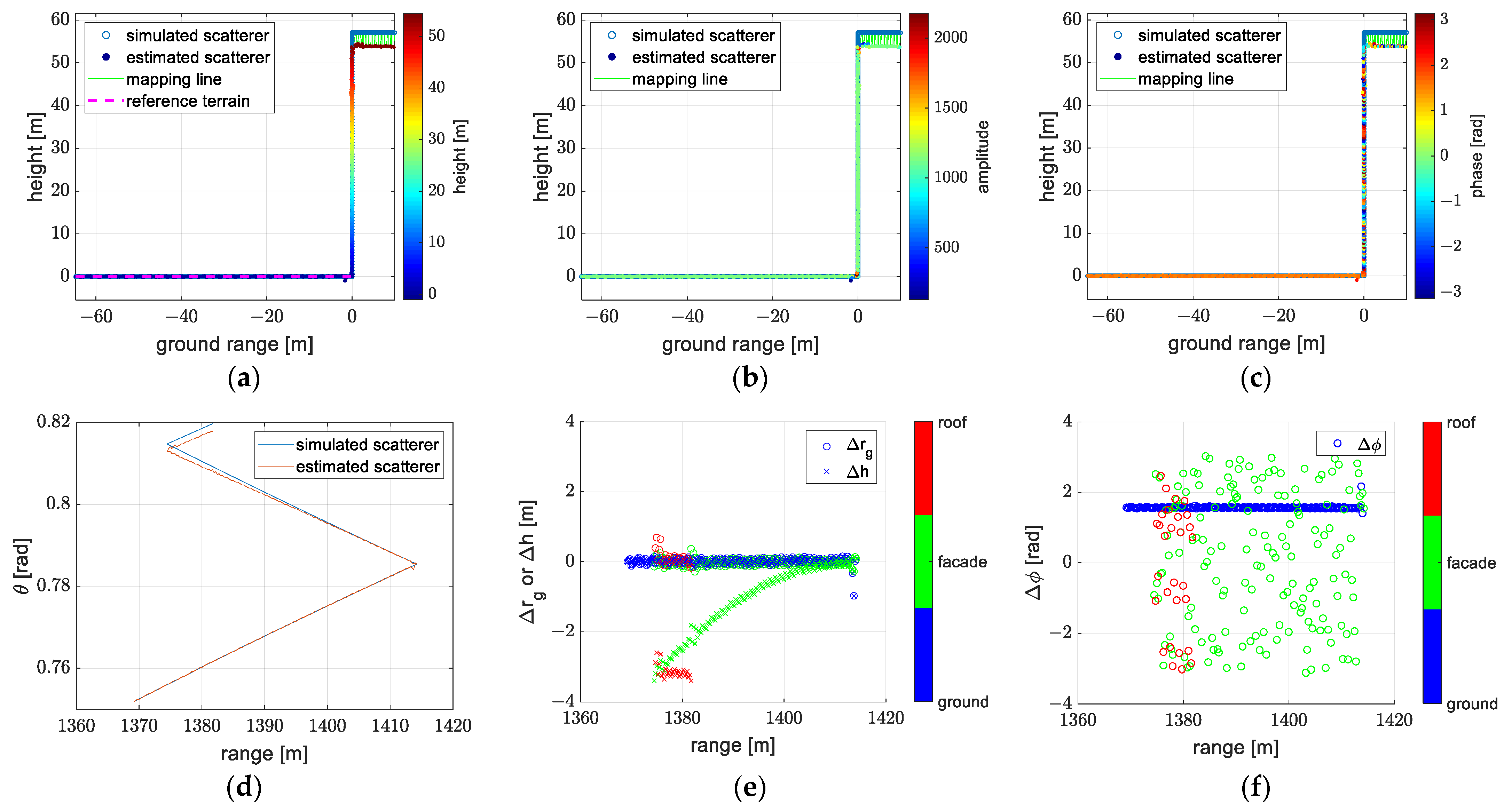
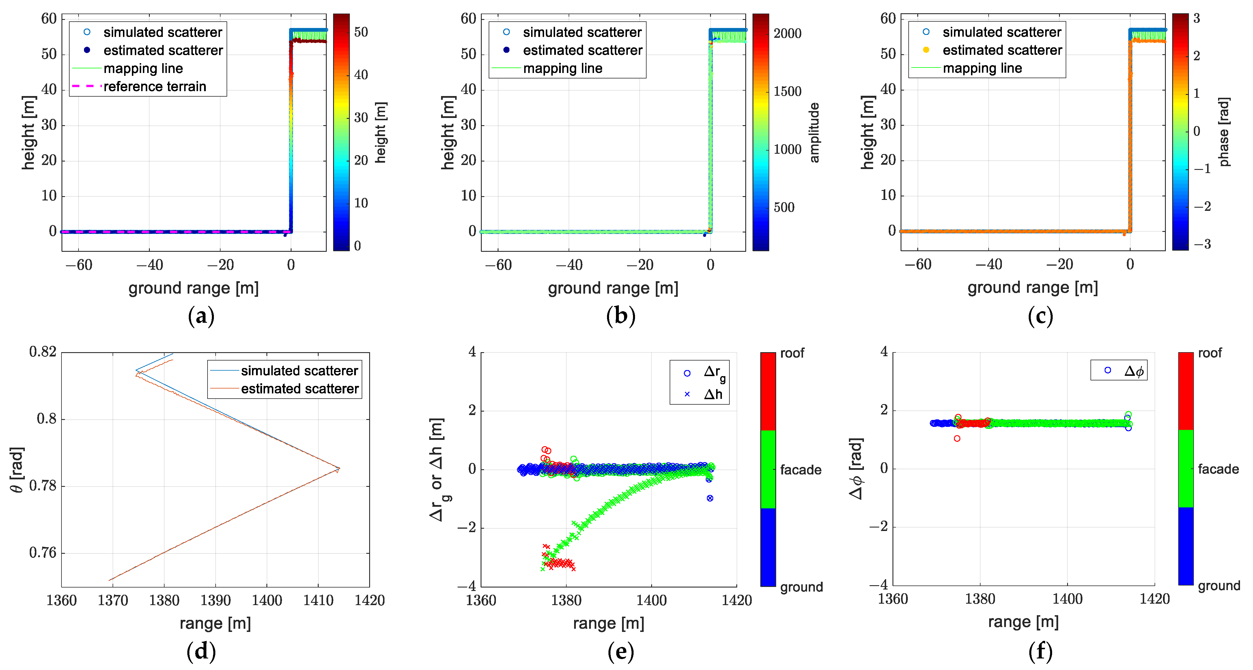
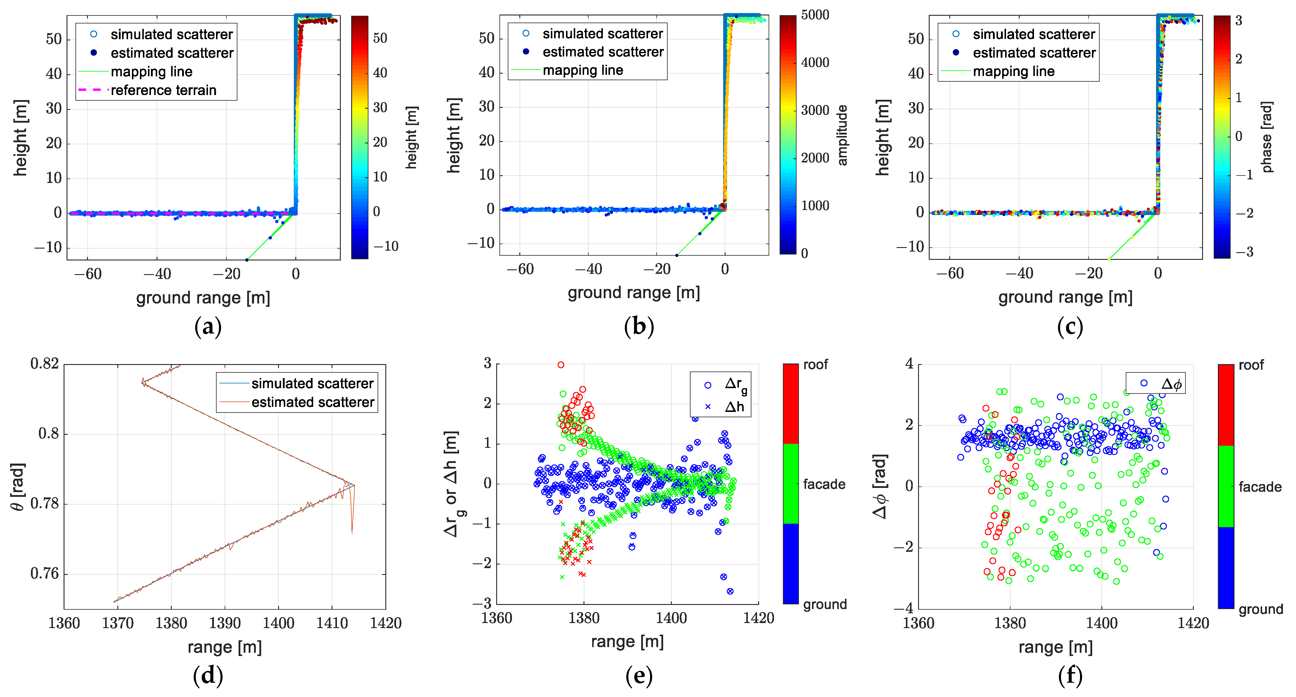
The random phase of scatterers on the ground deteriorates the 3-D reconstruction to a small extent. As shown in Figure 18a, there are some outliers at the façade–ground corner of the building. The off-nadir angle of estimated scatterers is jittering around the simulated off-nadir angle in Figure 18d, which is caused by the random phase of scatterers on the ground. In Figure 18e,f, the error distribution has the same trend as Figure 10e,f. Using the transformation derived in Section 2.4, the positions of scatterers are modified to be close to the simulated scatterers as shown in Figure 19a. The ground range error and height error are around 0 m as shown in Figure 19e. In Figure 19c, the phase of scatterers on the façade and roof are both flat. The phase error between estimated scatterers and simulated scatterers is nearly constant as shown in Figure 19f. Although the error has a wider range as shown in Figure 19e,d compared to Figure 16e,f, we still believe that the conversion method is effective because the ground range error and height error are nearly unbiased and the sample mean of phase error is nearly constant as shown in Table 4.
Although the reconstruction is not perfect like Figure 16, the effectivity of the transformation between model 1 and model 5 in a complex scenario can still be verified.

3.2. Experiments on Measured Data

In this subsection, models 1, 4, 5 and 6 are used to process the measured data. The transformation between model 1 and model 5 and the transformation between model 4 and model 6 are performed in experiments. Two local regions in the illuminated scene are selected to conduct two experiments. In experiment 1, a tower crane with clear structure is chosen as an experimental target to analyze the 3-D reconstruction under different models. In experiment 2, a region with two buildings and the ground between them is selected as an experimental target. The reference terrain is 0 m ground plane.

3.2.1. Measured Dataset

The experiments and discussions are based on the airborne Array-InSAR system by Aerospace Information Research Institute, Chinese Academy of Sciences (AIRCAS) [17]. The system is a Ku-band high-resolution Array-InSAR and data was acquired in Yuncheng City, Shanxi province, China. More details about the system parameters are listed in Table 5.
There are eight channels corresponding to eight antennas in total. The image size of a single channel SAR image is 3100 × 1220 pixels in the azimuth and range directions as shown in Figure 20b.
In experiment 1, a region of 881 × 471 pixels is chosen as the inversion area, as shown in Figure 20c. The tower crane in this region is our experimental target used to visually compare the reconstruction of each model in three dimensions. Due to the overlap between the tower crane and the façade of the building, the structure of the tower crane in Figure 20c cannot be clearly seen. After tomographic processing, the tower crane will be clearly visible. In Table 6, the parameters of this region are listed. Considering the complexity of the scene, in order to avoid the ambiguity of reflectivity function in the third dimension, different off-nadir angle limitations are adopted at different ranges.
Referring to Equation ( 16 ), the length L of the effective integral interval under the planar wavefront models is about 27.19 m and 27.96 m at the near and far ends of the illuminated scene, respectively. Referring to Equation ( 15 ), the maximum length L max of the effective integral interval under the planar wavefront models is 38.46 m and 39.54 m at the near and far ends of the illuminated scene, respectively. The height of the scene is about 80 m. The extension in the elevation direction must be greater than the height of the scene. Therefore, the lengths L and L max are smaller than the length of the extension of the illuminated scene.
In experiment 2, a region of 601 × 301 pixels is selected as the experimental target, as shown in Figure 21c. This region contains parts of two buildings and the ground between them. The continuous ground and façade provide a good experimental scenario for comparing the reconstruction of each model and verifying the validity of the model transformation we proposed. Table 7 summarizes the parameters of the selected region in experiment 2.
Referring to Equation ( 16 ), the length L of the effective integral interval under the planar wavefront models is about 27.96 m and 28.44 m at the near and far ends of the illuminated scene, respectively. Referring to Equation ( 15 ), the maximum length L max of the effective integral interval under the planar wavefront models is 39.54 m and 40.21 m at the near and far ends of the illuminated scene, respectively. The height of the scene is about 60 m. The extension in the elevation direction must be greater than the height of the scene. Therefore, the lengths L and L max are smaller than the length of the extension of the illuminated scene.

3.2.2. Evaluation Methods

Unfortunately, we do not have the ground truth data for this area. Therefore, the absolute accuracy of each model’s reconstruction cannot be evaluated. From Section 3.1, the accuracy of model 5 is verified on simulated data. Model 5 is a spherical wavefront model with the exact form of the slant range. We use the experiments on the measured data to verify the relative relationship between the reconstruction of each model and reconstruction of model 5.
In experiment 1, the relative relationship between tower cranes reconstructed under different models is shown in three dimensions. Moreover, scatterers in a small area as shown in Figure 22b are selected to quantitatively analyze the relationship between the reconstruction of each model.
In experiment 2, the difference of the reconstruction of each model is demonstrated in 2-D images. The ground range and height error of the estimated scatterer can be shown obviously at each azimuth and range position. In addition, histograms provide the distribution of the error.

3.2.3. Results of Experiment 1

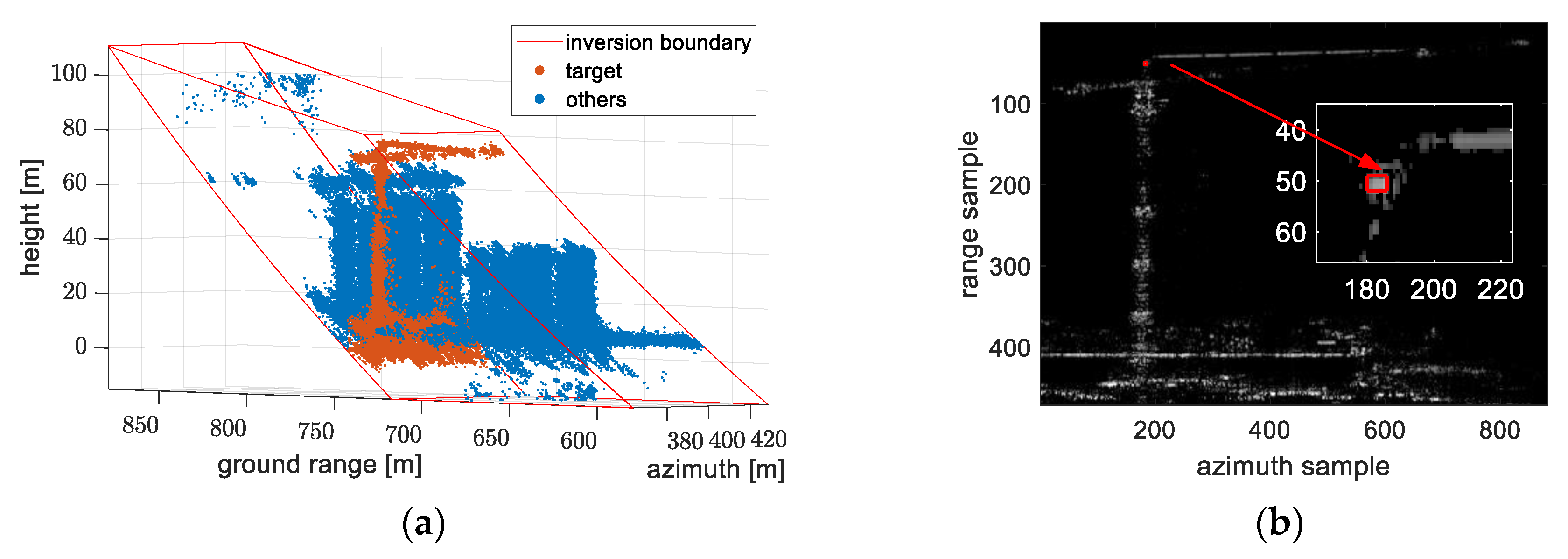
From Section 3.1, we know that model 5 (the exact form of the spherical wavefront model) is accurate, so the measured data is processed under model 5 first to provide a reference. The reconstruction result is shown in Figure 22a. The buildings and the tower crane are clearly visible. The tower crane is shown in orange, and buildings are shown in blue. To give a clearer comparison, we extract the tower crane out of the point cloud of the scene by filtering the ground range of estimated scatterers. Then, we project the tower crane to a 2-D image with the value representing the reflectivity of scatterers, as shown in Figure 22b.
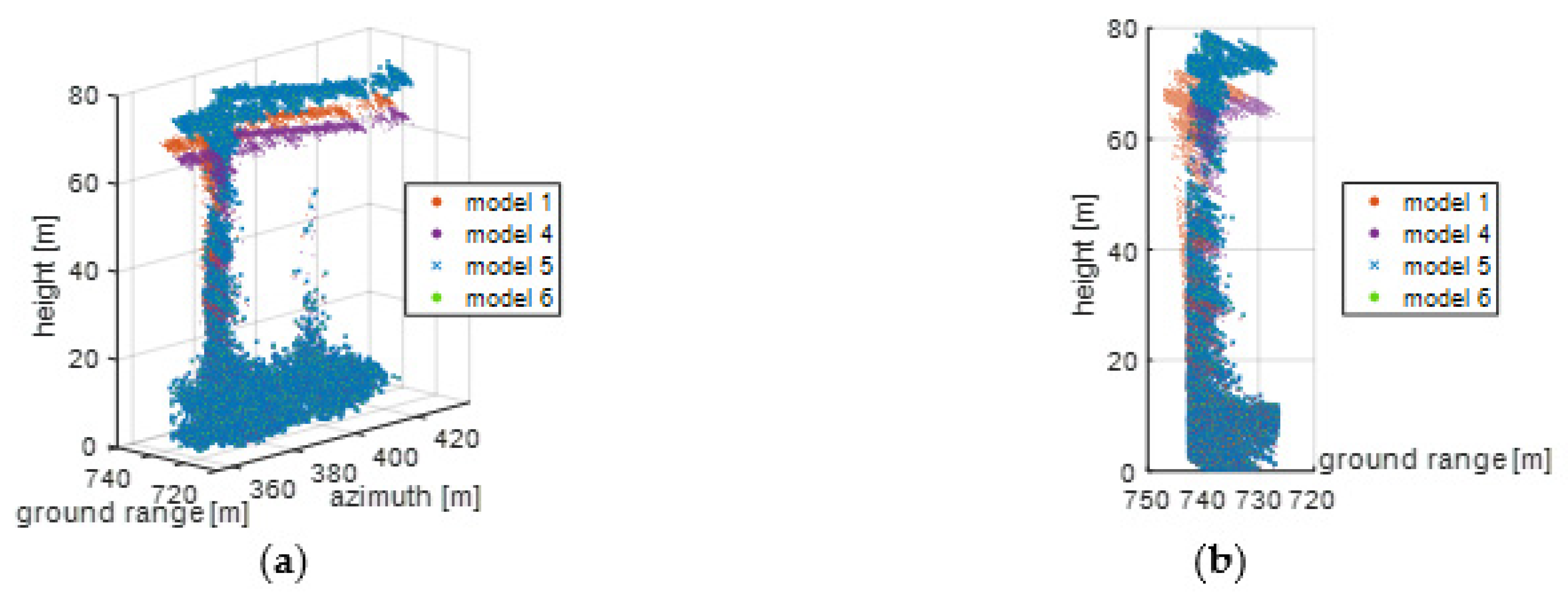
Compared to experiments using simulated data, we do not have ground truth for targets on the ground in experiments using measured data. For this reason, the MAE and RMSE of the positions of estimated scatterers could not be calculated. Firstly, we compare reconstruction results of different models visually. Then, we choose estimated scatterers from the same area in 2-D SAR images under different models to do the quantitative analysis. In Figure 23a,b, the reconstructed tower crane under model 5 (the exact form of the spherical wavefront model) and model 6 (the approximate form of the spherical wavefront model) are similar; the reconstructed tower crane under model 1 (the exact form of the planar wavefront model) deviates from the reconstructed tower crane under model 5 in the direction of line of sight away from the antenna, and the reconstructed tower crane under model 4 (the third approximate form of the planar wavefront model) deviates from the reconstructed tower crane under model 5 in the direction normal to the direction of the baseline. In Figure 23c, the reconstructed tower crane under the transformed model 1 is similar to the reconstructed tower crane under model 5. In Figure 23c, the reconstructed tower crane under the transformed model 4 is similar to the reconstructed tower crane under model 5.
We slice out 7 × 4 pixels in azimuth and range directions as shown in the red frame in Figure 22b to calculate the mean and the standard deviation of the ground range and the height of estimated scatterers in these pixels, and the results are collected in Table 8. The tower crane reconstructed under model 1 is 6.3 m lower than the one under model 5, and the tower crane reconstructed under model 4 is 8.9 m lower than the one under model 5.

3.2.4. Results of Experiment 2

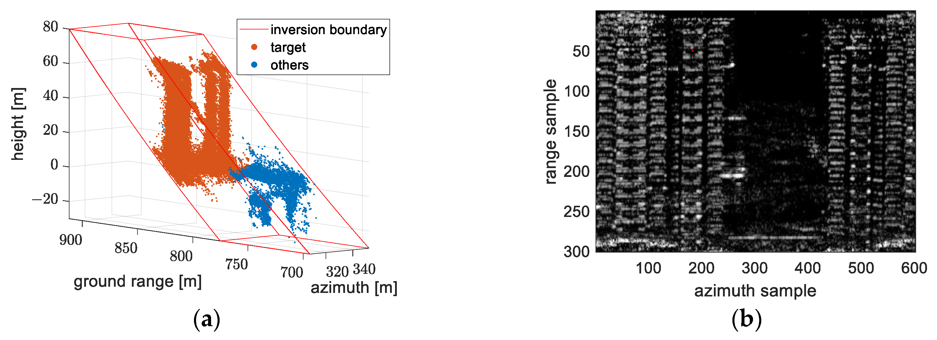
Firstly, the scene is reconstructed using model 5 as shown in Figure 24a. The reconstruction has been filtered to some extent. There are still some outliers caused by multiple scattering in the near end of the scene in the ground range direction. These outliers are not our experimental target. We extract the target by selecting scatterers that appear in a specific range of ground range, and the extracted result is projected in a 2-D image as shown in Figure 24b.
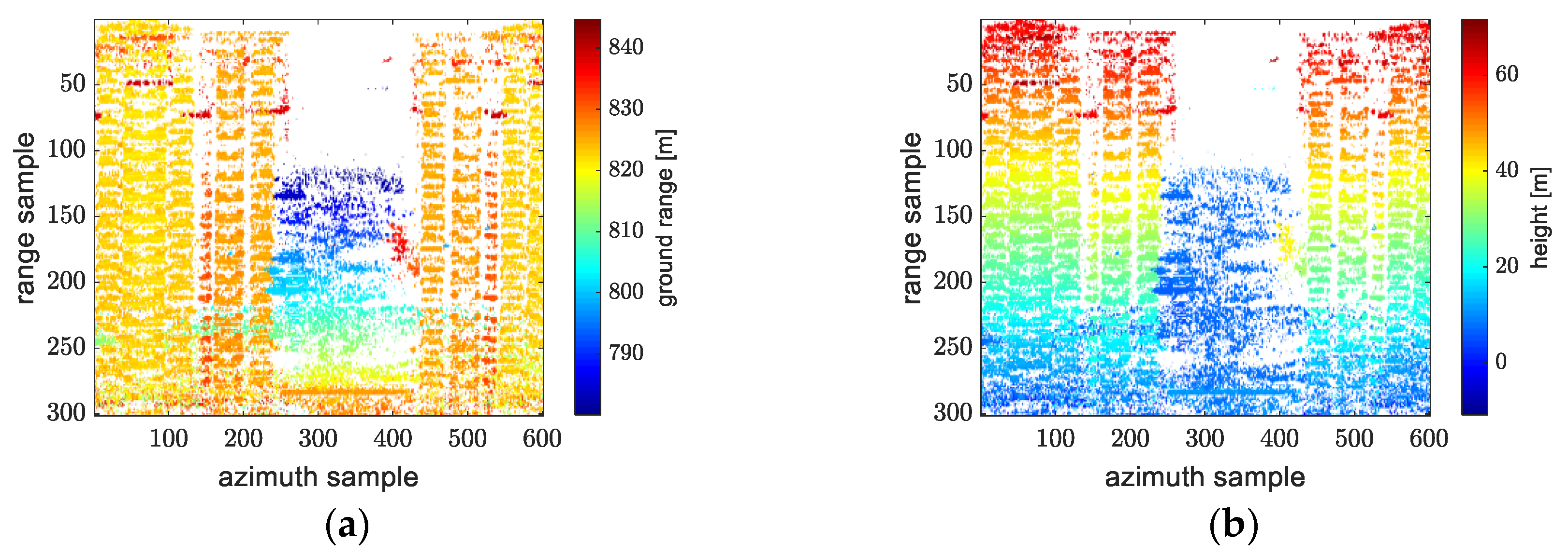
In order to see the ground range and height of the scatterer in each pixel, the 2-D image is colored to refer to ground range and height as shown in Figure 25. White color means that the scatterers in this pixel are filtered out. When there is more than one scatterer in the pixel, the highest scatterer remained. In Figure 25a, pixels in façades at the same azimuth position are in the same color, which means that scatterers in these pixels have the same ground range. In Figure 25b, pixels in an area between two facades are in the same color, which means that scatterers in these pixels have the same height. This is consistent with the fact that the façade is vertical and the ground is horizontal.
To visually compare the difference of the reconstruction obtained by each model, we color the 2-D image refer to the ground range and height error between model 5 and other models. The formulas of the ground range and height error are
Δ r g = r g ( i ) r g ( 5 ) ,   i = 1 , 4   and   6
Δ h = h ( i ) h ( 5 ) ,   i = 1 , 4   and   6
For the transformed models, the formulas are
Δ r g = r g ( i ) r g ( 5 ) ,   i = 1   and   4
Δ h = h ( i ) h ( 5 ) ,   i = 1   and   4
In Figure 26, we can see that the ground range of most scatterers reconstructed using model 1 is greater than for ones reconstructed using model 5, and the height of most scatterers reconstructed using model 1 is less than for ones reconstructed using model 5. This is consistent with the experimental results on simulated data. After using the transformation between model 1 and model 5, there is no difference between reconstructions of transformed model 1 and model 5, ignoring a few pixels as shown in Figure 27. In Figure 27c, the histogram of ground range error and the histogram of height error are overlapping.
To make it easier to understand the phenomenon of the ground range and height error between model 4 and model 5, we compare model 6 and model 5 first. In Figure 28, we can see that there is no difference between reconstructions of model 6 and model 5, ignoring a few pixels, which means that the approximation of the slant range in model 6 does not affect the reconstruction. In Figure 28c, the histogram of ground range error and the histogram of height error are overlapping. Therefore, we can regard the transformation between model 4 and model 6 as the transformation between model 4 and model 5.
If we use the experience obtained from the experiments on simulated data, the ground range error between model 4 and model 5 will be about 0 m. But in this experiment, the error is approximately in the range of ( 1   m , 1   m ) , as shown in Figure 29c. The reason is that the baseline incline angles are not all 0° and are even not equal, as shown in Table 5. For the transformation between model 4 and model 6, the assumption of collinear antennas is not strictly satisfied. Therefore, the scatterers reconstructed under model 4 do not strictly move away from the ones reconstructed under model 5 along the direction normal to the baseline. Since the baseline is close to the horizontal distribution, the height error between model 4 and model 5 is more obvious. After using the transformation between model 4 and model 6, the significant height error is compensated to the level of the ground range error, as shown in Figure 30.

4. Discussion

Models 1, 2, 3 and 4 are based on a planar wavefront geometry. Scatterers estimated with model 1 will move away from their correct positions along the direction of the LOS when they are not on the reference LOS. The farther away the scatterer is from the reference LOS, the farther away it is from its correct position. The reconstruction of model 2 is basically the same as that of model 1, despite some approximation of the slant range. After further approximating, the reconstruction of model 3 shows new characteristics. Scatterers estimated with model 3 move away from their correct positions along the direction normal to the baseline. Omitting a second-order phase about elevation, the reconstruction of model 4 is the same as model 3 in terms of the positions of scatterers. Models 5 and 6 proposed by us are based on a spherical wavefront geometry. The reconstructions of these two models are very accurate. The transformation between model 1 and model 5 and the transformation between model 4 and model 6 are derived and proved. These transformations provide support for the transplantation of tomography algorithms based on the traditional model to the low-altitude airborne case and the conversion of reconstructions obtained by the traditional model to ones under the spherical wavefront models we proposed.
The computation time of each model is nearly the same. The computation time is mainly dependent on tomography algorithms. These models are adopted in the pixel-by-pixel processing framework of TomoSAR imaging. This framework is based on an assumption that the 2-D SAR images are well coregistered. However, in low-altitude airborne cases, image coregistration becomes a new challenge. The discretization of models is performed with the assumption that the reflectivity function of the illuminated scene is sparse in the third dimension. When some distributed targets appear in the scene, the sparsity assumption will no longer be satisfied.

5. Conclusions

In this paper, the power of TomoSAR in building modeling is demonstrated. With the improvement of data quality and the expansion of the variety of SAR platforms, more accurate TomoSAR imaging models are urgently needed.
The conventional TomoSAR imaging models based on planar wavefront geometry can no longer provide a satisfactory image reconstruction in the low-altitude airborne case. For a more accurate reconstruction of the illuminated scene, TomoSAR imaging models based on spherical wavefront geometry are proposed. The 3-D reconstructions of illuminated scenes using these models were compared and the effectiveness of transformation methods were proved through experiments on simulated data and real data.

Author Contributions

Conceptualization, Q.Y., Z.J. and X.Q.; methodology, Q.Y. and Z.J.; software, Q.Y., Z.J. and X.Q.; validation, Q.Y.; formal analysis, Q.Y., Z.J. and X.Q.; investigation, Q.Y.; resources, Z.J., X.Q. and C.D.; data curation, Z.J. and B.W.; writing—original draft preparation, Q.Y. and Z.J.; writing—review and editing, Q.Y. and Z.J.; visualization, Q.Y. and Z.J.; supervision, Z.J., X.Q., B.W. and C.D.; project administration, Z.J., X.Q. and C.D.; funding acquisition, Z.J., X.Q. and C.D. All authors have read and agreed to the published version of the manuscript.

Funding

This research was funded by the National Natural Science Foundation of China (No. 62101535, No. 61991420 and No. 61991421).

Data Availability Statement

The experimental data comes from the “SARMV3D-1.0: Synthetic Aperture Radar Microwave Vision 3D Imaging Dataset” which is available from the website of the Journal of Radars (https://radars.ac.cn/web/data/getData?dataType=SARMV3D, accessed on 1 February 2022).

Acknowledgments

The authors thank the staff of the National Key Laboratory of Microwave Imaging Technology, Institute of Electronics, Chinese Academy of Sciences, for their hard work in the airborne array TomoSAR system design and the acquisition of real data.

Conflicts of Interest

The authors declare no conflict of interest.

References

  1. Moreira, A.; Prats-Iraola, P.; Younis, M.; Krieger, G.; Hajnsek, I.; Papathanassiou, K.P. A Tutorial on Synthetic Aperture Radar. IEEE Geosci. Remote Sens. Mag. 2013, 1, 6–43. [Google Scholar] [CrossRef] [Green Version]
  2. Massonnet, D.; Rabaute, T. Radar interferometry: Limits and potential. IEEE Trans. Geosci. Remote Sens. 1993, 31, 455–464. [Google Scholar] [CrossRef]
  3. Ferretti, A.; Prati, C.; Rocca, F. Permanent scatterers in SAR interferometry. IEEE Trans. Geosci. Remote Sens. 2001, 39, 8–20. [Google Scholar] [CrossRef]
  4. Pasquali, P.; Prati, C.; Rocca, F.; Seymour, H. A 3-D SAR experiment with EMSL data. In Proceedings of the 1995 International Geoscience and Remote Sensing Symposium (IGARSS 95), Florence, Italy, 10–14 July 1995; pp. 784–786. [Google Scholar]
  5. Knaell, K.K. Radar tomography for the generation of three-dimensional images. IEE Proc. -Radar. Sonar Navig. 1995, 142, 54–60. [Google Scholar] [CrossRef] [Green Version]
  6. Reale, D.; Pauciullo, A.; Fornaro, G.; Maio, A.D. A scatterers detection scheme in SAR Tomography for reconstruction and monitoring of individual buildings. In Proceedings of the 2011 Joint Urban Remote Sensing Event, 11–13 April 2011; pp. 249–252. [Google Scholar]
  7. Wu, X.; Jezek, K.C.; Rodriguez, E.; Gogineni, S.; Rodriguez-Morales, F.; Freeman, A. Ice Sheet Bed Mapping with Airborne SAR Tomography. IEEE Trans. Geosci. Remote Sens. 2011, 49, 3791–3802. [Google Scholar] [CrossRef]
  8. Quegan, S.; Le Toan, T.; Chave, J.; Dall, J.; Exbrayat, J.-F.; Minh, D.H.T.; Lomas, M.; D’Alessandro, M.M.; Paillou, P.; Papathanassiou, K.; et al. The European Space Agency BIOMASS mission: Measuring forest above-ground biomass from space. Remote Sens. Environ. 2019, 227, 44–60. [Google Scholar] [CrossRef] [Green Version]
  9. Nannini, M.; Scheiber, R.; Horn, R.; Moreira, A. First 3-D Reconstructions of Targets Hidden Beneath Foliage by Means of Polarimetric SAR Tomography. IEEE Geosci. Remote Sens. Lett. 2012, 9, 60–64. [Google Scholar] [CrossRef] [Green Version]
  10. Reigber, A.; Moreira, A. First demonstration of airborne SAR tomography using multibaseline L-band data. IEEE Trans. Geosci. Remote Sens. 2000, 38, 2142–2152. [Google Scholar] [CrossRef]
  11. Yu, Y.; d’Alessandro, M.M.; Tebaldini, S.; Liao, M. Signal Processing Options for High Resolution SAR Tomography of Natural Scenarios. Remote Sens. 2020, 12, 1638. [Google Scholar] [CrossRef]
  12. Ren, Y.; Xiao, A.; Hu, F.; Xu, F.; Qiu, X.; Ding, C.; Jin, Y.-Q. Coprime Sensing for Airborne Array Interferometric SAR Tomography. IEEE Trans. Geosci. Remote Sens. 2022, 60, 1–15. [Google Scholar] [CrossRef]
  13. Rambour, C.; Denis, L.; Tupin, F.; Oriot, H.M. Introducing Spatial Regularization in SAR Tomography Reconstruction. IEEE Trans. Geosci. Remote Sens. 2019, 57, 8600–8617. [Google Scholar] [CrossRef] [Green Version]
  14. Zhu, X.X.; Bamler, R. Very High Resolution Spaceborne SAR Tomography in Urban Environment. IEEE Trans. Geosci. Remote Sens. 2010, 48, 4296–4308. [Google Scholar] [CrossRef] [Green Version]
  15. Fornaro, G.; Lombardini, F.; Serafino, F. Three-dimensional multipass SAR focusing: Experiments with long-term spaceborne data. IEEE Trans. Geosci. Remote Sens. 2005, 43, 702–714. [Google Scholar] [CrossRef]
  16. Rambour, C.; Budillon, A.; Johnsy, A.C.; Denis, L.; Tupin, F.; Schirinzi, G. From Interferometric to Tomographic SAR: A Review of Synthetic Aperture Radar Tomography-Processing Techniques for Scatterer Unmixing in Urban Areas. IEEE Geosci. Remote Sens. Mag. 2020, 8, 6–29. [Google Scholar] [CrossRef]
  17. Ding, C.; Qiu, X.; Xu, F.; Liang, X.; Jiao, Z.; Zhang, F. Synthetic Aperture Radar Three-dimensional Imaging—From TomoSAR and Array InSAR to Microwave Vision. J. Radars 2019, 8, 693–709. [Google Scholar]
  18. Fornaro, G.; Serafino, F.; Soldovieri, F. Three-dimensional focusing with multipass SAR data. IEEE Trans. Geosci. Remote Sens. 2003, 41, 507–517. [Google Scholar] [CrossRef]
  19. Zhu, X.X.; Bamler, R. Tomographic SAR Inversion by L1-Norm Regularization—The Compressive Sensing Approach. IEEE Trans. Geosci. Remote Sens. 2010, 48, 3839–3846. [Google Scholar] [CrossRef]
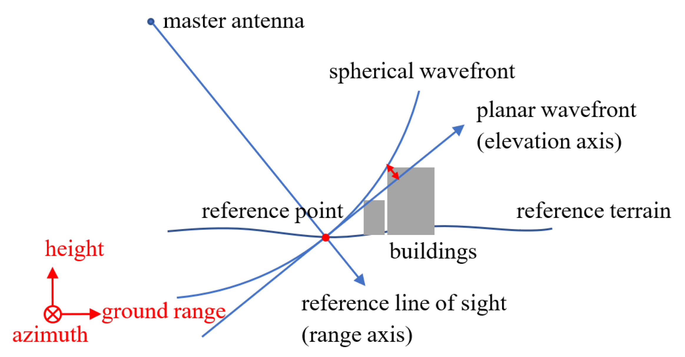
Figure 1. The difference between a planar wavefront and a spherical wavefront in TomoSAR imaging geometry.
Remotesensing 14 05452 g001
Figure 2. TomoSAR imaging geometry based on a planar wavefront.
Remotesensing 14 05452 g002
Figure 3. The effective integral interval under the planar wavefront model: (a) the maximum length of the effective integral interval, (b) the common length of the effective integral interval.
Remotesensing 14 05452 g003
Figure 4. TomoSAR imaging geometry based on a spherical wavefront geometry.
Remotesensing 14 05452 g004
Figure 5. The difference of the range from antennas to the scatterer along off-nadir angle under model 1 and model 5 using the parameters of the simulation experiment mentioned in Section 3.1.
Remotesensing 14 05452 g005
Figure 6. The frames and geometry of TomoSAR imaging model. The ground frame is in black. The radar frame of the planar wavefront model is in blue. The radar frame of the spherical wavefront model is in green. And the baseline frame is in red.
Remotesensing 14 05452 g006
Figure 7. (a) Configuration of the antenna array; (b) structure of the simulated scene in ground frame.
Remotesensing 14 05452 g007
Figure 8. The simulated scenario in experiment 1: (a) the amplitude of simulated scatterers, (b) the phase of simulated scatterers, (c) the 2-D SAR image from master antenna.
Remotesensing 14 05452 g008
Figure 9. The simulated scenario in experiment 2: (a) the amplitude of simulated scatterers, (b) the phase of simulated scatterers, (c) the 2-D SAR image from master antenna.
Remotesensing 14 05452 g009
Figure 10. The reconstruction obtained using model 1 (the exact form of the planar wavefront model): (a) reconstruction with colors denoted as height, (b) reconstruction with colors denoted as amplitude, (c) reconstruction with colors denoted as phase, (d) the off-nadir angle of the reconstruction, (e) the error of the ground range and height, (f) the error of the phase.
Remotesensing 14 05452 g010
Figure 11. The reconstruction obtained using model 2 (the first approximate form of the planar wavefront model): (a) reconstruction with colors denoted as height, (b) reconstruction with colors denoted as amplitude, (c) reconstruction with colors denoted as phase, (d) the off-nadir angle of the reconstruction, (e) the error of the ground range and height, (f) the error of the phase.
Remotesensing 14 05452 g011
Figure 12. The reconstruction obtained using model 3 (the second approximate form of the planar wavefront model): (a) reconstruction with colors denoted as height, (b) reconstruction with colors denoted as amplitude, (c) reconstruction with colors denoted as phase, (d) the off-nadir angle of the reconstruction, (e) the error of the ground range and height, (f) the error of the phase.
Remotesensing 14 05452 g012
Figure 13. The reconstruction obtained using model 4 (the third approximate form of the planar wavefront model): (a) reconstruction with colors denoted as height, (b) reconstruction with colors denoted as amplitude, (c) reconstruction with colors denoted as phase, (d) the off-nadir angle of the reconstruction, (e) the error of the ground range and height, (f) the error of the phase.
Remotesensing 14 05452 g013
Figure 14. The reconstruction obtained using model 5 (the exact form of the spherical wavefront model): (a) reconstruction with colors denoted as height, (b) reconstruction with colors denoted as amplitude, (c) reconstruction with colors denoted as phase, (d) the off-nadir angle of the reconstruction, (e) the error of the ground range and height, (f) the error of the phase.
Remotesensing 14 05452 g014
Figure 15. The reconstruction obtained using model 6 (the approximate form of the spherical wavefront model): (a) reconstruction with colors denoted as height, (b) reconstruction with colors denoted as amplitude, (c) reconstruction with colors denoted as phase, (d) the off-nadir angle of the reconstruction, (e) the error of the ground range and height, (f) the error of the phase.
Remotesensing 14 05452 g015
Figure 16. The reconstruction obtained under model 1 (the exact form of the planar wavefront model) after transformation: (a) reconstruction with colors denoted as height, (b) reconstruction with colors denoted as amplitude, (c) reconstruction with colors denoted as phase, (d) the off-nadir angle of the reconstruction, (e) the error of the ground range and height, (f) the error of the phase.
Remotesensing 14 05452 g016
Figure 17. The reconstruction obtained under model 4 (the approximate form of the planar wavefront model) after transformation: (a) reconstruction with colors denoted as height, (b) reconstruction with colors denoted as amplitude, (c) reconstruction with colors denoted as phase, (d) the off-nadir angle of the reconstruction, (e) the error of the ground range and height, (f) the error of the phase.
Remotesensing 14 05452 g017aRemotesensing 14 05452 g017b
Figure 18. The reconstruction obtained under model 1 (the exact form of the planar wavefront model) in experiment 2: (a) reconstruction with colors denoted as height, (b) reconstruction with colors denoted as amplitude, (c) reconstruction with colors denoted as phase, (d) the off-nadir angle of the reconstruction, (e) the error of the ground range and height, (f) the error of the phase.
Remotesensing 14 05452 g018
Figure 19. The reconstruction obtained under model 1 (the exact form of the planar wavefront model) after transformation in experiment 2: (a) reconstruction with colors denoted as height, (b) reconstruction with colors denoted as amplitude, (c) reconstruction with colors denoted as phase, (d) the off-nadir angle of the reconstruction, (e) the error of the ground range and height, (f) the error of the phase.
Remotesensing 14 05452 g019aRemotesensing 14 05452 g019b
Figure 20. The selected region in experiment 1: (a) the configuration of the antenna array. The 2-D SAR image of the measured data: (b) the whole scene and (c) the inversion area in the red frame in (b).
Remotesensing 14 05452 g020
Figure 21. The selected region in experiment 2: (a) the configuration of the antenna array. The 2-D SAR image of the measured data: (b) the whole scene and (c) the inversion area in the green frame in (b).
Remotesensing 14 05452 g021
Figure 22. The tower crane extracted from the selected region in experiment 1: (a) 3-D point cloud containing the tower crane and buildings; (b) 2-D SAR image corresponding to the tower crane. The red frame in (b) is used for the quantitative analysis of the reconstructions under different models.
Remotesensing 14 05452 g022
Figure 23. The reconstructed tower crane (a) under model 1 (the exact form of the planar wavefront model), 4 (the third approximate form of the planar wavefront model), 5 (the exact form of the spherical wavefront model) and 6 (the approximate form of the spherical wavefront model); (b) in the ground range–height plane; (c) under model 1, transformed model 1 and model 5; (d) under model 4, transformed model 4 and model 5.
Remotesensing 14 05452 g023aRemotesensing 14 05452 g023b
Figure 24. The target extracted from the selected region in experiment 2: (a) 3-D point cloud containing the target and others; (b) 2-D SAR image corresponding to the target.
Remotesensing 14 05452 g024
Figure 25. The target obtained by model 5 (the exact form of the spherical wavefront model) and shown in (a) 3-D point cloud and (b) 2-D SAR image.
Remotesensing 14 05452 g025
Figure 26. The ground range and height error between model 1 and model 5: (a) the ground range error; (b) the height error; (c) a histogram of the ground range and height error.
Remotesensing 14 05452 g026
Figure 27. The ground range and height error between transformed model 1 and model 5: (a) the ground range error; (b) the height error; (c) a histogram of ground range and height error.
Remotesensing 14 05452 g027
Figure 28. The ground range and height error between model 6 and model 5: (a) the ground range error; (b) the height error; (c) a histogram of the ground range and height error.
Remotesensing 14 05452 g028
Figure 29. The ground range and height error between model 4 and model 5: (a) the ground range error; (b) the height error; (c) a histogram of the ground range and height error.
Remotesensing 14 05452 g029
Figure 30. The ground range and height error between transformed model 4 and model 5: (a) the ground range error; (b) the height error; (c) a histogram of the ground range and height error.
Remotesensing 14 05452 g030
Table 1. Details of models.
GeometricPixel FormulaRange FormulaGeodetic Transform
model 1planar wavefront(2)(3)(13)
model 2planar wavefront(2)(10)(13)
model 3planar wavefront(2)(11)(13)
model 4planar wavefront(2)(12)(13)
model 5spherical wavefront(17)(18)(22)
model 6spherical wavefront(17)(21)(22)
Table 2. Parameters of simulated data.
ParameterSymbolValue
Wavelength λ 0.02 m
Range resolution ρ r 0.25 m
Azimuth resolution ρ a 0.2083 m
Flight height h 0 1000 m
Channel number M 8
Baseline length b m 0 m, 0.141 m, 0.283 m, 0.424 m, 0.566 m, 0.707 m, 0.848 m, 0.990 m
Baseline incline angle α m 0°, 0°, 0°, 0°, 0°, 0°, 0°, 0°
Range r 0 1369.2 m~1414.2 m
Minimum off-nadir angle θ min 43.0846°
Maximum off-nadir angle θ max 46.9648°
Table 3. The quantitative analysis of inversion results using simulated data in experiment 1.
Ground Range (m)Height (m)Phase (rad)Amplitude
MERMSEMERMSE μ Δ ϕ σ Δ ϕ μ A σ A
Model 1Roof1.8151.822−1.5171.5240.2141.8841055.6184.8
Façade0.5230.750−0.5800.754−0.2111.8431157.1127.0
Ground00.10300.1021.5710.0491130.491.7
Model 4Roof0.1040.218−3.1393.1441.5500.1081051.6211.8
Façade−0.0200.094−1.0991.4721.5720.0341157.6136.0
Ground0.0070.1040.0070.1031.5650.0241129.991.6
Model 5Roof0.0930.1810.0980.1931.5530.0901055.8184.5
Façade−0.0400.100−0.0410.1031.5760.0331157.1126.9
Ground00.10400.1021.5660.0241130.491.7
Model 6Roof0.0930.1810.0980.1931.5530.0901056.3184.0
Façade−0.0400.100−0.0410.1031.5760.0341157.0126.7
Ground00.10400.1021.5660.0241130.491.7
Transformed
Model 1
Roof0.0930.1810.0980.1931.5530.0901055.6184.8
Façade−0.0400.100−0.0410.1031.5760.0331157.1127.0
Ground00.10400.1021.5660.0241130.491.7
Transformed
Model 4
Roof0.1040.2180.1100.2321.5500.1081051.6211.8
Façade−0.0200.094−0.0200.0971.5720.0341157.6136.0
Ground0.0070.1040.0070.1021.5650.0241129.991.6
Table 4. The quantitative analysis of inversion results using simulated data in experiment 2.
Ground Range (m)Height (m)Phase (rad)Amplitude
MERMSEMERMSE μ Δ ϕ σ Δ ϕ μ A σ A
Model 1Roof1.7421.787−1.5861.630−0.4271.6242562.61551.0
Façade0.5280.752−0.5760.7800.0321.7823629.11510.6
Ground−0.1221.238−0.1221.2331.6070.5221137.41236.5
Transformed
Model 1
Roof0.0240.3740.0250.3991.5180.3272562.61551.0
Façade−0.0360.178−0.0370.1831.5740.0633629.11510.6
Ground−0.1231.2440.1211.2271.5910.3271137.41236.5
Table 5. System parameters of the measured data.
ParameterSymbolValue
Wavelength λ 0.021 m
Range resolution ρ r 0.1499 m
Azimuth resolution ρ a 0.0734 m
Flight height h 0 1073.621 m
Channel number M 8
Baseline length b m 0 m, 0.084 m, 0.170 m, 0.252 m, 0.336 m, 0.420 m, 0.504 m, 0.588 m
Baseline incline angle α m 0°, 0.726°, 0.725°, 0.747°, 0.742°, 0.738°, 0.747°, 0.734°
Table 6. Parameters of the selected region in experiment 1.
ParameterSymbolValue
Range r 0 1233.196 m~1303.647 m
Minimum off-nadir angle at different ranges θ min ( r 0 ) 28.022°~33.378°
Maximum off-nadir angle at different ranges θ max ( r 0 ) 36.448°~42.392°
Table 7. Parameters of the selected region in experiment 2.
ParameterSymbolValue
Range r 0 1303.647 m~1348.616 m
Minimum off-nadir angle at different ranges θ min ( r 0 ) 32.160°~35.081°
Maximum off-nadir angle at different ranges θ max ( r 0 ) 40.342°~42.542°
Table 8. The quantitative analysis of inversion results using measured data.
Ground Range (m)Height (m)
μ σ μ σ
Model 1742.9680.87670.2470.516
Model 4738.4740.78467.6450.488
Model 5738.2690.80676.5930.607
Model 6738.2970.81776.6130.612
Transformed model 1738.2690.80676.5930.607
Transformed model 4738.3580.78276.6590.625
Publisher’s Note: MDPI stays neutral with regard to jurisdictional claims in published maps and institutional affiliations.