Article

Detecting the Greatest Changes in Global Satellite-Based Precipitation Observations

1
Faculty of Natural Resources, University of Tehran, Karaj 31587-77871, Iran
2
Department of Water Resources Engineering, Faculty of Engineering, Lund University, 221 00 Lund, Sweden
3
Centre for Advanced Middle Eastern Studies, Faculty of Social Sciences, Lund University, 221 00 Lund, Sweden
4
Department of Technology and Society, Faculty of Engineering, Lund University, 221 00 Lund, Sweden
5
NASA Goddard Space Flight Center, Code 612, 8800 Greenbelt Road, Greenbelt, MD 20771, USA
*
Author to whom correspondence should be addressed.
Remote Sens. 2022, 14(21), 5433; https://doi.org/10.3390/rs14215433
Submission received: 12 September 2022 / Revised: 20 October 2022 / Accepted: 25 October 2022 / Published: 28 October 2022

Abstract

:
In recent years, the analysis of abrupt and non-abrupt changes in precipitation has received much attention due to the importance of climate change-related issues (e.g., extreme climate events). In this study, we used a novel segmentation algorithm, DBEST (Detecting Breakpoints and Estimating Segments in Trend), to analyze the greatest changes in precipitation using a monthly pixel-based satellite precipitation dataset (TRMM 3B43) at three different scales: (i) global, (ii) continental, and (iii) climate zone, during the 1998–2019 period. We found significant breakpoints, 14.1%, both in the form of abrupt and non-abrupt changes, in the global scale precipitation at the 0.05 significance level. Most of the abrupt changes were observed near the Equator in the Pacific Ocean and Asian continent, relative to the rest of the globe. Most detected breakpoints occurred during the 1998–1999 and 2009–2011 periods on the global scale. The average precipitation change for the detected breakpoint was ±100 mm, with some regions reaching ±3000 mm. For instance, most portions of northern Africa and Asia experienced major changes of approximately +100 mm. In contrast, most of the South Pacific and South Atlantic Ocean experienced changes of −100 mm during the studied period. Our findings indicated that the larger areas of Africa (23.9%), Asia (22.9%), and Australia (15.4%) experienced significant precipitation breakpoints compared to North America (11.6%), South America (9.3%), Europe (8.3%), and Oceania (9.6%). Furthermore, we found that the majority of detected significant breakpoints occurred in the arid (31.6%) and polar (24.1%) climate zones, while the least significant breakpoints were found for snow-covered (11.5%), equatorial (7.5%), and warm temperate (7.7%) climate zones. Positive breakpoints’ temporal coverage in the arid (54.0%) and equatorial (51.9%) climates were more than those in other climates zones. Here, the findings indicated that large areas of Africa and Asia experienced significant changes in precipitation (−250 to +250 mm). Compared to the average state (trend during a specific period), the greatest changes in precipitation were more abrupt and unpredictable, which might impose a severe threat to the ecology, environment, and natural resources.

Graphical Abstract

1. Introduction

Precipitation change analysis is of great importance on different temporal and spatial scales, given the global climate change [1]. Precipitation directly affects society and the environment and varies spatiotemporally from region to region, year to year, and over decades in frequency, amount, intensity, and type, i.e., rain vs. snow [2]. Global assessment of precipitation changes provides insight into Earth’s climatology over land areas, especially populated regions, as well as over water bodies [3]. On regional and global scales, changes in precipitation characteristics are the most relevant aspects of climate change in a warming world. However, there is little consensus on the expected and observed changes in spatiotemporal precipitation patterns [4]. While no significant change in total precipitation has been detected globally [2], a notable increase in precipitation extremes, wet and drought periods, has been observed (e.g., [5,6]), with projected increases in future extremes (e.g., [7,8]).
The spatial pattern of precipitation changes is heterogeneous, with different regions depicting opposing trends at the global scale [4,9]. Changes in precipitation at different temporal and spatial scales include not only continuous or gradual changes, which can be investigated by conventional trend analysis methods (e.g., ordinary linear regression, Mann–Kendall, and Mann–Whitney), but also discontinuous or abrupt changes in precipitation amount [10]. Further, a practical problem in analyzing precipitation time series is that such data are not always homogeneous and include abrupt changes in the mean [11]. Abrupt changes, referred to as breakpoints or inhomogeneities, are periods of discontinuity in the time series caused by sudden changes in the climate, environment, measurement techniques, observation locations, or equipment. It is noteworthy that many breakpoints occur without documentation, while a breakpoint-free precipitation record is less likely to occur. Therefore, before investigating the precipitation variation and trends, the relative homogeneity in abrupt changes in the time series should be assessed [12].
Effective identification of breakpoints in precipitation records is crucial for understanding the changes over a short period as well as detecting the causal relationships between climate and environment [13]. Breakpoint detection can be conducted using online (or sequential) or offline (or retrospective) approaches. A sequential approach is used when it is necessary to detect the changes in real time. The retrospective breakpoint detection approach is commonly used in meteorology and hydrological applications using a classical statistical test to detect slope changes in the precipitation time series [14,15,16].
Several techniques have been used for testing homogeneity concerning breakpoints in precipitation data [11]. The Worsley’s likelihood ratio test [17], cumulative deviations [18], Von Neumann ratio test [18], Pettitt test [19], standard normal homogeneity test, SNHT [20], and clustering approach [21] are the commonly applied techniques in precipitation breakpoint detection studies. Moreover, Vincent [22] introduced a method based on the classical F and Durbin–Watson tests to detect a breakpoint in time series. Seidou and Ouarda [15] proposed a Bayesian change point method to evaluate abrupt changes in hydro-climatic variables.
Due to the large number of available statistical breakpoint detection tests, understanding the sensitivities to changes (e.g., changes in mean, median, or standard deviation of time series) and characteristics of alternative tests is crucial to arrive at a valid interpretation of the precipitation time series analysis. The classical statistical abrupt change detection tests are sensitive to specific features such as time series mean and deviation. Thus, a statistical test that is only sensitive to a particular type of homogeneity or abrupt change might not provide a comprehensive detection of abrupt changes [23,24]. For instance, the SNHT usually has higher sensitivity to breaks near the start and end portions of the time series, while the Pettitt test is suitable for detecting breaks near the middle part of the time series [19,20,23]. Recently, Jamali et al. [25] developed a user-friendly algorithm for time series analysis, with two main application domains: (i) detecting and characterizing trend changes and (ii) generalizing trends for main features. The method in the present study, Detecting Breakpoints and Estimating Segments in Trend (DBEST), uses a novel segmentation algorithm that simplifies the trend into linear segments with one of three user-defined parameters: the m largest changes, a generalization-threshold parameter, δ, or a threshold, β, for the magnitude of changes of interest for detection. DBEST is based on Bayesian Information Criterion (BIM) [26] and statistical tests [27] to detect statistically significant breakpoints. DBEST outputs are change type (non-abrupt or abrupt), simplified trend, and estimates for the change characteristics (magnitude and timing). DBEST is a flexible, fast, and accurate tool that is applicable to global change studies using the time series of remotely sensed datasets [25].
While there are numerous studies on breakpoint detection using standard statistical tests (e.g., Von Neumann ratio test, SNHT, and Pettitt test) in precipitation data at local and regional scales [4,28,29], there is no comprehensive study, to the best of our knowledge, on the detection of both abrupt and non-abrupt changes at the global scale. This study focused on analyzing abrupt and non-abrupt changes at a quasi-global scale, representing different climatological characteristics of precipitation of the world’s wet and dry regions [4]. We applied the DBEST algorithm to detect significant breakpoints (statistically), investigate their type (non-abrupt or abrupt), and estimate their characteristics (timing and magnitude) in a quasi-global monthly satellite-based precipitation dataset over the 1998–2019 period. While evaluating abrupt and non-abrupt precipitation changes at a quasi-global scale, we investigated continental changes and their associations depending on climate zones.

2. Materials and Methods

2.1. Data Sources

We used the Tropical Rainfall Measuring Mission (TRMM) Multi-satellite Precipitation Analysis (TMPA) product, in which the National Aeronautics and Space Administration (NASA) estimates quasi-global precipitation. TRMM TMPA data are produced based on the constellation of passive microwave and infrared sensors onboard multiple partners’ satellites [30,31]. The core observatory, TRMM, was a collaboration between the Japan Aerospace Exploration Agency (JAXA) and NASA; it was launched in November 1997 and ended its mission in April 2015. However, the TMPA algorithm continued producing precipitation data using partner satellites through to the end of 2019. TMPA Version 7 provides products at 3-hourly (3B42), daily (3B42-derived), and monthly (3B43) temporal resolutions, in the latitude band 50°N-S at 0.25° × 0.25° spatial resolution [30,32] for the period 1998–2019. Monthly TMPA-3B43 v7.0 is one of the most widely used products for climate and research purposes [30,33]. It is noteworthy that the transition from TMPA to Integrated Multi-satellite Retrievals for the Global Precipitation Measurement (GPM) mission (IMERG) began in 2015, and the IMERG data are now available for the 2000–present period. While IMERG provides a more detailed precipitation dataset (temporally and spatially), a thorough validation of its products continues to be conducted for use in global-scale analyses. A detailed description of the TMPA and IMERG algorithms and input data can be found in Huffman et al. [34], as well as Huffman et al. [30], Huffman and Bolvin [35], and Huffman [36].
The TRMM products have been used extensively in many regions around the world. Their spatiotemporal performance has been thoroughly validated by ground-based measurements all over the globe [37], such as in the United States [38,39,40,41,42], India [43,44,45], China [46,47], Iran [48,49,50], the Philippines [51], Eastern Africa [52], and Malaysia [53], to mention a few. In this study, we used the TMPA 3B43 research product at a monthly time scale from January 1998 to December 2019. The TMPA 3B43 product used in this study incorporates bias-corrected surface precipitation gauge analyses. Thus, it takes advantage of gauge information, where available, and the multi-satellite scheme everywhere.

2.2. Methods

2.2.1. Breakpoint Detection

The DBEST algorithm has two main application domains: trend generalization and change detection. We used the change detection method, which a novel segmentation algorithm that simplifies the trend into linear segments using the m largest changes or a threshold, β, for detection’s magnitude of change of interest (Table 1).
Here, we briefly describe the DBEST’s change detection workflow along with the threshold values used in this study. DBEST starts with testing the existence of significant discontinuities (or level-shift) in the precipitation input time-series. To do so, the absolute difference in precipitation between each pair of consecutive datapoints is compared with a user-defined first level-shift-threshold (θ1 = 10 mm in this study). If the absolute difference is greater than the threshold value, θ1, a second criterion tests whether the change led to a considerable shift in the precipitation mean level and persisted throughout the user-defined period, the duration-threshold (ϕ = 1 year). If the absolute difference in the mean of the precipitation data, computed over a period, ϕ, before and after the current datapoint, is greater than a user-defined second level-shift-threshold (θ2 = 40 mm), the second criterion is valid. The current datapoint is defined as a candidate level-shift point if both tests are valid. This repeats for every datapoint in the precipitation time series until all candidate points are identified. The identified points are then sorted into descending order according to the absolute value of the shift in the precipitation mean. The first point in the sorted list is listed as the most critical level-shift point. In addition to the two criteria mentioned, a third criterion should be fulfilled for the second and subsequent candidate points to be detected as the next critical level-shift point. The third criterion test is performed if the spacing between the candidate point and each previously detected level-shift point is at least the duration-threshold, ϕ.
After examining the existence of the level-shift points, DBEST proceeds with detecting major breakpoints. To do so, for the precipitation input time series (P) with several observations N (N > 2), single time-step differences in the forward and backward directions are computed at every time-point i (2 ≤ I ≤ N − 1) as:
∆P(i−1,i) = P(i) − P(i−1)
∆P(i,i+1) = P(i+1) − P(i)
For each point i, the peak/valley detector function, f, is then calculated based on the continuity of the sign of two differences:
f i = 1 ,                             if   sign   Δ P i 1 ,   i = sign     Δ P i ,   i + 1     0 ,                             otherwise
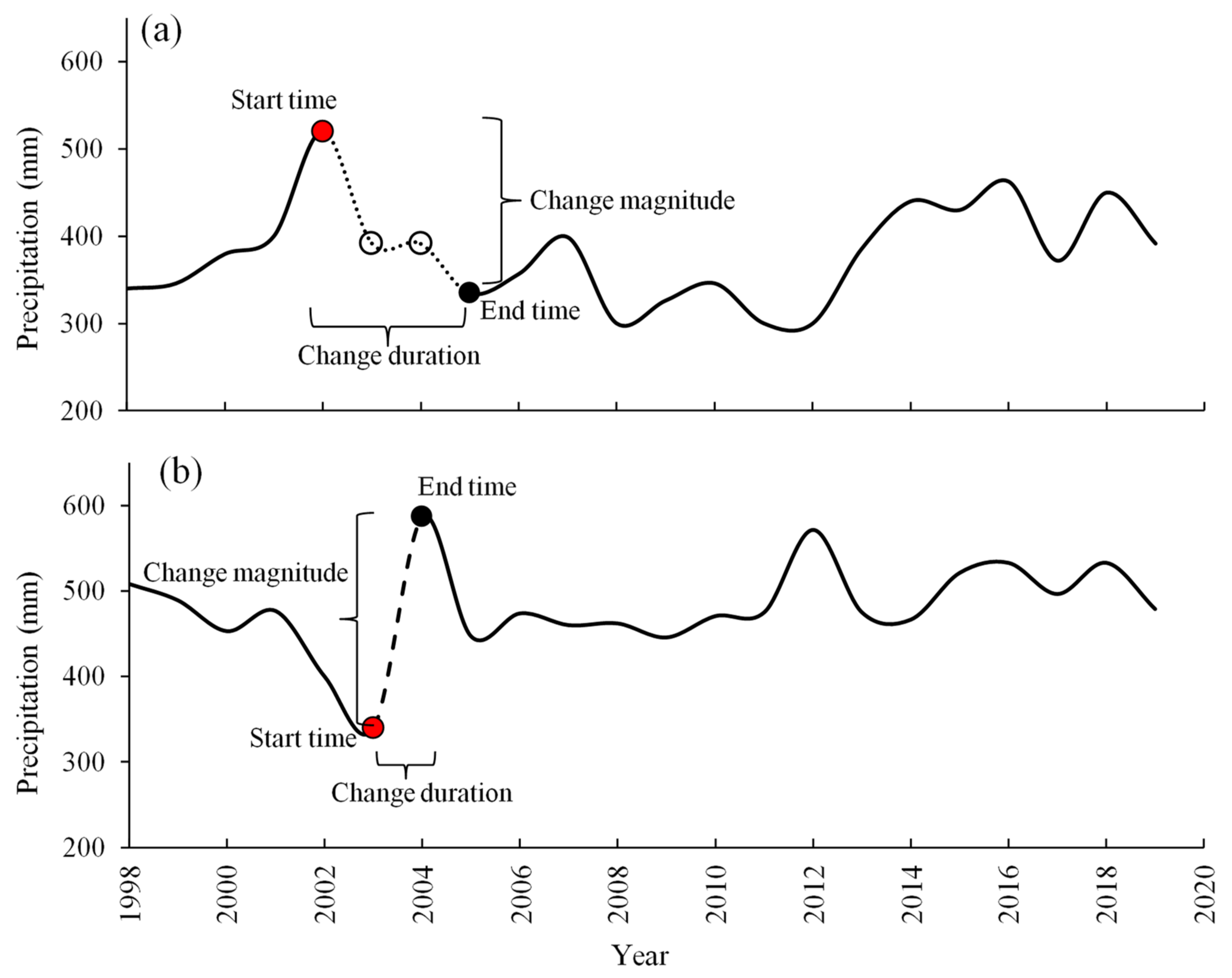
The trend direction changes for time points at which the valley/peak detector function equals one. These are called valley and peak points. For all datapoints, a second turning point detector function (g) is calculated based on the valley/peak detector function and an iterative criterion (refer to Jamali et al. [25]). Using this function, all potential turning points are identified (Figure 1). The identified level-shift points are added to the turning point set. For valid turning points, a subset of turning points that significantly reduces the residual sum of squares of a least-square fits the precipitation time series and does not result in overfitting, are then determined using an iterative piecewise fitting method based on Bayesian Information Criterion (BIC) [26]. The significance of the valid turning points is tested using statistical tests (α = 0.05) for the corresponding segments in the obtained optimal model fit to the precipitation trend that minimizes the BIC [25]. The significant turning points are called breakpoints (Figure 1). Note that a breakpoint can be abrupt or non-abrupt depending on whether it is a level-shift point or not, respectively. Finally, the magnitude and timing characteristics for the detected breakpoints are computed and reported as output for several of the greatest breakpoints of interest for detection set by the user (m = 1). For any detected change, the corresponding breakpoint (break date) is the start time, and the next turning point is the end time. The change duration is the time between the start time and the end time. The change magnitude is calculated by subtracting the fitted precipitation value at the start time from the fitted value at the end time (Figure 1). The sign of the obtained change value represents the change direction (whether the slope is decreasing or increasing); for more details, see Jamali et al. [25].
We used the DBEST algorithm for detecting and characterizing the greatest breakpoints in the TRMM TMPA 3B43 version 7 precipitation product, called the “TRMM and Other Data Precipitation Dataset’’ at a monthly time scale during the 1998–2019 period.

2.2.2. Data Preprocessing

Due to the large spatiotemporal variation in the global precipitation data (month-to-month and region-to-region), it is necessary to provide a meaningful measure of the interannual precipitation changes globally while preserving the relative difference of the observed precipitation at the pixel level. To remove the erroneous effects of scale differences on the change detection computation, we applied a pixel-based precipitation time series filter that accounts for two conditions. These conditions disregard precipitation changes of less than 1 mm and 0.05 median value over the study period. For example, the precipitation changes of 10 to 20% for the recorded event of below 1 mm may mathematically be considered significant, while in the conceptual interpretation this change does not represent a significant abrupt change or a breakpoint in the precipitation time series.
Accordingly, the first filter (Equation (4)), detects pixels for which the precipitation range over the studied 22-year period is less than 1 mm. Using this filter, the detected pixels are automatically discarded from DBEST analysis using the formula below:
Ri = Pi max− Pi min Ri < 1 mm at each pixel
where P is precipitation (mm), R is the precipitation range during the 22 years (1998–2019), and i is the pixel number.
The second filter (Equation (5)) discards the pixels with a precipitation range lower than 0.05 of their median value during the period using the formula below:
Ri = Pi max − Pi min Ri < 0.05 × Pi median
The 0.05 median value was selected based on the Intergovernmental Panel on Climate Change report [54], which suggests a precipitation change from −5 to +5% between successive years can be classified as ‘No change’. In addition, we used the median value instead of the average, as the median is less influenced by precipitation extremes.

2.2.3. Precipitation Changes at Global, Continental, and Climate Zone Scales

We investigated the precipitation breakpoints and compared their characteristics at a quasi-global scale, i.e., start year, duration, magnitude, abrupt and gradual change type. We conducted breakpoint analysis at the continental vs. global scales to obtain insight regarding the change characteristics on land vs. ocean areas. As precipitation changes based on climate zone rather than depending on continental boundaries, we also evaluated our results associated with different climate zones. Here, we used the world map of Köppen–Geiger climate classification to explore the relationship between precipitation breakpoint features and different climate zones. The Köppen–Geiger climate classification was published in 1900 by Wladimir Köppen and was updated by Rudolf Geiger in 1961. In the last version of this classification, five main climate zones at the global scale have been recognized, encompassing (i) warm temperate, (ii) equatorial, (iii) arid, (iv) snow, and (v) polar [55,56]. To find a likely relationship between precipitation variation and abrupt and non-abrupt changes, we also applied the coefficient of variation (CV) for each pixel during the 1998–2019 period. The CV is defined as the ratio of standard deviation and mean.
Note that the greatest change is considered (both decreasing and increasing) in precipitation during the selected period (22 years). Although a longer-period dataset may provide more insight concerning historical changes, we think it is interesting to focus on the recent greatest changes in precipitation over this period.

3. Results

3.1. Global Scale

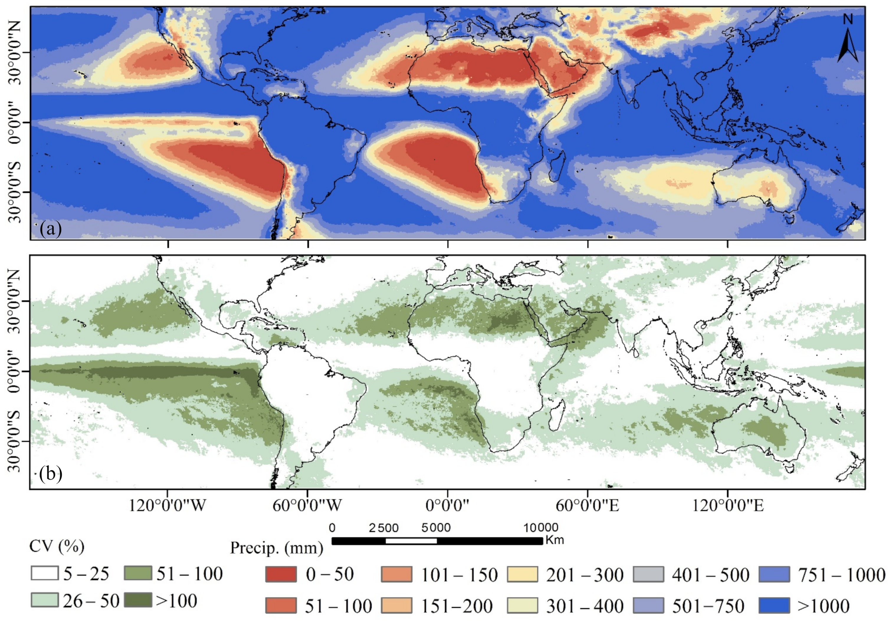
Figure 2 shows the annual 3B43 mean precipitation (mm) and coefficient of variation (CV%) in precipitation over the period studied. Precipitation at the global scale ranged from ~1 to more than 5000 mm in a year. While some portions of North Africa, Central Asia, North and South Pacific Oceans, and the South Atlantic Ocean received less than 100 mm over a year (Figure 2a), these regions exhibited the highest CV (>25%), indicating a high rate of variability in the annual precipitation (Figure 2b).
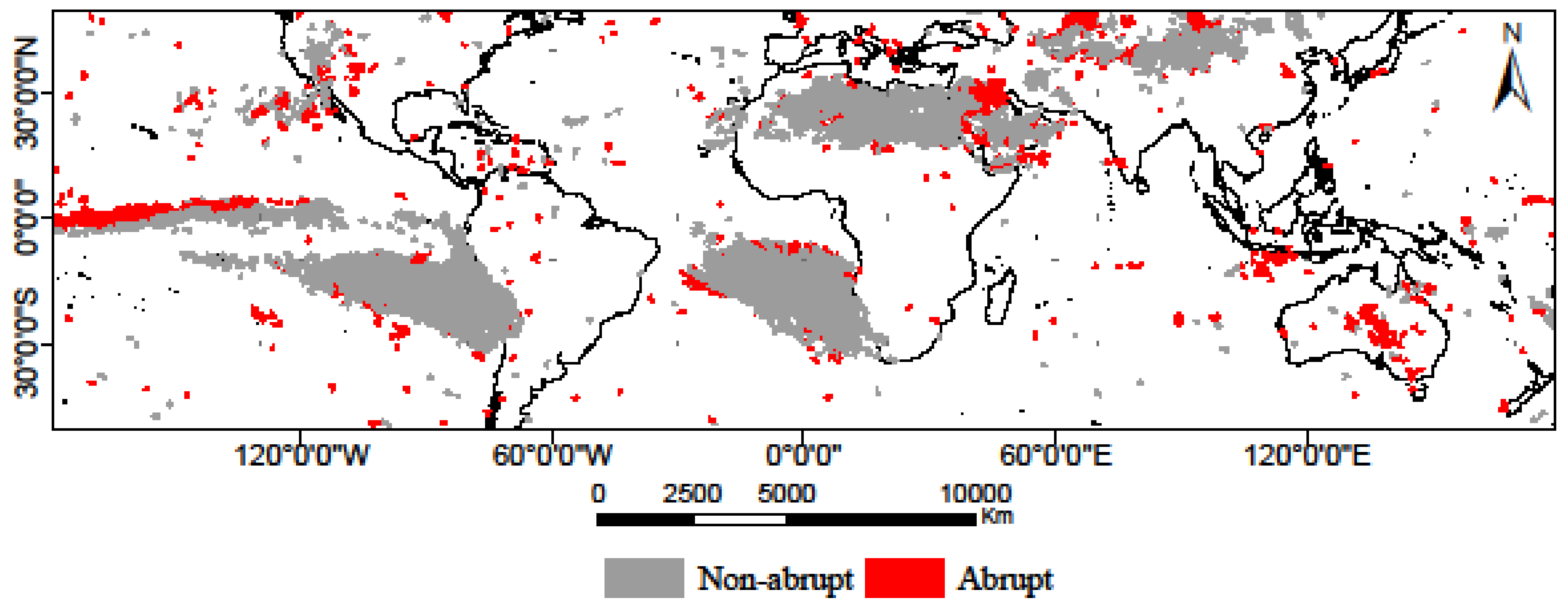
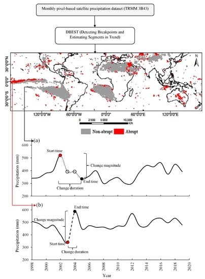
Figure 3 depicts the greatest breakpoints detected over the studied period. We found that 14.8% (85,217 pixels) of the entire study area experienced significant changes (abrupt and non-abrupt) in the recorded precipitation (0.05 significance level). An example of a typical abrupt and non-abrupt change in the global precipitation time series is depicted in Figure 4. In detail, we detected 9.4% non-abrupt changes, of which 6.3% occurred over the ocean, 3.1% over land, and 5.4% abrupt changes of which 3.6% occurred over the ocean and 1.8% over land.
The spatial coverage of non-abrupt changes for both ocean and land was considerably higher than abrupt changes (Figure 3). Most abrupt changes were found near the equator in the Pacific Ocean and Asia, relative to other ocean and land regions. Asia, North Africa, South Atlantic, and South Pacific Oceans experienced the highest frequency of breakpoints (abrupt and non-abrupt) in precipitation during the study period compared to the detected breakpoints over Australia, North Pacific, and Atlantic Oceans. Most breakpoints occurred in areas showing high CV (>25%) (Figure 2b and Figure 3). In contrast, we did not detect many breakpoints in regions with low CV, including regions with high precipitation amounts.
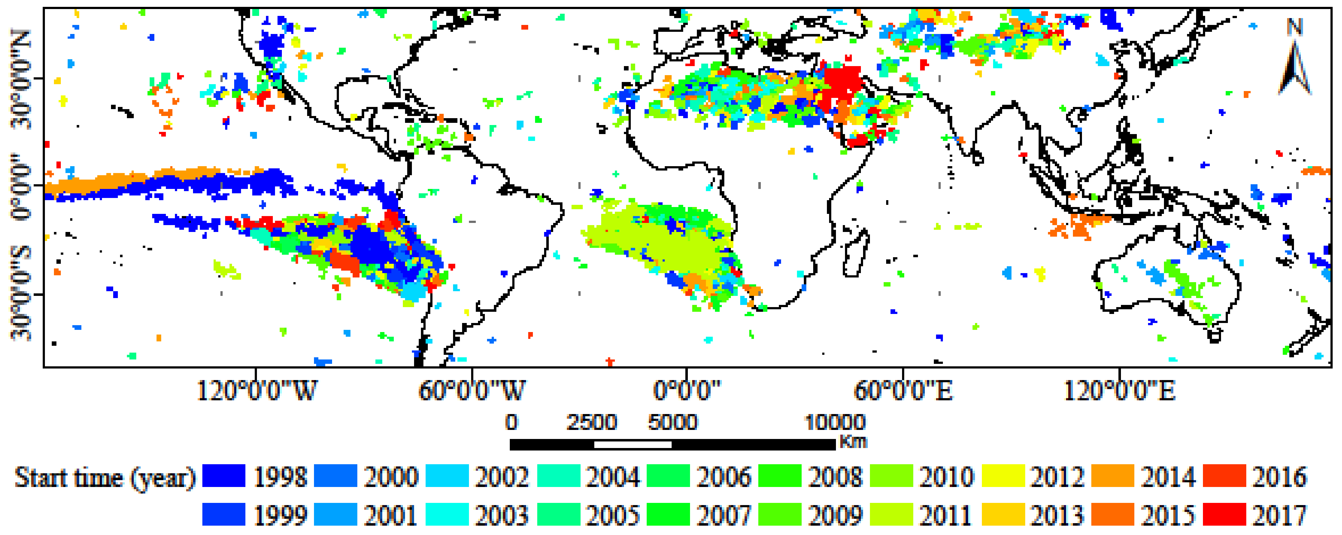
The majority of detected breakpoints, at a global scale, started during 1998, 1999, 2009, 2010, and 2011. Breakpoints in the South Pacific were mainly detected for 1998 and 1999 and in the South Atlantic for 2010 and 2011 (Figure 5). In overland areas, the breakpoints varied from 1998 to 2017.
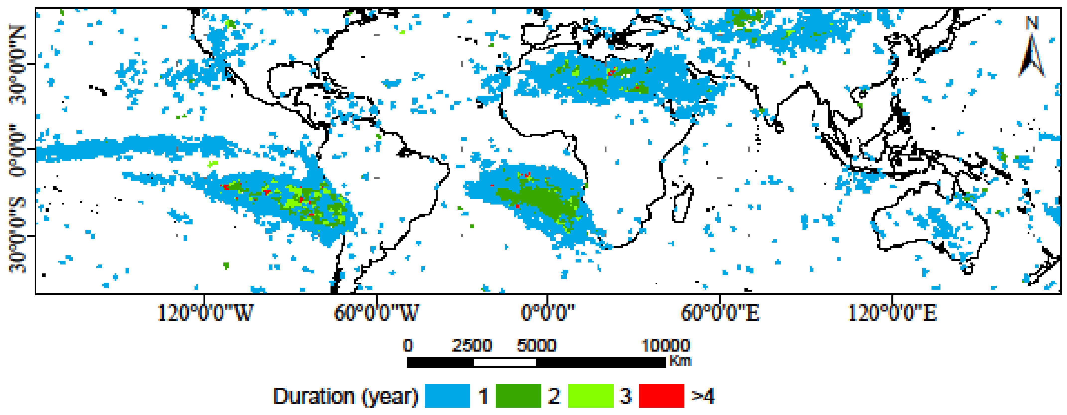
Figure 6 shows the change duration results (year) at the global scale. Most of the detected breakpoints, 73%, occurred during a relatively short (one-year) period. Approximately 16.8 and 7% of breakpoints occurred during a two- and three-year period, respectively. The remaining percentage, 3.2%, varied between four to nine years.
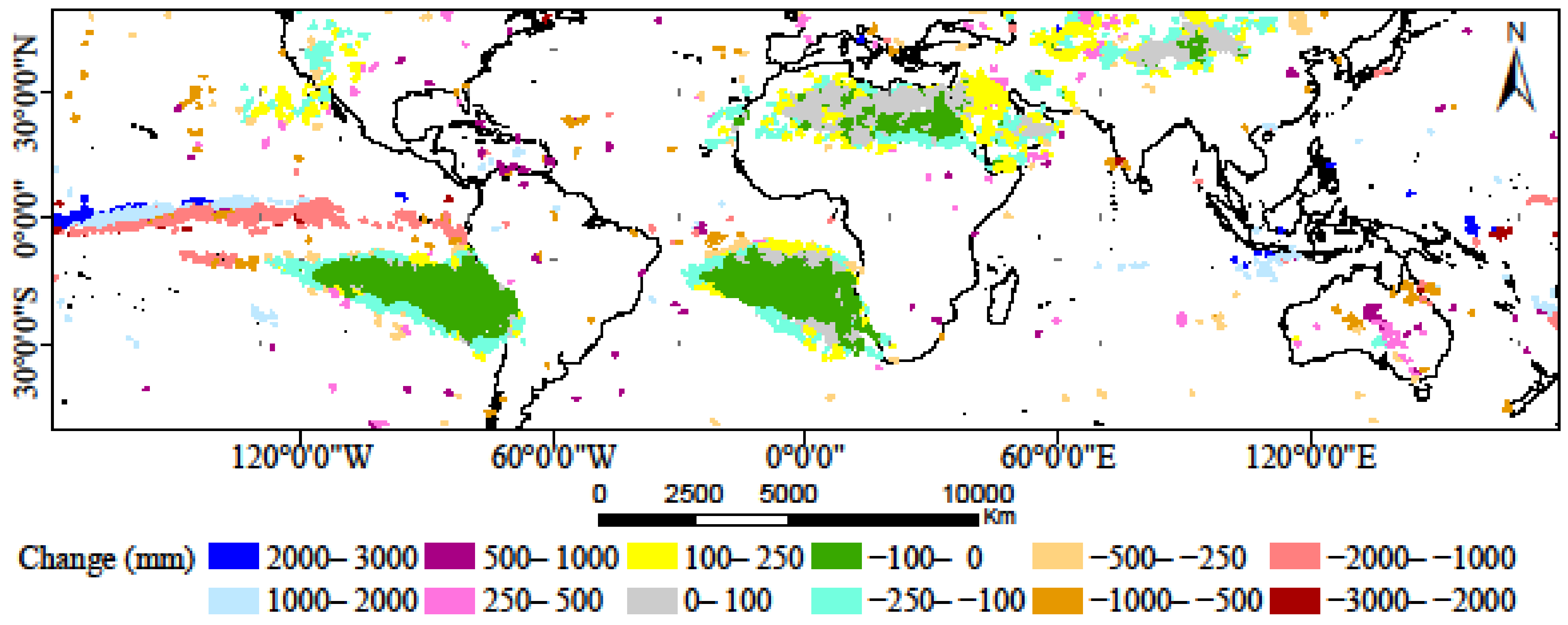
The magnitude of precipitation changes varied from −3000 to +3000 mm across the globe (Figure 7). The largest magnitudes were more related to ocean climate, especially near the equator of the Pacific Ocean (±2000 to ±3000 mm). Although the precipitation in some regions changed by ±3000 mm, most changes were approximately ±100 mm for the detected breakpoint duration. For instance, precipitation in most portions of Africa and Asia changed with a magnitude of +100 mm, including both abrupt and non-abrupt changes. In contrast, most changes over the South Pacific and South Atlantic Oceans occurred with a magnitude of −100 mm (Figure 7).

3.2. Continental Scale

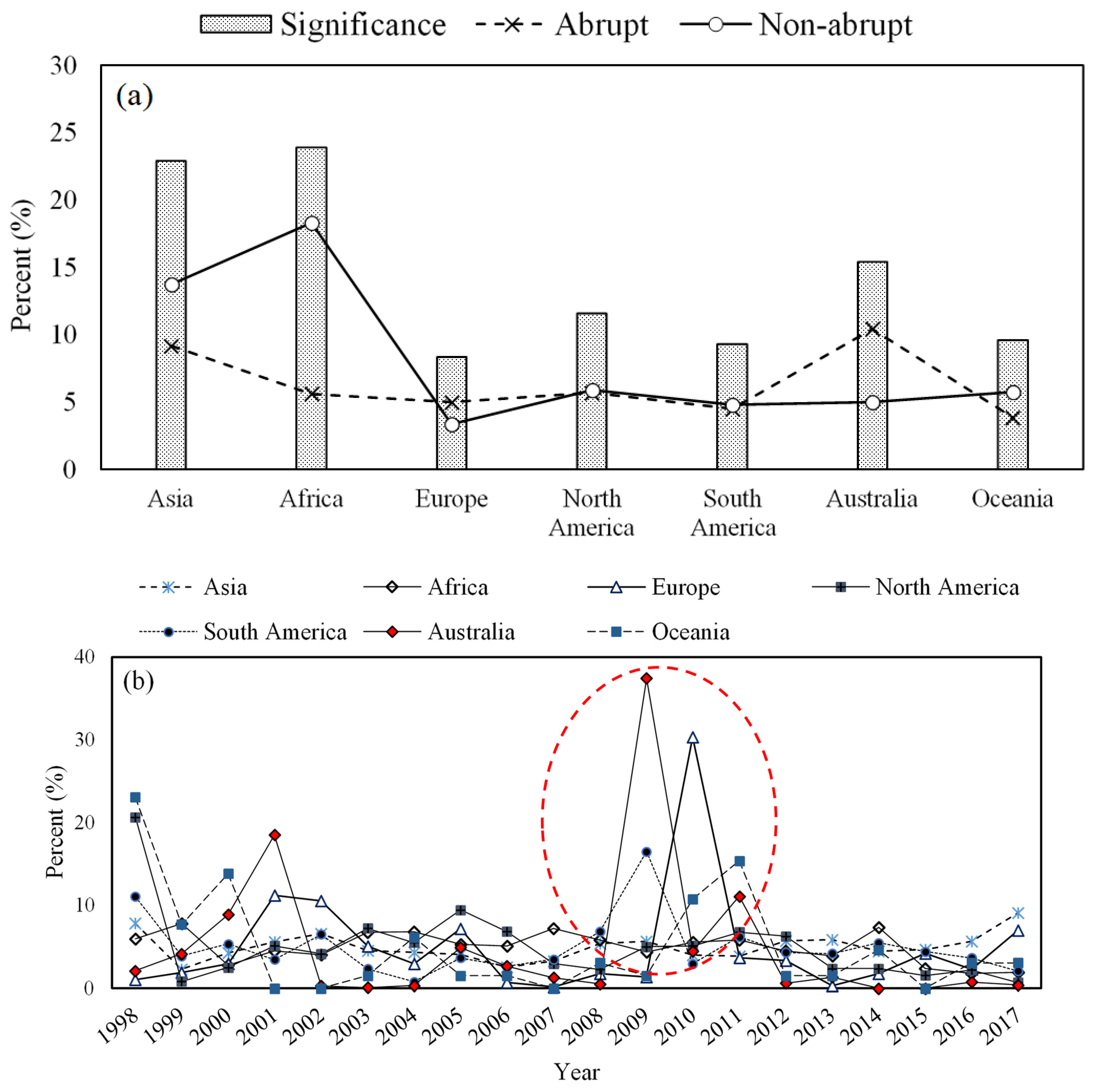
Significant abrupt and non-abrupt changes over the continents are depicted in Figure 8a. More significant breakpoints occurred over Africa (23.9%), Asia (22.9%), and Australia (15.4%) as compared to North America (11.6%), South America (9.3%), Europe (8.3%), and Oceania (9.6%). Further, there were more non-abrupt changes in Asia (13.7%) and Africa (18.3%) than there were abrupt changes (Asia: 9.1% and Africa: 5.6%) (Figure 3). Conversely, the percentage of abrupt changes occurring in Australia (10.4%) was more than that of non-abrupt changes (4.9%). In Africa, a majority of significant breakpoints occurred over the northern region of the continent, while in Asia it occurred in the western and central regions of the continent. In North and South America, significant breakpoints mainly extended over western regions of the continent (Figure 3).
Figure 8b shows the distribution of detected breakpoint occurrences for all continents over the study period. The results indicate that all detected breakpoints extended from 1998 through 2017. This means that we observed no breakpoints for 2018 and 2019. The detected breakpoints only extended during less than 25% of each year, except in Australia and Europe, where the breakpoints extended to 37.4 (during 2009) and 30.3% (during 2010), respectively. During 2009 and 2010, South America and Oceania also showed a high percentage of breakpoints relative to other continents. In the first year (1998), North America and Oceania had the highest proportion of breakpoints relative to other continents, extending over 23.1 and 20.7% of the year, respectively.
Results for significant positive and negative breakpoints over different continents are given in Table 2. The highest percentage of negative changes (abrupt and non-abrupt) was detected in Oceania (73.8%), Europe (61.8%), North America (56.2%), and South America (55.5%), while the lowest percentage was detected in Asia (41.7%) and Australia (46.9%). Asia, North Africa, and North and South America varied from −100 to +100 mm regarding the magnitude of change. The change value in Australia ranged from −1000 to +500 mm over the study period (Figure 7).

3.3. Climate Zone Scale

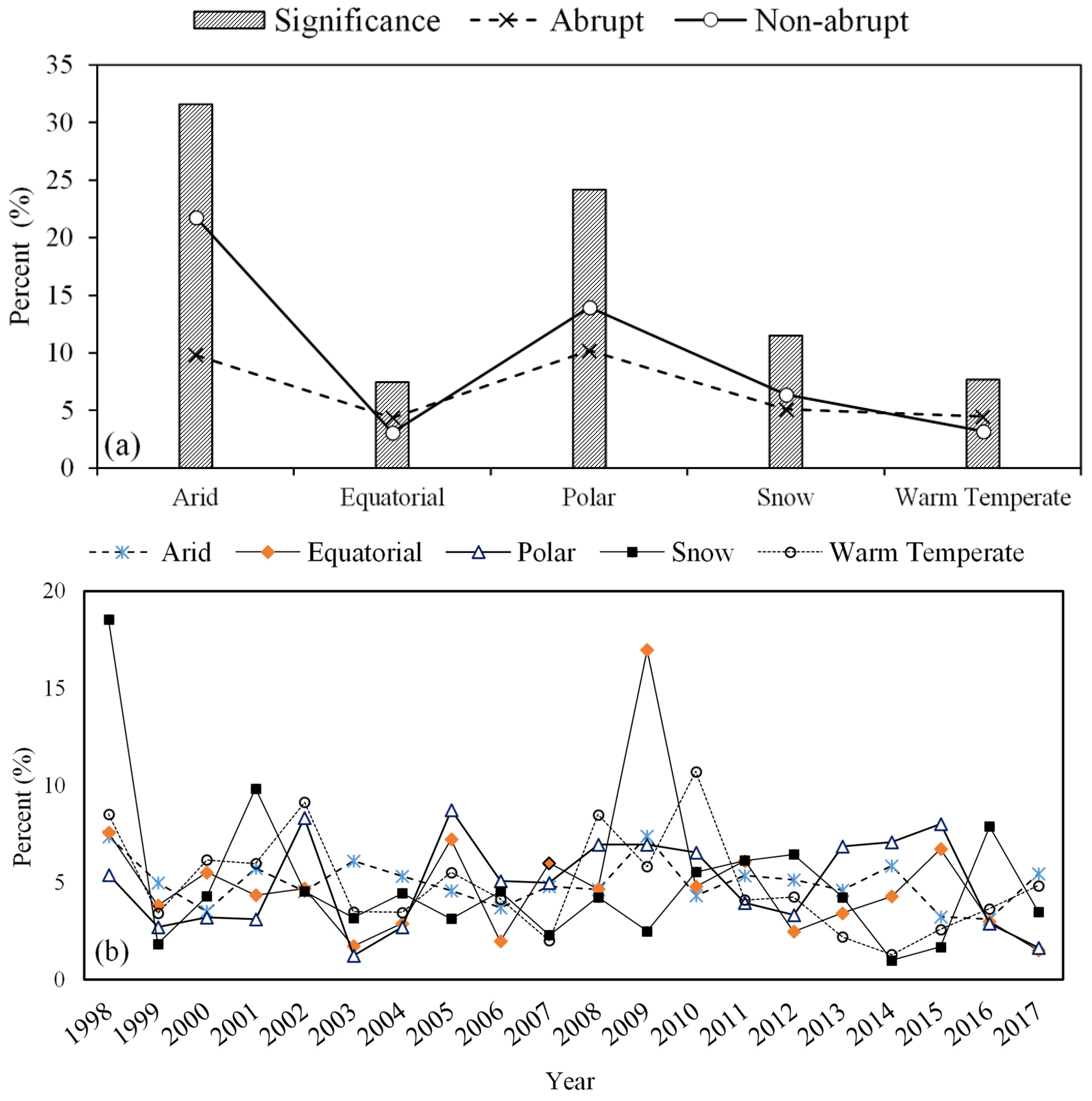
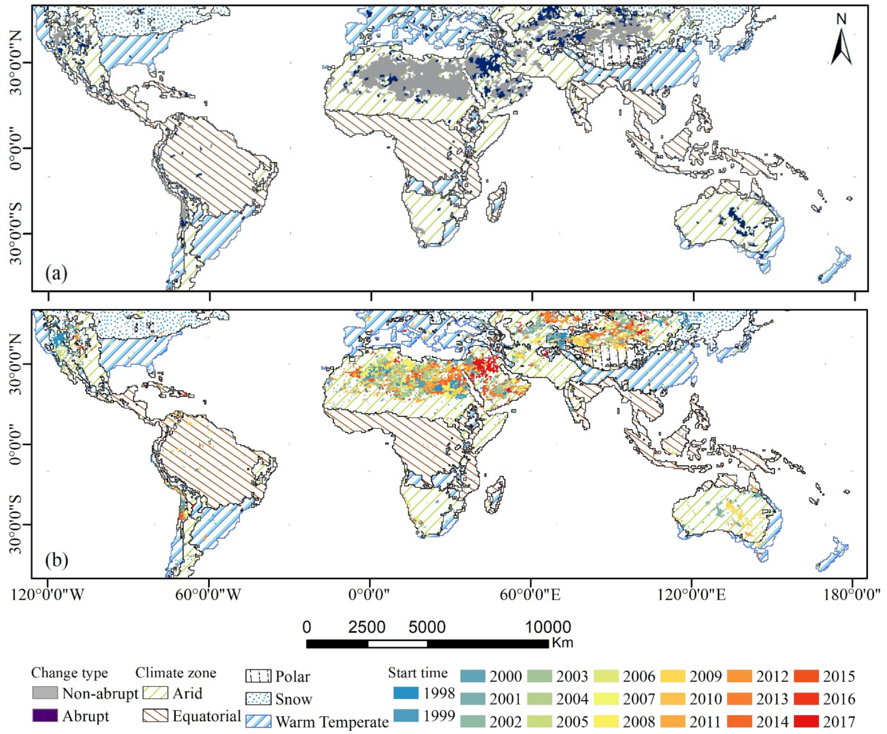
We observed that the most significant breakpoints occurred in arid (31.6%) and polar (24.1%) climates, while we found fewer breakpoint events in snow-covered areas (11.5%), equatorial (7.5%), and warm temperate (7.7%) climate zones (Figure 9a). The results of the change type indicated that the non-abrupt changes in arid (abrupt: 9.8%; non-abrupt: 21.7%) and polar (abrupt: 10.2%; non-abrupt: 13.9%) climates extended over a larger area compared to snow-covered regions (abrupt: 5.1%; non-abrupt: 6.4%), equatorial (abrupt: 4.4%; non-abrupt: 3.1%), and warm temperate (abrupt: 4.5%; non-abrupt: 3.2%) climate zones (Figure 9a). Figure 9b shows the breakpoint year for different climate zones. In principle, the results obtained for the start time indicated that breakpoints only occurred from 1998 to 2017 in different climate zones (Figure 9b) with approximately 10% for each year in all climate zones except equatorial and snow climates, which indicated a higher percentage (~17.5%) in 1998 and 2009 (Figure 10a,b). The results of durations revealed that most of the detected breakpoints (>85%) occurred over a one- to two-year period in different climate zones.
We detected higher percentages of positive breakpoints in arid (54%) and equatorial (51.9%) climates relative to those in other climate zones. Further, the highest percentage of negative breakpoints was found over the polar, snow-covered, and warm temperate climates, with approximately 55% each relative to other climate zones (Table 3).
According to Table 4, positive changes ranged from 3 to 2720 mm per year (on average, 164 mm), while negative changes varied from −2114 to −3 mm per year (on average, −174 mm) in the arid climate. The mean of positive and negative changes specified that most changes were lower than ±180 mm per year in the arid climate zone over the study period. Similarly, the average detected precipitation changes in the polar climate were 194 mm and −159 mm per year for the positive and negative changes, respectively. We found the greatest change in the equatorial climate zone, with a mean of 874 mm and −847 mm per year (variation from 3000 to −2998 mm) for positive and negative changes, respectively. The mean change for the snowy climate zone was +326 mm and −324 mm for the positive and negative changes, respectively. We found 574 mm and −634 mm of positive and negative precipitation changes per year in the warm temperate climate zone, respectively (Table 4).

4. Discussion

4.1. Precipitation Changes at Global Scale

Due to the great loss of human lives and exponentially increasing damage costs associated with extreme precipitation events, studying abrupt and non-abrupt changes in precipitation has received much attention in recent years [57] because it provides insight as to how climate extremes influence the ecosystem and society [57]. In addition, as the spatial distribution of precipitation is not limited to a particular region with a defined geopolitical boundary, such as cities, countries, and continents, it is necessary to conduct research considering spatial aggregation representing different climatological characteristics.
The CV is robust in detecting precipitation variability and changes [58]. In addition, significant deviations from mean annual precipitation (i.e., high CV) can cause significant stress to ecological and human systems [59]. Generally, high temporal variability in precipitation (month to month and year to year) is the leading cause of the detected changes. For instance, some portions of North Africa, Central Asia, the North and South Pacific Oceans, and the South Atlantic Ocean receive precipitation lower than 100 mm/year. At the same time, these regions have the highest CV (more than 25%). In addition, precipitation variability can increase over time. Dore [60] reported increased precipitation variance globally, with higher variability over the equatorial region.
On the global scale, the detected breakpoints in precipitation can be derived from significant shift changes with decreasing light precipitation and increasing heavy precipitation over time. Recently, researchers have reported that light precipitation events significantly decreased during the past decades on regional and global scales (e.g., [61,62,63,64]). For instance, Ma et al. [62] reported that very heavy precipitation (P ≥ 50 mm day−1) events have increased significantly from 1960 to 2013, while light (0.1 ≤ P < 10 mm day−1) and moderate (10 ≤ P < 25 mm day−1) events have decreased significantly in China. This indicates a shift from light to intense precipitation, implying increased risks of drought and floods [62]. Additionally, increasing heavy precipitation events can cause significant abrupt and non-abrupt changes in precipitation. It is noteworthy to clarify that the abrupt and non-abrupt changes in precipitation can also be due to various local and regional natural and human impacts, including changes in the environment, measurement techniques, observation locations, and equipment [12].
Our findings indicated that most of the detected breakpoints, abrupt and non-abrupt changes, occurred over the land area in the Northern Hemisphere. In contrast, in the Southern Hemisphere, they occurred over the oceans. The most significant breakpoints in the Northern Hemisphere were found over Asia and North Africa (dry regions). In contrast, the highest percentage of breakpoints in the Southern Hemisphere was detected near the Equator in the South Pacific and South Atlantic, wet regions. Most breakpoints occurred in areas with low precipitation and high CV, which could be due to internal and external environmental factors. Conversely, we found no significant breakpoints in regions with low CV (including regions with high precipitation). This means that some dry regions (i.e., North Africa and Asia) and wet regions (i.e., South Pacific and South Atlantic) with high CV showed significant breakpoints in precipitation and can be expected to experience more extreme events due to climate change, and this intensification can lead to increased risk of floods, soil erosion, and droughts [64].
Although there is considerable variability in spatial trend patterns, observations suggest that the number of extreme precipitation events has increased globally (e.g., [4,6,9,65]), hence generating the greatest changes in precipitation. We found a high number of breakpoints during the 1998–1999 and 2009–2011 periods across the globe. Over the South Pacific Ocean, we detected more breakpoints in 1998 and 1999, while in the South Atlantic a similar number of breakpoints was found in 2010 and 2011. A warmer tropical Pacific in 1998 was caused by a positive El Niño Southern Oscillation (ENSO) event [60]. ENSO influences precipitation changes at the global scale [66,67,68,69,70] and is related to the variations of temperature and precipitation over much of the sub-tropics and tropics, as well as some mid-latitude regions [60]. In line with the detected breakpoint years related to ENSO, a global increase in surface temperature for El Niños (1998 and 2010) and negative global anomalies during La Niñas (1999–2001) have been reported. The maximum amplitude of surface temperature occurred during the 1998 El Nino (~+0.15 °C), with a lower amplitude (negative) during La Nina, 1999–2001. Moreover, during the cold (warm) phase of ENSO, La Niña (El Niño), most of the tropical ocean surfaces are cooler (warmer) than normal, and the atmosphere is charged with less (more) moisture, resulting in less (more) extreme precipitation events over the (combined ocean and land) tropical region [66,69]. Higher surface temperature leads to a greater evaporation rate (especially over the ocean and overtime) and a greater instability, hence impacting the variation of large-scale precipitation [3]. Lausier and Jain [59] reported that sea surface temperature variability patterns were strongly correlated with global precipitation patterns during the period 1951–2011, helping to drive variability in annual precipitation. Adler et al. [3] stated that the ocean shows the opposite anomaly compared to the land areas for ENSO.
Regarding the large El Niño during 1998, positive and negative anomalies occurred over the ocean and land areas, respectively. This is due to the pattern of positive rainfall anomalies over the tropics, particularly the central and eastern Pacific Oceans, which could be a reason for the detected breakpoints in the land regions versus ocean areas in our study. These reported results, along with our findings, have already been addressed in both climate simulations and satellite observations [66,69], indicating that ENSO is a dominant driver of precipitation extremes in the tropics [69].
Our findings indicate that the change in magnitude of precipitation notably occurred over the oceans, especially near the Equator in the Pacific Ocean. Analyses of the Climate Prediction Center (CPC) Merged Analysis of Precipitation (CMAP) product [71] and the National Centers for Environmental Prediction (NCEP) reanalysis project [72] show that there have been substantial increases in average precipitation over the tropical oceans, related to the increased intensity and frequency of ENSO during the period 1979–1998 [2]. Similarly, we found a substantial spatial coverage of breakpoints, abrupt and non-abrupt, occurring over Asia, North Africa, South Atlantic, and South Pacific Oceans. Moreover, the detected breakpoints revealed that a decreasing precipitation trend impacted some parts of the subtropics and tropics compared to other regions. Likewise, Trenberth et al. [73] reported a noticeable change in precipitation pattern in recent years, suggesting a wetter condition for the high latitudes and a drier condition for the subtropics and tropics, which is associated with the large-scale precipitation change influenced by ENSO [74]. Further, our findings indicated that the Indian and North Atlantic Oceans experienced the lowest number of breakpoint occurrences in precipitation over the study period. This is contrary to findings by Pokhrel et al. [75], who used Objectively Analyzed air-sea Fluxes (OAFlux) and the latest version of National Centers for Environment Prediction (NCEP) Climate Forecast System (CFS) version-2 products. They reported significant precipitation variability and changes over the Indian Ocean affected by El Niño and La Niña signals during the earlier period, 1979–2010, which partially overlaps the period of the current study. This contradiction could be due to the usage of several variables such as evaporation-precipitation (E-P), wind speed, air-sea humidity, and sea surface temperature (SST), which was different from the only precipitation variable used in this study. The past time series (<1998) were not available, but the changes in precipitation between 1998 and 1999 and subsequent years (>1999) were abrupt, which were considered breakpoints in our study. More importantly, the detected that breakpoints during the 1998–1999 period were more reasonable than other years’ changes due to the reported substantial increases in average precipitation over the tropical oceans, related to the increased intensity and frequency of ENSO during the period 1979–1998 [2].

4.2. Precipitation Changes at the Continental and Climate Scales

We detected a higher frequency of breakpoints over Africa, Asia, and Australia relative to other continents. Not only the spatial coverage of non-abrupt changes for both ocean and land was considerably higher than abrupt changes but also the detected non-abrupt changes in Asia and Africa were more than that of abrupt changes. This means that the magnitude of precipitation changes in these regions was low. Although we found a large number of breakpoints over some regions of Asia and Africa, we detected the lowest changes in the magnitude of precipitation (±100 mm), which is due to the high CV in these regions (i.e., low precipitation amount but high precipitation variability). These breakpoints could be related to the observed extreme rainfall events, especially over north tropical Asia, around 10–20°N, [76].
Major precipitation and severe drought occurrences can be related to positive and negative breakpoints, respectively. Frequent severe drought and flood events, especially in the central region of Asia, during the past decades have been reported [64,67], which agrees with the spatial distribution of the detected breakpoints over Asia in this study. Moreover, an increase of 1.3 °C in average temperature over Asia, particularly China, with increased evaporation has led to extreme regional precipitation and observed breakpoints (e.g., [77,78,79,80]). In North and South America, we found significant breakpoints extending over western regions of the continents. The changes in extreme precipitation and duration are likely to result from the combined effects of large-scale circulation changes and climate change. Climate change may affect the probability and intensity of extreme weather events [66,78], as it can be the main reason for breakpoints in precipitation.
Regarding climate zones, we found that the majority of significant breakpoints occurred over the arid and polar climates, relative to other climate zones. Our findings indicate that detected breakpoints in precipitation over the arid climate were mainly positive (upward) compared to other climate zones (i.e., Asia and Africa). To address this observation, it is noted that the arid climate is characterized by limited precipitation with a high spatial and temporal variation that explains the higher density of the detected breakpoints over this zone [81,82,83]. The change in the average precipitation in arid climates specified that the majority of breakpoints were detected in the range between −180 and +180 mm over the studied period. Conversely, we found minor breakpoints in the equatorial and warm temperate (<8%) climate zones. Based on the climate classification scheme, the equatorial climate mainly covers central Africa, northern regions of South America, southern India, Sri Lanka, northern Australia, Indonesia, Thailand, Vietnam, Malaysia, Laos, Philippines, Myanmar, and most Pacific Island nations. It seems that the equatorial climate, with a high humidity regime, provides a low variability, which can be the main reason for detecting fewer breakpoints. For example, the equatorial climate of Central Africa sustains tropical rainforests throughout the region and provides the excellent growing conditions needed for high-value crops [84].
Our findings indicate that high precipitation variability is the leading cause of significant breakpoints. Precipitation variability is a crucial climatic factor for the environment, agriculture, and society. Increased precipitation variability can reduce agricultural yield [85] and affect development [86,87]. This connects extreme dry and wet events, droughts, and floods, posing threats to society and the environment [86,88]. Much more attention needs to be given to regions with many abrupt changes to mitigate the impact of extreme natural events such as droughts and floods derived from climate extremes. Therefore, this study provides essential information to pinpoint the areas under frequent precipitation changes at the quasi-global and continental scales and their associations with the climate zones. Finally, theoretical and practical research is required to connect the understanding of changes in precipitation, and the threats they pose to the environment and society.

5. Conclusions

To decrease the impacts of floods and droughts, there is a vital need to study historical events, i.e., breakpoints in precipitation, at the global scale. Although there are several studies concerning precipitation changes, breakpoints, and trends, on a regional scale using common statistical tests, conducting a comprehensive global investigation on the greatest changes in precipitation is of great importance. We used the DBEST algorithm for analyzing precipitation change and its characteristics in a monthly satellite-based precipitation dataset (TRMM 3B43) at three different scales: (i) global, (ii) continental, and (iii) climate zone over the 1998–2019 period. Unlike previous studies on precipitation changes at the local and regional scales, this study focused on quasi-global scale precipitation to detect general patterns of both abrupt and non-abrupt changes. This helps better understand the changes in overall precipitation patterns and adequately develop a mitigation strategy for future likely extreme event impacts.
The output of the DBEST algorithm captured the type (non-abrupt or abrupt) and characteristics (magnitude and time) of the significant breakpoints observed in satellite-based precipitation time series. We found 14.1% abrupt and non-abrupt significant breakpoints in the quasi-global precipitation dataset (0.05 significance level). The highest percentage of abrupt changes was found near the equator in the Pacific Ocean and Asia, relative to other oceans and land regions. On the continental scale, the detected breakpoints in Africa (23.9%), Asia (22.9%), and Australia (15.4%) were more than those in North America (11.6%), South America (9.3%), Europe (8.3%), and Oceania (9.6%). The findings indicate that the most significant breakpoints were found in the arid (31.6%) and polar (24.1%) climates on the climate zone scale. The detected breakpoints in precipitation are more likely to be related to the extreme wet and dry events associated with ENSO and high precipitation variability. However, these results indicate that abrupt changes in precipitation differ not only between regions but also in different aspects of precipitation, i.e., total and extreme.
The consequences of precipitation variability and change, substantial changes, affect water resources at the local to regional scale where crops are grown, people live, and industrial and agricultural water requirements for production purposes exist. Our findings indicate that larger parts of Africa and Asia experienced a significant number of the most extensive changes in precipitation. Compared to the average state (trend during a specific period), the greatest changes in precipitation in these regions were more abrupt, which may pose a severe threat to the ecology, environment, and natural resources, causing a substantial loss in urban and rural areas.
In conclusion, this study provides a large-scale comprehensive perspective of abrupt and non-abrupt precipitation changes over the global, continental, and climate zone during the 1998–2019 period. The monthly satellite pixel-based precipitation dataset (TRMM 3B43) provided valuable information to address the precipitation change characteristics during the last two decades. The DBEST algorithm detected and quantified the major changes in precipitation over large areas at continental and global scales. While applying this algorithm in the precipitation studies, it is suggested that this algorithm be implemented using other climate variables. It is a flexible, accurate, and fast tool for change detection, and is applicable to global change studies using time series of satellite-based datasets.

Author Contributions

Conceptualization, methodology, writing—original draft preparation, software, validation, M.K.; conceptualization, supervision, methodology, writing—reviewing and editing, H.H.; conceptualization, methodology, software, writing—reviewing and editing, S.J.; writing—reviewing and editing, C.B.U., R.B. and G.J.H. All authors have read and agreed to the published version of the manuscript.

Funding

This research received no external funding.

Data Availability Statement

Data are available from the Tropical Rainfall Measuring Mission (TRMM) datasets. (https://disc.gsfc.nasa.gov/datasets/TRMM_3B43_7/summary, accessed on 1 February 2020).

Acknowledgments

The authors would like to thank the National Aeronautics and Space Administration (NASA) and the Japan Aerospace Exploration Agency (JAXA) for providing the Tropical Rainfall Measuring Mission (TRMM) datasets. The 3B43 data can be downloaded at https://disc.gsfc.nasa.gov/datasets/TRMM_3B43_7/summary, accessed on 1 February 2020.

Conflicts of Interest

The authors declare no conflict of interest.

References

  1. Longobardi, A.; Villani, P. Trend analysis of annual and seasonal rainfall time series in the Mediterranean area. Int. J. Climatol. 2010, 30, 1538–1546. [Google Scholar] [CrossRef]
  2. Trenberth, K.E. Changes in precipitation with climate change. Clim. Res. 2011, 47, 123–138. [Google Scholar] [CrossRef] [Green Version]
  3. Adler, R.F.; Gu, G.; Sapiano, M.; Wang, J.-J.; Huffman, G.J. Global precipitation: Means, variations and trends during the satellite era (1979–2014). Surv. Geophys. 2017, 38, 679–699. [Google Scholar] [CrossRef] [Green Version]
  4. Donat, M.G.; Lowry, A.L.; Alexander, L.V.; O’Gorman, P.A.; Maher, N. Addendum: More extreme precipitation in the world’s dry and wet regions. Nat. Clim. Change 2017, 7, 154–158. [Google Scholar] [CrossRef] [Green Version]
  5. Alexander, L.V.; Zhang, X.; Peterson, T.C.; Caesar, J.; Gleason, B.; Klein Tank, A.; Haylock, M.; Collins, D.; Trewin, B.; Rahimzadeh, F. Global observed changes in daily climate extremes of temperature and precipitation. J. Geophys. Res. Atmos. 2006, 111, 1042–1063. [Google Scholar] [CrossRef] [Green Version]
  6. Westra, S.; Alexander, L.V.; Zwiers, F.W. Global increasing trends in annual maximum daily precipitation. J. Clim. 2013, 26, 3904–3918. [Google Scholar] [CrossRef] [Green Version]
  7. Kharin, V.V.; Zwiers, F.W.; Zhang, X.; Wehner, M. Changes in temperature and precipitation extremes in the CMIP5 ensemble. Clim. Change 2013, 119, 345–357. [Google Scholar] [CrossRef]
  8. Sillmann, J.; Kharin, V.V.; Zwiers, F.; Zhang, X.; Bronaugh, D. Climate extremes indices in the CMIP5 multimodel ensemble: Part 2. Future climate projections. J. Geophys. Res. Atmos. 2013, 118, 2473–2493. [Google Scholar] [CrossRef]
  9. Donat, M.; Alexander, L.V.; Yang, H.; Durre, I.; Vose, R.; Dunn, R.J.; Willett, K.M.; Aguilar, E.; Brunet, M.; Caesar, J. Updated analyses of temperature and precipitation extreme indices since the beginning of the twentieth century: The HadEX2 dataset. J. Geophys. Res. Atmos. 2013, 118, 2098–2118. [Google Scholar] [CrossRef] [Green Version]
  10. Zhang, S.H.; Zhang, P.Y. Abrupt change study in climate change. Adv. Earth Sci. 1989, 3, 47–54. [Google Scholar]
  11. Buishand, T. Tests for detecting a shift in the mean of hydrological time series. J. Hydrol. 1984, 73, 51–69. [Google Scholar] [CrossRef]
  12. Reeves, J.; Chen, J.; Wang, X.; Lund, R.; Lu, Q. A review and comparison of climate control data for climate data. J. Appl. Meteorol. Clim. 2007, 46, 900–915. [Google Scholar] [CrossRef]
  13. Zhao, C.; Cui, Y.; Zhou, X.; Wang, Y. Evaluation of performance of different methods in detecting abrupt climate changes. Discret. Dyn. Nat. Soc. 2016, 2016, 5898697. [Google Scholar] [CrossRef] [Green Version]
  14. Lund, R.; Reeves, J. Detection of undocumented changepoints: A revision of the two-phase regression model. J. Clim. 2002, 15, 2547–2554. [Google Scholar] [CrossRef]
  15. Seidou, O.; Ouarda, T.B. Recursion-based multiple changepoint detection in multiple linear regression and application to river streamflows. Water Resour. Res. 2007, 43, W07404. [Google Scholar] [CrossRef] [Green Version]
  16. Wang, X.L. Comments on “Detection of undocumented changepoints: A revision of the two-phase regression model”. J. Clim. 2003, 16, 3383–3385. [Google Scholar] [CrossRef]
  17. Worsley, K. On the likelihood ratio test for a shift in location of normal populations. J. Am. Stat. Assoc. 1979, 74, 365–367. [Google Scholar]
  18. Buishand, T.A. Some methods for testing the homogeneity of rainfall records. J. Hydrol. 1982, 58, 11–27. [Google Scholar] [CrossRef]
  19. Pettitt, A.N. A non-parametric approach to the change-point problem. J. R. Stat. Soc. Ser. C 1979, 28, 126–135. [Google Scholar] [CrossRef]
  20. Alexandersson, H. A homogeneity test applied to precipitation data. J. Climatol. 1986, 6, 661–675. [Google Scholar] [CrossRef]
  21. Hsu, K.-C.; Li, S.-T. Clustering spatial–temporal precipitation data using wavelet transform and self-organizing map neural network. Adv. Water Resour. 2010, 33, 190–200. [Google Scholar] [CrossRef]
  22. Vincent, L.A. A technique for the identification of inhomogeneities in Canadian temperature series. J. Clim. 1998, 11, 1094–1104. [Google Scholar] [CrossRef]
  23. Kazemzadeh, M.; Malekian, A. Homogeneity analysis of streamflow records in arid and semi-arid regions of northwestern Iran. J. Arid Land 2018, 10, 493–506. [Google Scholar] [CrossRef] [Green Version]
  24. McCuen, R.H. Modeling Hydrologic Change: Statistical Methods; CRC Press: Boca Raton, FL, USA, 2016. [Google Scholar]
  25. Jamali, S.; Jönsson, P.; Eklundh, L.; Ardö, J.; Seaquist, J. Detecting changes in vegetation trends using time series segmentation. Remote Sens. Environ. 2015, 156, 182–195. [Google Scholar] [CrossRef]
  26. Schwarz, G. Estimating the dimension of a model. Ann. Stat. 1978, 6, 461–464. [Google Scholar] [CrossRef]
  27. Rousseeuw, P.J.; Leroy, A.M. Robust Regression and Outlier Detection; John Wiley & Sons Inc.: New York, NY, USA, 1987. [Google Scholar]
  28. Lenderink, G.; Van Meijgaard, E. Increase in hourly precipitation extremes beyond expectations from temperature changes. Nat. Geosci. 2008, 1, 511–514. [Google Scholar] [CrossRef]
  29. O’Gorman, P.A. Sensitivity of tropical precipitation extremes to climate change. Nat. Geosci. 2012, 5, 697–700. [Google Scholar] [CrossRef]
  30. Huffman, G.; Adler, R.; Bolvin, D.; Gu, G.; Nelkin, E.; Bowman, K.; Hong, Y.; Stocker, E.; Wolff, D. The TRMM multi-satellite precipitation analysis: Quasi-global, multi-year, combined sensor precipitation estimates at fine scales. J. Hydrometeorol. 2007, 8, 28–55. [Google Scholar] [CrossRef]
  31. Kummerow, C.; Simpson, J.; Thiele, O.; Barnes, W.; Chang, A.; Stocker, E.; Adler, R.; Hou, A.; Kakar, R.; Wentz, F. The status of the Tropical Rainfall Measuring Mission (TRMM) after two years in orbit. J. Appl. Meteorol. 2000, 39, 1965–1982. [Google Scholar] [CrossRef]
  32. Huffman, G.J.; Adler, R.F.; Bolvin, D.T.; Nelkin, E.J. The TRMM multi-satellite precipitation analysis (TMPA). In Satellite Rainfall Applications for Surface Hydrology; Springer: Berlin/Heidelberg, Germany, 2010; pp. 3–22. [Google Scholar]
  33. Belete, M.; Deng, J.; Wang, K.; Zhou, M.; Zhu, E.; Shifaw, E.; Bayissa, Y. Evaluation of satellite rainfall products for modeling water yield over the source region of Blue Nile Basin. Sci. Total Environ. 2020, 708, 134834. [Google Scholar] [CrossRef]
  34. Huffman, G.J.; Bolvin, D.T.; Braithwaite, D.; Hsu, K.-L.; Joyce, R.J.; Kidd, C.; Nelkin, E.J.; Sorooshian, S.; Stocker, E.F.; Tan, J. Integrated multi-satellite retrievals for the global precipitation measurement (GPM) mission (IMERG). In Satellite Precipitation Measurement; Springer: Berlin/Heidelberg, Germany, 2020; pp. 343–353. [Google Scholar]
  35. Huffman, G.J.; Bolvin, D.T. TRMM and Other Data Precipitation Data Set Documentation; NASA: Greenbelt, MD, USA, 2013; Volume 28.
  36. Huffman, G.J. The Transition in Multi-Satellite Products from TRMM to GPM (TMPA to IMERG). 2016. Algorithm Information Document. Available online: https://docserver.gesdisc.eosdis.nasa.gov/public/project/GPM/TMPA-to-IMERG_transition.pdf (accessed on 2 November 2021).
  37. Kazemzadeh, M.; Hashemi, H.; Jamali, S.; Uvo, C.B.; Berndtsson, R.; Huffman, G.J. Linear and Nonlinear Trend Analyzes in Global Satellite-Based Precipitation, 1998–2017. Earths Future 2021, 9, e2020EF001835. [Google Scholar] [CrossRef]
  38. Hashemi, H.; Fayne, J.; Lakshmi, V.; Huffman, G.J. Very high resolution, altitude-corrected, TMPA-based monthly satellite precipitation product over the CONUS. Sci. Data 2020, 7, 74. [Google Scholar] [CrossRef] [PubMed]
  39. Hashemi, H.; Nordin, M.; Lakshmi, V.; Huffman, G.J.; Knight, R. Bias correction of long-term satellite monthly precipitation product (TRMM 3B43) over the conterminous United States. J. Hydrometeorol. 2017, 18, 2491–2509. [Google Scholar] [CrossRef]
  40. Prat, O.P.; Nelson, B.R. Characteristics of annual, seasonal, and diurnal precipitation in the Southeastern United States derived from long-term remotely sensed data. Atmos. Res. 2014, 144, 4–20. [Google Scholar] [CrossRef]
  41. Qiao, L.; Hong, Y.; Chen, S.; Zou, C.B.; Gourley, J.J.; Yong, B. Performance assessment of the successive Version 6 and Version 7 TMPA products over the climate-transitional zone in the southern Great Plains, USA. J. Hydrol. 2014, 513, 446–456. [Google Scholar] [CrossRef]
  42. Zhao, T.; Yatagai, A. Evaluation of TRMM 3B42 product using a new gauge-based analysis of daily precipitation over China. Int. J. Climatol. 2014, 34, 2749–2762. [Google Scholar] [CrossRef]
  43. Brown, J.E. An analysis of the performance of hybrid infrared and microwave satellite precipitation algorithms over India and adjacent regions. Remote Sens. Environ. 2006, 101, 63–81. [Google Scholar] [CrossRef]
  44. Mondal, A.; Lakshmi, V.; Hashemi, H. Intercomparison of trend analysis of multisatellite monthly precipitation products and gauge measurements for river basins of India. J. Hydrol. 2018, 565, 779–790. [Google Scholar] [CrossRef]
  45. Prakash, S.; Mitra, A.K.; Pai, D.; AghaKouchak, A. From TRMM to GPM: How well can heavy rainfall be detected from space? Adv. Water Resour. 2016, 88, 1–7. [Google Scholar] [CrossRef]
  46. Huang, Y.; Chen, S.; Cao, Q.; Hong, Y.; Wu, B.; Huang, M.; Qiao, L.; Zhang, Z.; Li, Z.; Li, W. Evaluation of version-7 TRMM multi-satellite precipitation analysis product during the Beijing extreme heavy rainfall event of 21 July 2012. Water 2013, 6, 32–44. [Google Scholar] [CrossRef] [Green Version]
  47. Li, X.-H.; Zhang, Q.; Xu, C.-Y. Suitability of the TRMM satellite rainfalls in driving a distributed hydrological model for water balance computations in Xinjiang catchment, Poyang lake basin. J. Hydrol. 2012, 426, 28–38. [Google Scholar] [CrossRef]
  48. Darand, M.; Amanollahi, J.; Zandkarimi, S. Evaluation of the performance of TRMM Multi-satellite Precipitation Analysis (TMPA) estimation over Iran. Atmos. Res. 2017, 190, 121–127. [Google Scholar] [CrossRef]
  49. Javanmard, S.; Yatagai, A.; Nodzu, M.; BodaghJamali, J.; Kawamoto, H. Comparing high-resolution gridded precipitation data with satellite rainfall estimates of TRMM_3B42 over Iran. Adv. Geosci. 2010, 25, 119–125. [Google Scholar] [CrossRef] [Green Version]
  50. Moazami, S.; Golian, S.; Hong, Y.; Sheng, C.; Kavianpour, M.R. Comprehensive evaluation of four high-resolution satellite precipitation products under diverse climate conditions in Iran. Hydrol. Sci. J. 2016, 61, 420–440. [Google Scholar] [CrossRef]
  51. Jamandre, C.; Narisma, G.T. Spatio-temporal validation of satellite-based rainfall estimates in the Philippines. Atmos. Res. 2013, 122, 599–608. [Google Scholar] [CrossRef]
  52. Dinku, T.; Ceccato, P.; Grover-Kopec, E.; Lemma, M.; Connor, S.; Ropelewski, C. Validation of satellite rainfall products over East Africa’s complex topography. Int. J. Remote Sens. 2007, 28, 1503–1526. [Google Scholar] [CrossRef]
  53. Tan, M.L. Assessment of TRMM product for precipitation extreme measurement over the Muda River Basin, Malaysia. HydroResearch 2019, 2, 69–75. [Google Scholar] [CrossRef]
  54. Houghton, J.T.; Ding, Y.; Griggs, D.J.; Noguer, M.; van der Linden, P.J.; Dai, X.; Maskell, K.; Johnson, C. Climate Change 2001: The Scientific Basis: Contribution of Working Group I to the Third Assessment Report of the Intergovernmental Panel on Climate Change; Cambridge University Press: Cambridge, UK, 2001. [Google Scholar]
  55. Kottek, M.; Grieser, J.; Beck, C.; Rudolf, B.; Rubel, F. World map of the Köppen-Geiger climate classification updated. Meteorol. Z. 2006, 15, 259–263. [Google Scholar] [CrossRef]
  56. Rubel, F.; Kottek, M. Observed and projected climate shifts 1901–2100 depicted by world maps of the Köppen-Geiger climate classification. Meteorol. Z. 2010, 19, 135–141. [Google Scholar] [CrossRef] [Green Version]
  57. Chen, Y.; Deng, H.; Li, B.; Li, Z.; Xu, C. Abrupt change of temperature and precipitation extremes in the arid region of Northwest China. Quat. Int. 2014, 336, 35–43. [Google Scholar] [CrossRef]
  58. Sokol Jurković, R.; Pasarić, Z. Spatial variability of annual precipitation using globally gridded data sets from 1951 to 2000. Int. J. Climatol. 2013, 33, 690–698. [Google Scholar] [CrossRef]
  59. Lausier, A.M.; Jain, S. Diversity in global patterns of observed precipitation variability and change on river basin scales. Clim. Change 2018, 149, 261–275. [Google Scholar] [CrossRef]
  60. Dore, M.H. Climate change and changes in global precipitation patterns: What do we know? Environ. Int. 2005, 31, 1167–1181. [Google Scholar] [CrossRef] [PubMed]
  61. Liu, B.; Xu, M.; Henderson, M. Where have all the showers gone? Regional declines in light precipitation events in China, 1960–2000. Int. J. Climatol. 2011, 31, 1177–1191. [Google Scholar] [CrossRef]
  62. Ma, S.; Zhou, T.; Dai, A.; Han, Z. Observed changes in the distributions of daily precipitation frequency and amount over China from 1960 to 2013. J. Clim. 2015, 28, 6960–6978. [Google Scholar] [CrossRef]
  63. Wen, G.; Huang, G.; Tao, W.; Liu, C. Observed trends in light precipitation events over global land during 1961–2010. Theor. Appl. Climatol. 2016, 125, 161–173. [Google Scholar] [CrossRef]
  64. Yang, T.; Li, Q.; Chen, X.; De Maeyer, P.; Yan, X.; Liu, Y.; Zhao, T.; Li, L. Spatiotemporal variability of the precipitation concentration and diversity in Central Asia. Atmos. Res. 2020, 241, 104954. [Google Scholar] [CrossRef]
  65. Groisman, P.Y.; Knight, R.W.; Easterling, D.R.; Karl, T.R.; Hegerl, G.C.; Razuvaev, V.N. Trends in intense precipitation in the climate record. J. Clim. 2005, 18, 1326–1350. [Google Scholar] [CrossRef]
  66. Allan, R.P.; Soden, B.J. Atmospheric warming and the amplification of precipitation extremes. Science 2008, 321, 1481–1484. [Google Scholar] [CrossRef] [Green Version]
  67. Gu, G.; Adler, R.F. Precipitation intensity changes in the tropics from observations and models. J. Clim. 2018, 31, 4775–4790. [Google Scholar] [CrossRef]
  68. Huang, P.; Xie, S.-P. Mechanisms of change in ENSO-induced tropical Pacific rainfall variability in a warming climate. Nat. Geosci. 2015, 8, 922–926. [Google Scholar] [CrossRef]
  69. Li, X.-F.; Blenkinsop, S.; Barbero, R.; Yu, J.; Lewis, E.; Lenderink, G.; Guerreiro, S.; Chan, S.; Li, Y.; Ali, H. Global distribution of the intensity and frequency of hourly precipitation and their responses to ENSO. Clim. Dyn. 2020, 54, 4823–4839. [Google Scholar] [CrossRef]
  70. Lyon, B.; Barnston, A.G. ENSO and the spatial extent of interannual precipitation extremes in tropical land areas. J. Clim. 2005, 18, 5095–5109. [Google Scholar] [CrossRef]
  71. Xie, P.; Arkin, P.A. Global precipitation: A 17-year monthly analysis based on gauge observations, satellite estimates, and numerical model outputs. Bull. Am. Meteorol. Soc. 1997, 78, 2539–2558. [Google Scholar] [CrossRef]
  72. Kalnay, E.; Kanamitsu, M.; Kistler, R.; Collins, W.; Deaven, D.; Gandin, L.; Iredell, M.; Saha, S.; White, G.; Woollen, J. The NCEP/NCAR 40-year reanalysis project. Bull. Am. Meteorol. Soc. 1996, 77, 437–472. [Google Scholar] [CrossRef]
  73. Trenberth, K.E.; Jones, P.D.; Ambenje, P.; Bojariu, R.; Easterling, D.; Tank, A.K.; Parker, D.; Rahimzadeh, F.; Renwick, J.A.; Rusticucci, M. Observations: Surface and atmospheric climate change. In Climate Change 2007: The Physical Science Basis. Contribution of Working Group 1 to the 4th Assessment Report of the Intergovernmental Panel on Climate Change; Cambridge University Press: Cambridge, UK, 2007. [Google Scholar]
  74. Trenberth, K.E.; Caron, J.M. The Southern Oscillation revisited: Sea level pressures, surface temperatures, and precipitation. J. Clim. 2000, 13, 4358–4365. [Google Scholar] [CrossRef]
  75. Pokhrel, S.; Rahaman, H.; Parekh, A.; Saha, S.K.; Dhakate, A.; Chaudhari, H.S.; Gairola, R.M. Evaporation-precipitation variability over Indian Ocean and its assessment in NCEP Climate Forecast System (CFSv2). Clim. Dyn. 2012, 39, 2585–2608. [Google Scholar] [CrossRef]
  76. Matilla, B.C.; Mapes, B.E. A Global Atlas of Tropical Precipitation Extremes. In Tropical Extremes; Elsevier: Amsterdam, The Netherlands, 2019; pp. 1–13. [Google Scholar]
  77. Dai, A. Increasing drought under global warming in observations and models. Nat. Clim. Change 2013, 3, 52–58. [Google Scholar] [CrossRef]
  78. He, B.-R.; Zhai, P.-M. Changes in persistent and non-persistent extreme precipitation in China from 1961 to 2016. Adv. Clim. Change Res. 2018, 9, 177–184. [Google Scholar] [CrossRef]
  79. Ren, G.; Xu, M.; Chu, Z.; Guo, J.; Li, Q.; Liu, X.; Wang, Y. Changes of surface air temperature in China during 1951–2004. Clim. Environ. Res. 2005, 10, 717–727. [Google Scholar]
  80. Trenberth, K.E. Atmospheric moisture residence times and cycling: Implications for rainfall rates and climate change. Clim. Change 1998, 39, 667–694. [Google Scholar] [CrossRef]
  81. Melki, A.; Abida, H. Inter-annual variability of rainfall under an arid climate: Case of the Gafsa region, South west of Tunisia. Arab. J. Geosci. 2018, 11, 543. [Google Scholar] [CrossRef]
  82. Tu, K.; Yan, Z.; Dong, W. Climatic jumps in precipitation and extremes in drying North China during 1954–2006. J. Meteorol. Soc. Japan. Ser. II 2010, 88, 29–42. [Google Scholar] [CrossRef]
  83. You, Q.; Kang, S.; Aguilar, E.; Pepin, N.; Flügel, W.-A.; Yan, Y.; Xu, Y.; Zhang, Y.; Huang, J. Changes in daily climate extremes in China and their connection to the large scale atmospheric circulation during 1961–2003. Clim. Dyn. 2011, 36, 2399–2417. [Google Scholar] [CrossRef]
  84. Charles, R.G.; Davies, M.L.; Douglas, P.; Hallin, I.L. Sustainable solar energy collection and storage for rural Sub-Saharan Africa. In A Comprehensive Guide to Solar Energy Systems; Elsevier: Amsterdam, The Netherlands, 2018; pp. 81–107. [Google Scholar]
  85. Rowhani, P.; Lobell, D.B.; Linderman, M.; Ramankutty, N. Climate variability and crop production in Tanzania. Agric. For. Meteorol. 2011, 151, 449–460. [Google Scholar] [CrossRef]
  86. Pendergrass, A.G.; Knutti, R.; Lehner, F.; Deser, C.; Sanderson, B.M. Precipitation variability increases in a warmer climate. Sci. Rep. 2017, 7, 17966. [Google Scholar] [CrossRef] [Green Version]
  87. Shively, G.E. Infrastructure mitigates the sensitivity of child growth to local agriculture and rainfall in Nepal and Uganda. Proc. Natl. Acad. Sci. USA 2017, 114, 903–908. [Google Scholar] [CrossRef]
  88. Field, C.B.; Barros, V.; Stocker, T.F.; Dahe, Q. Managing the Risks of Extreme Events and Disasters to Advance Climate Change Adaptation: Special Report of the Intergovernmental Panel on Climate Change; Cambridge University Press: Cambridge, UK, 2012. [Google Scholar]
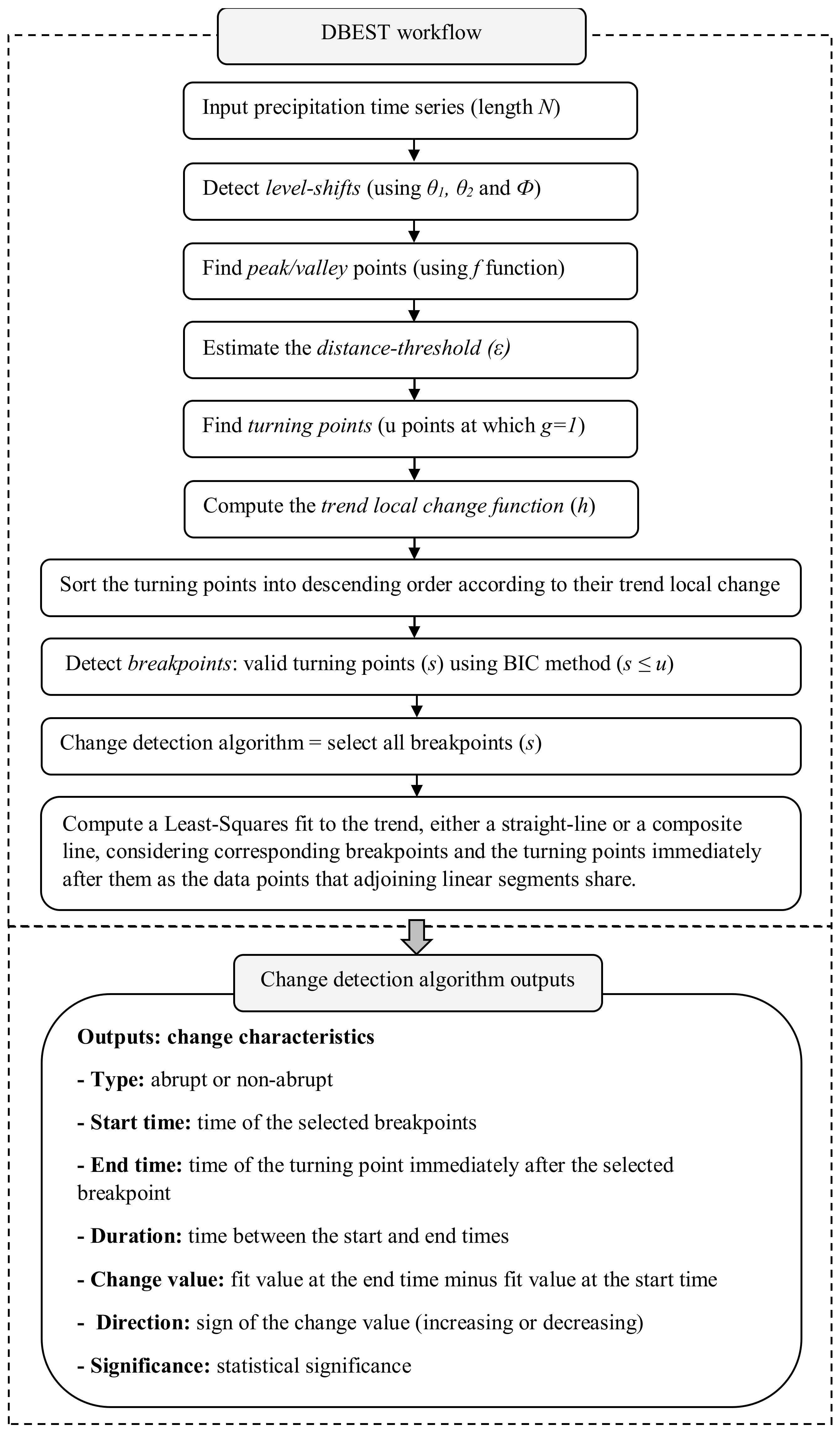
Figure 1. Flowchart of DBEST algorithm for detecting and characterizing changes in pixel-based precipitation datasets (after Jamali et al. [25]).
Remotesensing 14 05433 g001
Figure 2. (a) Mean annual precipitation and (b) coefficient of variation (CV) between 1998 and 2019 in 3B43.
Remotesensing 14 05433 g002
Figure 3. Abrupt and non-abrupt changes in the global precipitation time series, 1998–2019.
Remotesensing 14 05433 g003
Figure 4. An example of a typical (a) non-abrupt breakpoint with a three-year change duration and −180 mm change magnitude and (b) abrupt breakpoint with a one-year change duration and +247 mm change magnitude in the global precipitation time series.
Remotesensing 14 05433 g004
Figure 5. Start time of the breakpoints in the pixel-based global precipitation time series (1998–2019).
Remotesensing 14 05433 g005
Figure 6. Duration (year) of the abrupt and non-abrupt changes in the global precipitation time series (1998–2019).
Remotesensing 14 05433 g006
Figure 7. The magnitude of abrupt and non-abrupt changes in the global precipitation time series (1998–2019).
Remotesensing 14 05433 g007
Figure 8. (a) Distribution of all significant breakpoints (column) and abrupt and non-abrupt changes (lines) over different continents and (b) distribution of all significant breakpoints over the 1998–2019 period.
Remotesensing 14 05433 g008
Figure 9. (a) Distribution of all significant breakpoints (column) and abrupt and non-abrupt changes (lines) in different climate zones and (b) distribution of all significant breakpoints over the 1988–2019 period.
Remotesensing 14 05433 g009
Figure 10. (a) Abrupt and non-abrupt changes at 0.05% significance level and (b) their start time, in different climate zones over the 1998–2019 period.
Remotesensing 14 05433 g010
Table 1. User-defined thresholds in the DBEST’s change detection algorithm [Adapted from [25]].
ThresholdDescription
First level-shift-threshold (θ1)The lowest absolute difference in input data (precipitation) between the level-shift point and next datapoint
Duration-threshold (ϕ)The lowest period (time steps) within which the shift in the mean of the data level, before and after the level-shift point, persists, and the lowest spacing (time steps) between successive level-shift points.
Second level-shift-threshold (θ2)The lowest absolute difference in the means of the data calculated over period ϕ before and after the level-shift point
Change number (m)Number of greatest breakpoints of interest for detection
Statistical significance level (α)The statistical significance level used for testing the significance of detected changes
Table 2. Percentage of significant positive (Pos.) and negative (Neg.) breakpoints of precipitation on different continents.
Continent AsiaAfrica Europe N. AmericaS. AmericaAustraliaOceania
YearNeg.Pos.Neg.Pos.Neg.Pos.Neg.Pos.Neg.Pos.Neg.Pos.Neg.Pos.
19987.10.83.52.50.01.120.50.26.05.10.12.013.89.2
19991.31.16.21.71.60.40.60.22.41.51.82.34.63.1
20000.93.41.81.10.42.60.91.64.01.38.90.013.80.0
20010.45.31.33.38.13.22.62.52.70.818.50.00.00.0
20021.35.31.22.89.80.70.63.54.81.70.00.30.00.0
20034.20.31.65.20.05.10.17.10.41.90.00.10.01.5
20041.72.72.34.53.00.02.92.60.40.40.40.06.20.0
20052.81.32.13.21.26.07.42.00.23.51.33.60.01.5
20060.91.74.30.80.70.01.85.12.20.41.31.31.50.0
20072.31.03.33.90.00.21.21.81.71.80.11.20.00.0
20081.44.13.42.40.01.81.90.45.61.20.00.53.10.0
20091.24.52.81.60.50.91.93.18.18.40.137.40.01.5
20102.51.53.22.430.40.03.21.90.42.51.62.99.21.5
20110.83.01.14.70.43.35.81.04.61.611.10.015.40.0
20122.43.43.80.71.81.61.35.03.01.30.60.11.50.0
20132.73.21.32.60.20.20.12.31.92.30.01.31.50.0
20140.93.54.43.01.60.20.22.24.11.40.00.03.11.5
20151.82.91.70.70.04.20.80.71.33.10.00.00.00.0
20165.10.60.51.32.30.01.90.30.43.30.70.10.03.1
20170.38.80.21.70.07.00.40.31.20.80.40.00.03.1
Total41.758.350.050.061.838.256.243.855.544.546.953.173.826.2
Average2.12.92.52.53.11.92.82.22.82.22.32.73.71.3
Table 3. Percentage of significant positive (Pos.) and negative (Neg.) breakpoints in precipitation for different climate zones.
ClimateArid (%)Equatorial (%)Polar (%)Snow (%)Warm Temperate (%)
YearNeg.Pos.Neg.Pos.Neg.Pos.Neg.Pos.Neg.Pos.
19985.91.51.66.03.61.818.10.57.80.8
19993.51.52.51.42.10.61.70.22.41.0
20001.61.94.70.92.30.92.22.22.43.8
20012.13.63.01.40.92.24.35.62.23.8
20021.03.52.02.73.54.81.43.25.53.7
20032.83.30.51.20.80.41.32.00.92.6
20041.93.51.01.90.32.41.72.83.30.2
20052.71.90.86.57.71.02.21.02.82.7
20062.71.11.10.90.84.31.03.61.72.5
20072.42.44.41.62.12.90.61.81.01.1
20082.02.73.90.83.93.10.73.64.73.8
20091.95.56.410.51.65.41.31.21.24.6
20102.61.81.92.94.22.43.32.38.42.3
20111.93.44.41.82.81.13.92.31.92.2
20122.72.41.80.72.40.91.74.83.50.7
20131.63.02.80.64.32.62.02.30.71.5
20142.43.53.21.15.31.80.30.80.70.6
20151.61.71.35.43.84.30.41.31.11.5
20162.40.70.22.81.51.57.50.52.21.4
20170.35.10.60.91.00.60.33.20.54.4
Total46.054.048.151.954.945.155.444.755.045.1
Average2.32.72.42.62.72.32.82.22.72.3
Table 4. Statistical description of precipitation changes in different climate zones.
ClimateAridEquatorialPolarSnowWarm Temperate
Change (mm)Pos.Neg.Pos.Neg.Pos.Neg.Pos.Neg.Pos.Neg.
Mean164.0−174.3874.4−846.8194.2−159.5326.4−323.7574.5−634.3
Max2719.6−2.93122.1−223.01074.2−57.4981.9−98.64967.6−126.9
Min3.2−2113.6198.0−2998.457.7−1348.088.9−1547.0116.5−2801.8
Publisher’s Note: MDPI stays neutral with regard to jurisdictional claims in published maps and institutional affiliations.