Analysis of Diurnal Evolution of Cloud Properties and Convection Tracking over the South China Coastal Area

Abstract

Different diurnal rainfall cycles occur over the offshore and inland regions of the South China coastal area (SCCA). Inspired by these findings, in this study, we investigated the diurnal evolution features of cloud systems and cloud properties inside such systems for both the SCCA offshore and inland regions, using cloud data retrieved from a recently developed deep neural network model. Rainy day data for June 2017 revealed that the ice cloud optical thickness and top height reached their peak intensities at noon (~12 local standard time (LST)) over the offshore region, approximately 2 h later than the rainfall peak. Over the inland region, cloud and rainfall peaks simultaneously appeared from ~18 to 20 LST. When further examining the cloud-amount variation of different ice-cloud types, we found a clear diurnal oscillation in the medium-thick cloud amount over the offshore region, while for the inland region, this cloud type had no obvious diurnal peak, showing a low cloud amount throughout the day. This phenomenon suggests different inner structures and intensities between offshore and inland convections. To better elucidate the convection features over different regions, a tracking algorithm was applied to obtain various parameters, such as size, number, and duration of mesoscale convective systems. The strongest convections, which lasted over 12 h, tended to be abundant over the offshore region from ~03 to 12 LST, and an inland to offshore migration at ~03 LST was facilitated by the beneficial meteorological conditions observed at 113–116˚E, 20.5–22.5˚N.

1. Introduction

The South China coastal area (SCCA) receives most of its annual rainfall during the Mei-yu season (May–June). SCCA rainfall exhibits clear but different diurnal cycles for offshore and inland regions ([1,2]). Specifically, a narrow rainfall peak appears in the afternoon over the inland region, whereas the rainfall maximum appears in the morning over the offshore coast. The mechanisms governing diurnal cycles are complex and determined by processes that cross multiple scales. On a large scale, the Mei-yu season overlaps with the early phase of the East Asian summer monsoon, whereas at the synoptic scale, these diurnal precipitation cycles are controlled by local land–sea circulation ([3]).

Ref [4] (hereafter C19) investigated the modulatory effects of boreal summer intraseasonal oscillations on the SCCA rainfall diurnal cycle from a climatological-mean perspective. The rainfall pattern of offshore and inland regions is shown in Figures 1 and 3 in their study, respectively, while the different diurnal cycles are attributed to the land–sea breeze (Figure 2 of C19). Rainfall is generated from convective systems, essentially composed of clouds with different properties ([5]). In this paper, based on the rainfall diurnal cycles revealed by previous studies, we further raise the following questions: What are the cloud diurnal evolutions? Will there be any differences between the rainfall and the cloud diurnal features? In particular, we seek to answer these questions by taking into account the difference between the SCCA offshore and inland regions, so that the cloud systems and their relationships with the rainfall can be better understood and modeled in the future.

The absence of high-quality cloud property data has long been an obstacle to investigating mesoscale cloud variations. Cloud data should be available at a high spatiotemporal resolution for both day and night (24 h each day). Cloud properties retrieved from the solar band are only available during the daytime, whereas traditional physics-based algorithms, which use infrared measurements as input, cannot estimate a cloud optical thickness (COT) larger than ~10, owing to the limitation of the blackbody principle. Recently, ref [6] developed an image-based deep neural network model (DNN) for cloud property retrieval and used the brightness temperature of four Himawari-8 infrared bands as input. The performance of the DNN was then validated by active remote sensing from CloudSat, Cloud-Aerosol Lidar, and Infrared Pathfinder Satellite Observation (CALIPSO) ([7,8]) and was considerably superior to those of physics-based algorithms and pixel-by-pixel retrieval models. In this study, the DNN-retrieved cloud properties, such as the ice COT (ICOT), ice cloud top height (ICTH), and cloud amount, were used for diurnal analysis of the SCCA.

In addition, to obtain information on the separated convective system, we applied a convection tracking algorithm called sparse analysis for shape tracking (SAST), recently developed by [9] Compared with traditional tracking algorithms that set thresholds using the minimum brightness temperature and radius to identify convection, SAST utilizes pixel intensities of the input image and tracks their variation over time. SAST then decomposes each convection into several Gaussian ellipsoids, which enables the target convection to be deformable throughout its evolution so that the splitting and merging processes can be recorded, and a high accuracy can be ultimately ensured. In addition, the required convection parameters, such as size, number, and duration, of the mesoscale convective systems (MCSs) can be directly obtained as the algorithm output. These parameters will be further used to elucidate the different characteristics of offshore and inland convection over the SCCA.

This paper is structured as follows: Section 2 documents the data and method used in this study; Section 3 focuses on the diurnal characteristics of cloud properties and the attendant tracking results of cloud systems with SAST, in Section 3.3 we also explores the diurnal patterns of the meteorological fields; Section 4 presents the conclusions.

2. Data and Method

2.1. Precipitation Data

Precipitation data were obtained from Integrated Multi-satellite Retrievals for the Global Precipitation Measurement (GPM) mission (IMERG, [10]), which provides precipitation estimates every 30 min at a 0.1° × 0.1° spatial resolution over most of Earth’s surface. The latest version of the IMERG release includes precipitation estimates collected from 2000 to 2015 based on TRMM satellite observations and the more recent collection from the GPM satellite (2014–present). Here, we chose May and June (Mei-yu season of SCCA) from 2015 to 2018 to first check the precipitation intensity and continuity for different years in the area of interest.

The time series of different years’ mean precipitation (from 2015 to 2018) are shown for the offshore, inland, and whole SCCA with different colors in Figure S1. The occurrence and duration time of strong and continuous rainfall events varied from year to year. In 2015, the Mei-yu phenomenon appeared mainly in May, whereas in 2016 and 2017, primary rainfall events were observed in June. Their intensities were also observed to be different, especially when looking at both inland and offshore regions. Comparisons revealed that in 2017, the Mei-yu season rainfall in both offshore and inland regions was persistently high and had obvious diurnal features, which is why this year was selected for the current case study.

Based on a review of the daily mean rainfall pattern in June 2017 (Figure 1), only the rainy days (2, 3, and 11–21 of June 2017) that exhibited significant diurnal oscillations were selected for later analysis. Using data from these selected days, we reproduced the diurnal rainfall patterns for the offshore and inland regions of SCCA, as presented in C19, shown in Section 3.1. The current choice of 12-day data ensures that the objective of this study can be realized and saves computational cost, although to be technically accurate, the results in this study are safely repeatable on days in which both the offshore and inland regions have clear diurnal features in the SCCA during the Mei-yu season.

2.2. Cloud Property Retrieval Using the DNN Model

The cloud properties used in the analysis, including ICTH, ICOT, and cloud mask, were retrieved using the DNN model ([6]) developed for rapid and accurate cloud retrieval from Himawari-8 infrared measurements throughout the day (24 h/day). In addition to using the brightness temperature of the four infrared bands, we also used complementary variables such as the temperature profile and observation angles, as input data for the DNN model. Information on all input variables can be found in the paper by [6]. The retrieved cloud properties were available at a resolution of 0.02° at the nadir point and a timestep of 10 min, consistent with the original Himawari-8 standard data. Notably, the cloud mask of the DNN output was formatted as flags on each pixel that indicated clear sky, water cloud, and ice-cloud pixels. When computing the cloud amount, as shown in Section 3, the number of pixels of each cloud type was first counted and then averaged to obtain a daily or hourly mean pattern.

2.3. SAST Algorithm for MCS Tracking

In detail in Section 3.3, we applied a convective system tracking algorithm to separate the observed cloud systems into individual MCSs and to obtain the parameters of each MCS; differences between MCSs over inland and offshore regions can be thoroughly analyzed by considering their location, size, and duration. Previous studies have contributed to the tracking of MCSs using infrared satellite images and have applied the area-overlapping method ([11]) and region growing techniques, such as tracking of an organized convection algorithm through 3D segmentation (TOOCAN, [12]). Later, researchers used a set of thresholds, including the minimum brightness temperature and radius, to identify and track MCSs. However, these processes rely on pixel-based information and do not allow for splitting and merging, which may result in large multicenter MCSs being misrepresented as several smaller systems. The Kalman filter has also been applied to MCS tracking in recent years ([4,13]), although this process requires sampling of the parameters of each tracking object and assumes a normal distribution of movements, which limits accuracy.

The SAST algorithm used in this study is based on an off-the-grid sparse analysis algorithm. As a sparse-recovery theory in nature, SAST was designed to track deformable shapes (MCSs in the current context) and successfully overcome the issue of discretization. SAST decomposes each MCS into a set of 2D ellipsoid Gaussians (see Figure 3 in the paper by [9] for a better understanding) and tracks them continuously by flexibly recording the merging and splitting processes. For each frame, useful parameters, such as the shape and size of the MCS, can be directly obtained. When developing the SAST algorithm, [9] used brightness temperature as input for convective system identification, while, in this study, we utilized ICOT as input for the SAST to further improve its accuracy, as suggested by a previous work ([14]); note that only ICOTs of high clouds (ICTH ≥ 7 km) were used here.

Different definitions of MCS based on size and duration have been applied. For instance, [4] included only convective systems with a maximum area (brightness temperature lower than 235 K) larger than 10,000 km² and a duration over 3 h in the MCS pool. [15] further considered the precipitation area based on a major axis length greater than 100 km and set the minimum duration to 4 h. In this study, we set the threshold as a pixel number ≥ 2000, which yielded an equivalent radius ≥ 50 km for MCS selection. This threshold is based on empirical experience obtained when testing the SAST algorithm and has been shown to be the best option for cases over the SCCA during the Mei-yu season.

3. Results

3.1. Reproduction of Diurnal Rainfall Pattern

An interesting finding of C19 is that the offshore and inland regions of the SCCA have different diurnal rainfall features during the Mei-yu season, mainly manifested in their peak times. Upon analyzing the near-surface perturbation wind and temperature, they attributed this phenomenon to the land–sea breeze mechanism, as shown in Figure 2 of C19. The land breeze, which develops from evening to morning, leads to the morning peak in offshore rainfall, while the sea breeze, which develops from morning to afternoon, accounts for the maximum afternoon rainfall over the inland region. It is known that the rainfall is originated from convective systems, which are essentially formed by clouds with various properties. Therefore, based on C19, we further hypothesized that convective systems and the associated cloud properties would also have different evolution features over the offshore and inland regions of the SCCA.

The diurnal rainfall patterns shown in C19 were based on Mei-yu season rainfall data collected over 20 years for the SCCA. Here, to start the cloud investigation, we first reproduced the main pattern of these diurnal rainfalls with 12 days of IMERG data selected from June 2017. Figure 2 shows the spatial distribution of our reproduced diurnal rainfall patterns. Similar to C19, we defined the SCCA as the area denoted by the black box in Figure 2 of this study.

Figure 3 of C19 shows that the offshore maximum rainfall appears from 06 to 12 local standard time (LST), and the inland rainfall increases from ~15 to 18 LST. Compared with their results, the peak time of inland rainfall in our study showed a slight lag (~3 h) within the acceptable range when considering the difference between the utilized datasets and the chosen periods. A further comparison of the quantitative results between Figure 3 in this study and Figure 1 of C19 confirmed that the offshore rainfall peak time was from ~8 to 10 LST, whereas the inland rainfall peak occurred from ~16 to 20 LST. After obtaining the above reproduced results, we applied the selected days in a cloud analysis to determine the similarities or differences in the rainfall and cloud evolution features for the SCCA offshore and inland regions.

3.2. Diurnal Evolution of Cloud Properties

As in the rainfall analysis, we further checked the daily evolution patterns of cloud properties, such as ICOT, which is geographically presented in Figure 4, and ICTH, which is illustrated in Figure 5. As shown by [6], high clouds (>~7 km) are mainly composed of ice clouds, whereas low clouds below ~2 km are mainly composed of water clouds. To better investigate the cloud features inside the convective system, the variation of which mainly manifests on the high clouds, we used only ice clouds for analysis. In Figure 4 and Figure 5, for both ICOT and ICTH, clear but different diurnal evolutions can be observed for the offshore and inland regions. These panels show that cloud properties over the offshore region began to intensify in the morning (after ~06 LST) and reached peaks near 12 LST. Moreover, the inland ICOT and ICTH increased slightly from ~18 LST and reached a narrow peak from 21 to 00 LST. Then, the inland cloud systems gradually lost their intensities after ~03 LST, when offshore cloud systems began to establish.

Although the cloud evolution patterns differed between the offshore and inland regions of the SCCA, the ICOT and ICTH peak times were almost synchronous, with both appearing ~2 h later than the rainfall peak, especially over the offshore region. This feature was further supported by the quantitative results presented in Figure 6. The ICOT and ICTH over the offshore region began to grow at ~08 LST and reached their maximum intensities at around noon (~12 LST). Moreover, inland ICTH and ICOT peaks simultaneously appeared in the late afternoon from 18 to 20 LST.

A comparison with the results shown in Figure 3 clearly showed that for the SCCA offshore region, the ICOT and ICTH peaks appeared ~2 h later than the rainfall peak, which occurred at 10 LST. For the inland region, the cloud properties and rainfall approached maximum values almost simultaneously, although a slight 1 h discrepancy may have occurred because the inland rainfall peak started at ~17 LST. The different time lags between the cloud properties and rainfall peaks further revealed different convection structures or types in these two regions. For the offshore region, when the rainfall peaked, the cloud properties continued to increase in intensity. Two hours later, when the convection reached a maximum at the top height and cloud optical depth inside, the rainfall decreased significantly. However, over the inland region, the rainfall and cloud intensities peaked simultaneously, suggesting a different rainfall evolution mechanism corresponding to the cloud composition inside the convection.

To obtain additional details on the cloud systems, the ice clouds were further divided into three types, namely, thin, medium-thick, and thick, according to their ICOT values with thresholds of τ = 3 and τ = 20; thus, the evolution features, particularly the amount variation in the different cloud categories, could be captured. Figure 7 shows the quantitative results of cloud amount for the four cloud types, including ice clouds and water clouds, for the offshore and inland regions. As explained above, water clouds are mainly located below ~2 km and do not play an important role in convection formation or composition, as demonstrated by the gray line in Figure 7. Notably, the commonly used International Satellite Cloud Climatology Project (ISCCP) criterion for cloud classification was not applied to ice clouds here, because the ISCCP values are more suitable for all-cloud-included conditions; however, we only focused on the upper part of clouds in this study.

When referring to the rainfall pattern (Figure 3) in which the offshore rainfall peak appeared at 10 LST and the inland rainfall peaked from 17 to 20 LST, the pattern corresponded to different cloud stages. For example, in the offshore region, when the rainfall peaked (10 LST), the amount of thick clouds increased, and the amount of thin clouds was much higher than that of thick clouds. For the inland region, when the rainfall peaked (17 to 20 LST), thick clouds also presented a peak amount, which was similar to that of the thin clouds. Therefore, offshore convection appeared to have a larger anvil component, which was mainly composed of thin clouds.

Figure 8 shows the spatial distribution of cloud amount for the three ice cloud types, with 3 h as an interval. Thin ice clouds, with ICOT ≤ 3, exhibited a large amount over the offshore SCCA from ~20 to 09 LST and were abundant over the inland region from 03 to ~15 LST, which corresponded to the dissipation/re-establishment stage of convection. Obviously, offshore thin clouds appeared more frequently within a continuous area with a large size, whereas inland thin clouds were sparsely distributed over a smaller area.

The spatial distribution of medium-thick clouds (3 < ICOT ≤ 20) is presented in Figure 8i–p, and it elucidates the difference between the offshore and inland medium-thick cloud features observed in Figure 7. The offshore medium-thick cloud amount increased from ~15 LST, peaked from 18 to 21 LST, and decreased after ~00 LST, with evident diurnal variation. For the inland region, the overall amount showed no clear variation throughout the day, and no peak was observed. This phenomenon implies that medium-thick clouds are not a main component of inland convective systems, and the inner structure clearly differs relative to the offshore counterparts. Thick clouds (ICOT > 20; Figure 8q–x) are the most representative of the mature stage of cloud systems, and both the offshore and inland regions had apparent daily evolution patterns in these clouds. In addition, from ~09 to 19 LST, offshore propagation was observed, which may have been caused by the land–sea breeze and the inertia-gravity wave ([16]). In particular, a migration of convection appeared to occur from the inland-to-offshore areas at ~03 LST.

3.3. MCS Tracking Using the SAST Algorithm

The above analysis of cloud properties was next performed for the entire SCCA area; however, we could not separate the properties according to the different MCS series. To obtain the characteristics of each MCS, the SAST algorithm was applied for convection tracking and parameter extraction to better distinguish the features of offshore and inland MCSs. A case is displayed in Figure 9 to demonstrate the operation of the SAST algorithm. The first row shows the precipitation pattern on 16 June 2017, from 04 to 22 LST, and reveals that it gradually propagated from the inland to the offshore region, and the second row shows the ICOT pattern in each corresponding frame. The rainfall pattern was generally consistent with the cloud system, although a slight location difference may have occurred because of the time lag between development stages (see Section 3.2). When using the ICOT images as the input, the SAST output could be obtained, as shown in the third row of Figure 9. The identified MCSs are denoted by different colors, and the MCS centers, illustrated by red stars, were computed as the weighted centroid. Small individual systems composed of less than 2000 pixels were not counted as MCSs.

In addition to the identified MCSs and their central locations, the main morphological parameters, such as the MCS number and size (Figure 10), were obtained from the SAST output for the offshore and inland regions. The size of each MCS in each frame was computed as the number of pixels (N) inside, and the equivalent radius (R) was further derived using the following equation:

$$\pi R^2=N\times \left(9 {\mathrm{km}}^2\right)$$

(1)

The spatial resolution of Himawari-8 is ~0.02° (~2 km) at the nadir point, and when moving poleward, the resolution gradually decreases along with a reduction in the observing angles. For the SCCA area of interest, the size of each pixel was equivalent to approximately 9 km². When summing up the area of the pixels and approximating the MCS as a circle, the radius R can be obtained as shown in Equation (1).

The daily mean variation in MCS number and evolution pattern of MCS size for the offshore and inland regions are shown in Figure 10a,b, respectively. The peaks of MCS number and size were nearly consistent for the inland region and occurred from 18 to 20 LST. This peak time was also consistent with those for the inland ICOT and ICTH peaks, as shown in Figure 6. This consistency suggests that the convection intensity, cloud properties inside, and convection size develop synchronously over the inland area and are primarily favored by environmental variations during the afternoon.

For the offshore counterpart, the MCS size reached an obvious peak in the morning from 08 to 10 LST, and the MCS number increased and reached a maximum ~4 h later at ~13 LST, similar to the observed peak of cloud properties, which appeared at noon (12 LST). The inconsistency between the development of size and intensity suggests a more complex evolutionary mechanism for offshore MCSs. The large MCSs may split into smaller individual systems after the mean MCS size reaches a maximum, or a greater number of small MCSs may be formed, thereby increasing the MCS number. In addition, differences in the inner structures of the inland and offshore MCSs (Figure 7 and Figure 8) could also be confirmed. The minimum offshore MCS size was much smaller than that of its inland counterpart (Figure 10b), suggesting a larger oscillation amplitude of the offshore MCS size, the variation of which is more typical of deep convections that have clear diurnal intensity evolutions.

Because the time when MCSs appear in abundance is well identified, we further illustrated their distribution on a map for different hours of the day. In Figure 11, the MCSs are classified into four types according to their duration, which is used as an approximation of the intensity. MCSs lasting less than 6 and 9 h are illustrated with yellow and green dots, respectively, and tended to be sparsely distributed along the coastline. Medium-intensity MCSs lasting between 9 and 12 h are denoted by blue dots and were more frequently observed over the inland region. In addition to being attributable to the solar heating effect, these medium-intensity MCSs may be caused by land–sea breeze, as proposed by [17,18]. In addition, coastal mountains may strengthen inland convection by deepening the landward wind ([19]). The strongest MCSs lasting more than 12 h (denoted by red dots) were abundant over the inland coast from 18 to 03 LST and concentrated over the offshore coast from 03 LST to the following noon (12 LST). However, they were sparsely distributed along the coastline and showed no clear concentration.

Furthermore, for strong MCSs with a duration over 12 h, the starting and ending points are marked by purple and gray triangles in Figure 11, respectively. Ending points primarily appeared on panels 21–24 LST and 15–18 LST, whereas several starting points (marked with purple crosses) were found on the 03–06 LST panel over the offshore coast. In that specific panel, two ending points appeared over the inland region, indicating the disappearance of two convective events and the possible start of events over other regions. When further compared with the previous framework from 00 to 03 LST, where the MCSs were concentrated over the inland region and no starting or ending points were observed over SCCA (black box), an MCS migration from inland to offshore was found to occur at ~03 LST. This migration may have been caused or facilitated by the background environment during a specific period. Subsequently (as described in the next section), we examined the meteorological conditions to obtain additional details and identify possible causal factors.

3.4. Meteorological Fields

On a large scale, the South China Sea during the Mei-yu season is dominated by the southwest monsoon, which transports moisture from the tropical ocean to subtropical continents. This circulation could enhance the convective instability over southern Asia but has relatively slow temporal variations (i.e., on a seasonal scale). Moreover, synoptical-scale disturbances, such as the land–sea breeze, have been revealed as a key factor driving meteorological variations over the SCCA ([20,21]). Here, we first examined the diurnal pattern of wind and velocity anomalies at 850 hPa based on hourly data from the European Center for Medium-Range Weather Forecasts (ECMWF) fifth-generation reanalysis product ERA5 ([22]), as shown in Figure 12.

In the early morning (from ~03 LST), large positive vertical velocity anomalies appear over the continental area and adjacent sea of the SCCA. Meanwhile, the beneficial northward wind brings a larger amount of humidity from the open sea. This favorable condition lasts from 03 to 06 LST, which greatly facilitates the initiation and development of strong offshore convections, as shown in Figure 11. Upon the establishment of a beneficial environment (moisture and vertical velocity) over the offshore coastal area, convections are more likely to migrate inland over a longer duration. In contrast, inland convection does not seem to be determined by meteorological changes. During the establishment period from 09 to 18 LST, a slight increase was observed in the inland vertical velocity; moreover, the driving force underlying inland convection development may have been other factors such as the solar heating effect and local orography.

In addition to the wind field, the vertical moist stability (VMS, [23]), which is similar to the equivalent potential temperature, was investigated to determine the diurnal evolution of convective instability over the study domain. First, the moist static energy (MSE) was computed using Equation (2):

$$MSE=C_{p}T+gz+L_{v}q$$

(2)

where $C_p$ is the specific heat at constant pressure, T is the absolute temperature, g is the gravitational acceleration, z is the height above the surface, $L_v$ represents the latent heat of vaporization, and q is the specific humidity. Then, the VMS was derived as the difference in MSE between the middle (400–700 hPa) and lower (700–1000 hPa) atmospheres, as follows:

$$VMS=MS{E}_{⟨400–700\mathrm{hPa}⟩}-MS{E}_{⟨700–1000\mathrm{hPa}⟩}$$

(3)

As suggested previously ([24,25]), obtaining the change patterns of diagnostic fields, such as vertical velocity and static stability, will help provide a better understanding of how the environment in which clouds form and vary has been modified by the circulation and meteorological fields. The inland unstable energy increased from ~15 LST (Figure 13), which was nearly 3 h ahead of the intensity peak of inland cloud properties and serves as a thermodynamic requirement for cloud evolution. The inland instability decayed afterward, and the offshore instability increased from 00 LST and gradually decayed after 06 LST, when the offshore convections had developed to the mature stage. At ~00 LST, a connection between the inland and offshore VMS and a subsequent splitting occurred, as shown in Figure 13h. This spatial pattern of convective instability further supports the migration or initiation of strong MCSs over the offshore region at ~03 LST.

4. Conclusions

In this study, we investigated the diurnal features of cloud systems and cloud properties during the rainy days of June 2017 in the Mei-yu season for the SCCA. Based on the previously revealed differences in rainfall diurnal cycles of the SCCA offshore and inland regions, we further focused on the diurnal evolution features of clouds over these two areas by applying the cloud properties retrieved using the most recently developed DNN model and the SAST image-based convection tracking algorithm. The diurnal precipitation patterns were first reproduced as shown in Figure 1 and Figure 3 in the paper by C19 using IMERG data, and the hourly meteorological fields from ERA-5 were analyzed to elucidate the underlying mechanism. The principal findings of this study are summarized as follows:

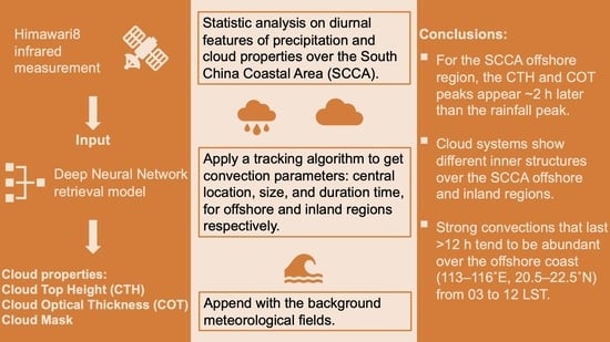
• Similar to the precipitation evolution, ICOT and ICTH showed different diurnal cycles and peak times over the offshore and inland regions. Additionally, a time lag occurred between the rainfall and cloud peaks. Specifically, the offshore ICOT and ICTH reached peak intensities at ~12 LST, which was 2 h after the rainfall peak (~10 LST). Moreover, over the inland region, rainfall and cloud peaks appeared synchronously at ~18–20 LST. This difference in synchronism between the offshore and inland regions suggests that the convection types and internal evolving mechanisms are different over these two regions.
• Upon investigating the diurnal cloud amount evolution of different ice cloud types (Figure 7), over the offshore region, thick clouds were found to approach the maximum amount first, medium-thick clouds reached a peak amount several hours later, and the thin cloud amount eventually increased during the dissipation or re-establishment stages. This process is typical of the evolution of strong convection with a clear phase transition. However, within the inland MCSs, medium-thick clouds first peaked at ~16 LST, which was 3 h ahead of the thick cloud peak, and persisted at a high amount until ~02 LST. The rainfall peak also overlapped with the different cloud configurations in these two regions. These phenomena suggest different cloud structures and features within offshore and inland convections.
• SAST tracking of the daily MCS size and number evolution (Figure 10) also confirmed the different intensities of offshore and inland MCSs and showed that the offshore MCSs are more typical of strong convections that have an apparent diurnal cycle. Furthermore, examination of the spatiotemporal distribution of MCSs with different duration lengths showed that the medium-intensity MCS, which lasts for 9–12 h, is primarily located along the inland coastline, whereas the strong MCS, which lasts over 12 h, is primarily located over the offshore coast from 03 to 12 LST.
• The inland to offshore migration of MCSs was confirmed to occur at ~03 LST (Figure 8 and Figure 11). This migration could be explained by the favorable meteorological environment formed during the same period. From 00 to 03 LST, obvious vertical velocity anomalies appeared over the offshore coast, and southeasterly winds introduced a large amount of moisture from the open sea. Both conditions facilitated the initiation and development of offshore convection at midnight. In addition, an inland to offshore migration of unstable energy was observed at ~00 LST (Figure 13), which serves as a beneficial thermodynamic condition for cloud formation afterward.

To better elucidate the mechanisms underlying offshore and inland convection evolution, especially for inland convection, which presents rainfall that appears to be less related to thick ice clouds, model simulations that focus on the SCCA orography effect are needed. As suggested by a previous work ([26]), coastal convections are frequently influenced by both the topographically generated circulations and diurnally forced circulations, the combination of which makes the coastal convections unique and complicated in mechanism. Therefore, future studies that take into account the topography effect over SCCA would further help to reveal the relationships between rainfall and clouds, as well as their evolution processes, on a diurnal scale. Here, we mainly presented an innovative framework, including the application of a newly developed cloud property retrieval model and a state-of-the-art convection tracking algorithm for studying the diurnal cloud evolution in the Mei-yu season over the SCCA. Although the obtained results hold for rainy days of June 2017, to obtain general conclusions, additional rainfall events over different years should be included for a comprehensive investigation, and we leave such extended work for future studies.

References

1. Chen, X.; Zhao, K.; Xue, M.; Zhou, B.; Huang, X.; Xu, W. Radar observed diurnal cycle and propagation of convection over the Pearl River delta during Mei-yu season. J. Geophys. Res. Atmos. 2015, 120, 12557–12575. [Google Scholar] [CrossRef] [Green Version]
2. Jiang, Z.; Zhang, D.-L.; Xia, R.; Qian, T. Diurnal variations of presummer rainfall over southern China. J. Clim. 2017, 30, 755–773. [Google Scholar] [CrossRef]
3. Chen, X.; Zhang, F.; Zhao, K. Diurnal variations of the land–sea breeze and its related precipitation over south China. J. Atmos. Sci. 2016, 73, 4793–4815. [Google Scholar] [CrossRef]
4. Chen, D.; Guo, J.; Yao, D.; Lin, Y.; Zhao, C.; Min, M.; Xu, H.; Liu, L.; Huang, X.; Chen, T.; et al. Mesoscale convective systems in the Asian monsoon region from Advanced Himawari Imager: Algorithms and preliminary results. J. Geophys. Res. Atmos. 2019, 124, 2210–2234. [Google Scholar] [CrossRef] [Green Version]
5. Wang, X.; Iwabuchi, H.; Takahashi, N. Characteristics of diurnal pulses observed in Typhoon Atsani using retrieved cloud property data. SOLA 2019, 15, 137–142. [Google Scholar] [CrossRef]
6. Wang, X.; Iwabuchi, H.; Yamashita, T. Cloud identification and property retrieval from Himawari-8 infrared measurements via a deep neural network. Remote Sens. Environ. 2022, 275, 113026. [Google Scholar] [CrossRef]
7. Delanoë, J.; Hogan, R.J. A variational scheme for retrieving ice cloud properties from combined radar, lidar, and infrared radiometer. J. Geophys. Res. Atmos. 2008, 113, D07204. [Google Scholar] [CrossRef] [Green Version]
8. Delanoë, J.; Hogan, R.J. Combined CloudSat-CALIPSO-MODIS retrievals of the properties of ice clouds. J. Geophys. Res. Atmos. 2010, 115, D00H29. [Google Scholar] [CrossRef] [Green Version]
9. Courbot, J.B.; Duval, V.; Legras, B. Sparse analysis for mesoscale convective systems tracking. Signal Processing Image Commun. 2020, 85, 115854. [Google Scholar] [CrossRef] [Green Version]
10. Huffman, G.; Bolvin, D.; Braithwaite, D.; Hsu, K.; Joyce, R.; Xie, P.; Yoo, S.H. Algorithm Theoretical Basis Document (ATBD) Version 4.5: NASA Global Precipitation Measurement (GPM) Integrated Multi-SatellitE Retrievals for GPM (IMERG); NASA: Greenbelt, MD, USA, 2018. [Google Scholar]
11. Mathon, V.; Laurent, H. Life cycle of Sahelian mesoscale convective cloud systems. Q. J. R. Meteorol. Soc. 2001, 127, 377–406. [Google Scholar] [CrossRef]
12. Fiolleau, T.; Roca, R. An algorithm for the detection and tracking of tropical mesoscale convective systems using infrared images from geostationary satellite. IEEE Trans. Geosci. Remote Sens. 2013, 51, 4302–4315. [Google Scholar] [CrossRef]
13. Huang, X.; Hu, C.; Huang, X.; Chu, Y.; Tseng, Y.h.; Zhang, G.J.; Lin, Y. A long-term tropical mesoscale convective systems dataset based on a novel objective automatic tracking algorithm. Clim. Dyn. 2018, 51, 3145–3159. [Google Scholar] [CrossRef] [Green Version]
14. Li, W.; Zhang, F.; Yu, Y.; Iwabuchi, H.; Shen, Z.; Wang, G.; Zhang, Y. The semi-diurnal cycle of deep convective systems over Eastern China and its surrounding seas in summer based on an automatic tracking algorithm. Clim. Dyn. 2021, 56, 357–379. [Google Scholar] [CrossRef]
15. Feng, Z.; Leung, L.R.; Liu, N.; Wang, J.; Houze, R.A., Jr.; Li, J.; Hardin, J.C.; Chen, D.; Guo, J. A global high-resolution mesoscale convective system database using satellite-derived cloud tops, surface precipitation, and tracking. J. Geophys. Res. Atmos. 2021, 126, e2020JD034202. [Google Scholar] [CrossRef]
16. Du, Y.; Rotunno, R. Diurnal cycle of rainfall and winds near the south coast of China. J. Atmos. Sci. 2018, 75, 2065–2082. [Google Scholar] [CrossRef]
17. Huang, W.-R.; Chang, Y.-H.; Hsu, H.-H.; Cheng, C.-T.; Tu, C.-Y. Summer convective afternoon rainfall simulation and projection using WRF driven by global climate model. Part II: Over South China and Luzon. Terr. Atmos. Ocean. Sci. 2016, 27, 673–685. [Google Scholar] [CrossRef] [Green Version]
18. Simpson, M.; Warrior, H.; Raman, S.; Aswathanarayana, P.; Mohanty, U.; Suresh, R. Sea-breeze-initiated rainfall over the east coast of India during the Indian southwest monsoon. Nat. Hazards 2007, 42, 401–413. [Google Scholar] [CrossRef] [Green Version]
19. Riley Dellaripa, E.; Maloney, E.; Toms, B.; Saleeby, S.; Van den Heever, S. Topographic effects on the Luzon diurnal cycle during the BSISO. J. Atmos. Sci. 2020, 77, 3–30. [Google Scholar] [CrossRef]
20. Huang, L.; Luo, Y.; Zhang, D.-L. The relationship between anomalous presummer extreme rainfall over south China and synoptic disturbances. J. Geophys. Res. 2018, 123, 3395–3413. [Google Scholar] [CrossRef] [Green Version]
21. Zhang, M.; Meng, Z. Impact of synoptic-scale factors on rainfall forecast in different stages of a persistent heavy rainfall event in south China. J. Geophys. Res. Atmos. 2018, 123, 3574–3593. [Google Scholar] [CrossRef]
22. Hersbach, H.; Bell, B.; Berrisford, P.; Hirahara, S.; Horányi, A.; Munoz-Sabater, J.; Nicolas, J.; Peubey, C.; Radu, R.; Schepers, D.; et al. The ERA5 global reanalysis. Q. J. R. Meteorol. Soc. 2020, 146, 1999–2049. [Google Scholar] [CrossRef]
23. Neelin, J.D.; Held, I.M. Modeling tropical convergence based on the moist static energy budget. Mon. Weather. Rev. 1987, 115, 3–12. [Google Scholar] [CrossRef]
24. Grise, K.M.; Medeiros, B. Understanding the varied influence of midlatitude jet position on clouds and cloud radiative effects in observations and global climate models. J. Clim. 2016, 29, 9005–9025. [Google Scholar] [CrossRef]
25. Li, Y.; Thompson, D.W.; Stephens, G.L.; Bony, S.A. Global survey of the instantaneous linkages between cloud vertical structure and large-scale climate. J. Geophys. Res. Atmos. 2014, 119, 3770–3792. [Google Scholar] [CrossRef]
26. Yu, C.K.; Lin, C.Y. Formation and maintenance of a long-lived Taiwan rainband during 1–3 March 2003. J. Atmos. Sci. 2017, 74, 1211–1232. [Google Scholar] [CrossRef]
Figure 1. Daily rainfall amount over the South China coastal area (SCCA, cyan bar), including offshore and inland regions, as denoted by red and blue markers, respectively.
Remotesensing 14 05039 g001
Figure 2. Three-hourly mean rainfall evolution (shown on the map) based on IMERG data. Days were selected from June 2017. The region highlighted with a black box is the SCCA, the area of focus in this study.
Remotesensing 14 05039 g002
Figure 3. Daily mean rainfall intensities are shown quantitatively for offshore and inland regions, based on Figure 2.
Remotesensing 14 05039 g003
Figure 4. Same as in Figure 2 but for mean ice cloud optical thickness (ICOT) retrieved using the deep neural network (DNN) model by [6], with Himawari-8 infrared measurement as input.
Remotesensing 14 05039 g004
Figure 5. Same as in Figure 2 but for mean ice cloud top height (ICTH) retrieved using the DNN model, with Himawari-8 infrared measurement as input.
Remotesensing 14 05039 g005
Figure 6. Quantitative demonstration of the results in Figure 4 and Figure 5 for the area-averaged (a) ICTH (km) and (b) ICOT. Results for the offshore and inland areas are denoted by red and blue lines, respectively.
Remotesensing 14 05039 g006
Figure 7. Daily mean evolution in the amount of four cloud types, with averaged values for the offshore and inland areas. The water cloud amount is plotted in gray, whereas ice clouds are decomposed into three cloud types, namely, thin, medium (medium-thick), and thick, according to their cloud optical thickness values.
Remotesensing 14 05039 g007
Figure 8. Daily mean cloud amount evolution over the SCCA within a 3 h interval. The first two rows (ah) present the thin ice clouds results, the next two rows (ip) show the medium-thick ice-cloud results, and the last two rows (qx) show the thick ice cloud results.
Remotesensing 14 05039 g008
Figure 9. One-day case (6 h intervals) showing the SAST tracking results on each input frame. The first row (ad) shows the precipitation patterns, the second row (eh) shows the ICOT images, and the last row (il) shows the MCSs tracked using the SAST method and ICOT images as input. The identified convection centers are denoted by red stars, and all times are consistent for each column among these three rows.
Remotesensing 14 05039 g009
Figure 10. Daily mean evolution of (a) the number and (b) size of mesoscale convective systems based on the SAST output over the SCCA offshore and inland regions, as denoted by red and blue markers, respectively.
Remotesensing 14 05039 g010
Figure 11. Identified MCSs are classified into four categories, as denoted by different markers, according to their duration. The points represent convection centers collected from each frame. For the strong convections that last over 12 h, their start and end points are further marked with a purple cross and gray triangle, respectively.
Remotesensing 14 05039 g011
Figure 12. Composited anomalies of vertical velocity (shaded) and horizontal wind arrows (m/s) at 850 hPa over the SCCA area. Hourly data are obtained from June 2017 and shown in the panels based on 3 h intervals. SCCA is not marked up in this figure, and the shown map scale is the same as before.
Remotesensing 14 05039 g012
Figure 13. Same as in Figure 12 but for the vertical moist stability anomaly.
Remotesensing 14 05039 g013
Publisher’s Note: MDPI stays neutral with regard to jurisdictional claims in published maps and institutional affiliations.