Abstract
Watershed modelling is crucial for understanding fluctuations in water balance and ensuring sustainable water management. The models’ strength and predictive ability are heavily reliant on inputs such as topography, land use, and climate. This study mainly focuses on quantifying the uncertainty associated with the input sources of the Digital Elevation Model (DEM), Land Use Land Cover (LULC), and precipitation using the Soil and Water Assessment Tool (SWAT) model. Basin-level modelling is being carried out to analyze the impact of source uncertainty in the prediction of streamflow. The sources for DEM used are National Elevation Dataset (NED)-United States Geological Survey (USGS), Shuttle Radar Topographic Mission (SRTM), and Advanced Spaceborne Thermal Emission and Reflection Radiometer (ASTER), whereas for LULC the sources were the National Land Cover Database (NLCD), Continuous Change Detection Classification (CCDC), and GAP/LANDFIRE National Terrestrial Ecosystems dataset. Observed monitoring stations (Gage), Climate Forecast System Reanalysis (CFSR), and Tropical Rainfall Measuring Mission (TRMM) satellites are the respective precipitation sources. The Nash-Sutcliffe Efficiency (NSE), Coefficient of Determination (R2), Percent Bias (PBIAS), and the ratio of Root Mean Square Error to the standard deviation (RSR) are used to assess the model’s predictive performance. The results indicated that TRMM yielded better performance compared to the CFSR dataset. The USGS DEM performs best in all four case studies with the NLCD and CCDC LULC for all precipitation datasets except Gage. Furthermore, the results show that using a DEM with an appropriate combination can improve the model’s prediction ability by simulating streamflows with lower uncertainties. TheVIKOR MCDM method is used to rank model combinations. It is observed from MCDM analysis that USGS DEM combinations with NLCD/CCDC LULC attained top priority with all precipitation datasets. Furthermore, the rankings obtained from VIKOR MCDM are in accordance with the validation analysis using SWAT.
1. Introduction
Climate change, population increase, and urbanization are the critical reasons for water stress worldwide. As a result, understanding and modelling hydrological processes becomes crucial for water resources planning, design, and management. One of the most practical solutions is to develop models (conceptual, empirical, and physically-based models) that can simulate hydrological processes, including the effects of variations in weather, soil properties, and land management practices. The conceptual models employ simple mathematical concepts to represent a system but ignore the spatial variability by lumping the entire watershed characteristics. On the other hand, empirical models are observation-oriented and transform rainfall into runoff without reference to the physical processes. These are also classified as black-box models since limited/no information about the system’s internal processes is known. Physical models consider the watershed’s spatial and temporal variations to mimic real-world processes accurately. These models can also integrate critical processes related to the atmosphere, geosphere, and biosphere. Due to its inherent advantages, physically-based models are considered the best alternative for decision-makers in integrated watershed management.
The Soil and Water Assessment Tool (SWAT) [1] is the most popular among the physically-based hydrological models due to its flexibility in solving water resources problems and the availability of open-source code [2]. It has wide applications in integrated watershed management, including prediction of streamflow/runoff, evapotranspiration, groundwater recharge, and sub-surface flow. It can simulate streamflows for a watershed spanning thousands of square kilometers. The model originated as a culmination of Chemicals, Runoff, and Erosion from Agricultural Management Systems (CREAMS) [3], Groundwater Loading Effects on Agricultural Management Systems (GLEAMS) [4], and Simulator for Water Resources in Rural Basins (SWRRB) [5]. It has undergone numerous reviews and capability expansions as part of the continual evaluation. Figure 1 depicts the salient features of the SWAT model and its notable advances up to SWAT 2012. Gassman et al. [2] found that the SWAT is a versatile and effective tool for simulating diverse watershed problems. Zuoda et al. [6] compared SWAT with the Generalized Watershed Loading Function (GWLF) model. The study showed that the SWAT is better suited for projects requiring higher accuracy and data-scarce basins. Moreover, the study also indicated that the concept of spatial variability does not exist in GWLF, unlike SWAT. Hence, the latter provides a precise description of the actual hydrological processes. Jaiswal et al. [7] compared the SWAT model with two conceptual models (TANK and the Australian Water Balance Model (AWBM)). They found that the SWAT model can identify the impact of LULC, weather, and managerial practices better than the other two conceptual models. Recently, Nasiri et al. [8] showed that the SWAT model can also be applied effectively in arid and semi-arid regions.
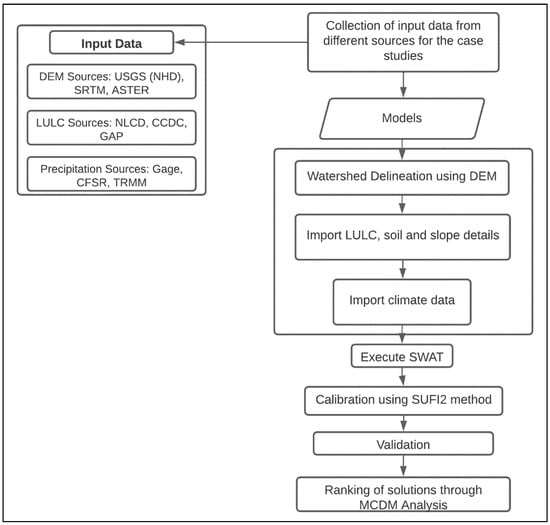
Figure 1.
Hydrological modelling framework used to carry out the uncertainty analysis in the prediction of streamflows.
The SWAT model requires several inputs related to watershed characteristics such as the Digital Elevation Model (DEM), Land Use Land Cover (LULC), soil data, and hydroclimatic factors (such as precipitation, temperature, wind speed, relative humidity, and solar radiation). These inputs are useful in modelling the complex rainfall-runoff processes and to assess the effect of various management activities such as sediment transport, water quality, and agriculture chemical yields. However, the number of inputs used in SWAT increases the uncertainty in streamflow prediction. The input uncertainties are classified into two categories: data sources and resolution of remote sensing data. It is to be noted that the various data sources (with the same resolution) use different algorithms, inherently making the data uncertain. For example, the different techniques to obtain the data sources include (i) DEM data: stereo optical imagery, laser altimetry (LiDAR), radar altimetry, and Interferometric Synthetic Aperture Radar (InSAR); (ii) LULCs data: CCDC and Terrestrial Ecological Systems Classification framework for LULCs; (iii) Precipitation data: Reanalysis and satellite.
Cotter et al. [9] noted that the resolution of the input DEM data had the most significant impact on the SWAT model output of the Moores Creek watershed in Arkansas, while land use and soil data resolutions had minimal effects on flow forecasts. According to Zhen et al. [10], quantifying uncertainty with the input factors of elevations and land cover change is necessary. It helps the modeler to evaluate the reliability of the models. Kumar et al. [11] concluded that the optimal DEM grid resolution for the specific watershed and output should be known to reduce uncertainty and suggested using a DEM of less than 300 m for flow, as the desired output was obtained with ±10% relative error. Fan et al. [12] demonstrate that land-use resolution affects the outcomes of model simulations. The quality of the DEM is less significant than the quality of the land use map in hydrological modelling. Furthermore, the study found no significant change in surface runoff estimates for DEM cell sizes below 100 m. Most of these studies have focused on input resolution uncertainty and showed the impact of DEM and LULC resolution on streamflow prediction. However, only limited studies are carried out on source uncertainty for DEM and LULCs. Gautam et al. [13], Munoth & Goyal [14], and Sukumaran & Sahoo [15] showed that the model performance is insensitive to variation in the DEM sources in streamflow prediction. Kamali et al. [16] investigated the effect of numerous LULC and climate data obtained from various sources and concluded that discharge prediction is less susceptible to different land use sources. Cuceloglu et al., [17] conducted a study with two different LULC datasets (Landsat satellite image and CORINE) and showed that the sources are less susceptible to streamflow prediction. Numerous studies have been carried out on precipitation sources [18,19,20,21]. Setti et al. [22] showed that the TRMM data performs better than CFSR in the streamflow prediction. Zhang et al., [21] showed that the TRMM data performs better than PERSSIAN- CDR for simulating hydrological processes such as streamflow, GW recharge, and evapotranspiration. Dutta et al. [23] conducted a study showing that the highest disagreement between the observed and predicted stream flows is for CFSR data.
A number of studies have quantified the uncertainties in the SWAT model with different calibration algorithms such as Generalized Maximum Likelihood Algorithm (GLUE) [24], Parameter solution (ParaSol) [25], and Sequential Uncertainty Fitting (SUFI2) [26]. Khoi et al. [27] identified the uncertainty in the SWAT model by employing the GLUE, Parasol, Particle Swarm Optimization (PSO), and SUFI2 algorithms using the SWAT CUP tool. The investigation revealed that due to the requirement of the lesser runs to achieve good prediction and model performance across all of the techniques, SUFI2 is the best technique. Chen et al. [28] performed a SWAT analysis on the Weijing River watershed in China with three calibration algorithms: GLUE, SUFI2, and Parasol. The results showed that due to its high accuracy (R2 and NSE), best measurement coverage (P-factor), and relatively low uncertainty effects (R-factor), SUFI2 might effectively capture modelling uncertainties and measure their consequences. Tang et al. [29] also performed the SWAT analysis with four algorithms:GLUE, SUFI2, PSO, and Parasol, and concluded that SUFI2 is a robust method for evaluating the model, parameter, and input uncertainties.
Most of the studies that quantified the uncertainties in the prediction of streamflows using SWAT is limited to (i) DEM and LULC resolution, (ii) the individual effect of DEM, LULC, and Precipitation sources, and (iii) calibration algorithms. However, the hydrological modelling processes are affected by topography, land use, and climate data (especially precipitation). Hence, it is necessary to quantify the input source uncertainties from the combined effects of different remote sensing data (DEM, LULC) and precipitation data sources for different topographic and climatic regions. Quantification will help the modelers to select the sources with the least uncertainty for optimal prediction of streamflows, which further reduces the risk and helps in the sustainable design and management of hydraulic structures, water distribution networks, irrigation supply, etc. The study yields various model combinations based on the different input sources. As it is complex and arduous to rank the combinations based on visual interpretation, the Multi-Criteria Decision Making (MCDM) method has been widely used in decision making. MCDM techniques have a broad implementation in water resource engineering in selecting the optimal solution based on different criteria. Mohammed et al. [30] used the MCDM method for prioritizing the potential impact of various pollution sources on surface and groundwater contamination. MCDM techniques have been employed to rank global climate models [31] and evapotranspiration models [32]. These studies suggest the effectiveness of MCDM methods as a support tool for decision-making in water resources management. Various MCDM methods have been developed to rank the solutions. Some of the significant MCDM methods are Technique for Order Preference by Similarity to an Ideal Solution (TOPSIS), Analytical Hierarchy Process (AHP), ELimination and (Et) Choice Translating Reality (ELECTRE), Vlse Kriterijumska Optimizacija I Kompromisno Resenje (VIKOR), and Preference Ranking Organization Method for Enrichment Evaluations (PROMTHEE). According to Chang and Yim [33], VIKOR is an essential tool for a robust decision-making framework under uncertainty. It provides a compromise solution by considering both the total and individual satisfaction of the alternative, thereby considering their relative importance. The method prioritized adaptation strategies under uncertain climate change scenarios [34]. Golfam et al. [35] ranked water-supply system simulations based on the VIKOR MCDM method. Bhattacharya et al. [36] demonstrated that the VIKOR model performs better than other MCDM techniques in prioritizing sub-basins for management activities. In this study, the VIKOR method is selected to rank the performance of the SWAT model combinations.
This study aims to help the modelers to select the best input source combination obtained from MCDM analysis for the watersheds with similar topographic and climatic backgrounds for the optimal prediction of streamflows, The prediction performance of the input sources is dependent on each other; hence, the use of inappropriate combinations of the sources will lead to the simulation of streamflows with higher uncertainty. The study aims to select the appropriate model combinations from the available input (DEM-LULC-Precipitation) datasets, despite the absence of higher priority input sources, for optimal streamflow prediction. Furthermore, the study will further help the decision-makers for efficient planning and management of water resources leading to the economical and sustainable growth of the nations.
Section 2 provides the study’s methodology and gives a brief framework for the research. Section 3 provides a detailed explanation of the case study selected for the analysis. Section 4 presents a detailed analysis of the results and discusses them in different subsections. Finally, the overall analysis conclusion is followed by references used in the study.
2. Materials and Methods
The proposed hydrological modelling framework for the uncertainty analysis in the prediction of streamflow is shown in Figure 1. The framework can be divided into the following three sections: (i) the SWAT model, (ii) Calibration analysis using SUFI2, and (iii) the MCDM approach.
2.1. SWAT Model
The SWAT model is an aggregated model that incorporates both surface and channel environmental processes. The model is widely available and allows hydrologists to simulate the quality and quantity of surface water worldwide [1]. The SWAT model is based on a continuous-time geographical distribution that examines the influence of management techniques on water and sediment yields in an ungauged basin capable of running for lengthy periods. SWAT can also be used to model an individual watershed or an entire network of watersheds that are connected hydrologically. Based on the slope, land use, management, and soil distributions, the watershed is divided into numerous sub-basins and smaller units called Hydrologic Response Units (HRUs). The HRU level analysis facilitates the identification of spatial scale variation of effects due to changes in watershed characteristics. The SWAT model sub-basins can be divided into different components such as hydrology, nutrients, sedimentation, weather, crop development, land management, and pesticides [37]. The study primarily focuses on the hydrologic component, mainly founded on the Water Mass Balance equation (Equation (1)).
where SWt is the overall humidity of soil at time t, which is expressed in days, Ri is rainfall volume measured from Precipitation in mm, SWo is initial humidity, Pi is the percolation of water seeping in from the soil, Qi is the volume of Surface Runoff, ETi is Evapotranspiration and QRi is groundwater runoff volume.
Runoff can be predicted using the curve number method (Equation (2)).
where, R = daily rainfall (mm); Q = runoff in mm; S = retention parameter; S can be calculated by the following SCS equation (Equation (3)).
CN2 is the Curve Number for normal antecedent moisture conditions (AMC II). The model provides three methods for calculating Evapotranspiration: the Penman-Monteith, Hargreaves, and Priestley-Taylor methods (Supplementary Material).
2.2. SUFI2 Calibration Model
The SUFI2 method is used for calibrating, validating, and analyzing the sensitivity and uncertainty of the output generated from the SWAT model. The uncertainty in the input parameters has been characterized as uniform probability distributions. In contrast, the uncertainty in simulation results is defined using the 95 percent prediction uncertainty of output variables acquired by Latin Hypercube Sampling (LHS), a technique used for producing random samples of parameter values. The sensitivity analysis identifies the critical parameters for the watersheds with the global sensitivity method and the One At a Time (OAT) method. In the global sensitivity analysis procedure, parameter sensitivities were described as a multiple regression system, which was then used to determine the statistical significance value of the parameter sensitivity. A t-test (Student’s t-distribution) was used, and the t-Stat, which means a parameter divided by its standard error, was used to evaluate parameter sensitivity. Another indicator used to assess uncertainty was the p-value, which measures the null hypothesis of the t-test, and which states that the coefficient has no effect (equal to zero). A parameter with a high t-Stat value and a low p-value is generally more sensitive [38]. The sensitive parameters were then used for the calibration, with 1000 simulations per iteration. The iterations were stopped when the objective function (NSE) reached a saturation level and should be more than the satisfactory value (NSE > 0.5). The P-factor and R-factor are two indicators that determine the model’s robustness and uncertainty. The P and R-factor are 100% and 0% in an ideal condition, respectively, when the simulation coincides with the observed data. However, these values cannot be obtained in practical circumstances due to inaccuracies from many sources and the inability of the model to mimic the process perfectly. A large R-factor can cause a large P-factor; however, SUFI2 tries to envelop as much of the observed data as feasible with the narrowest range of uncertainty possible [38].
The factors can be calculated as per the equations:
where xn, observed variables bracketed by 95PPU; x, total variables; , the average width of 95PPU; and σn, the standard deviation of the variable.
The performance of the model is measured using different performance criteria such as the Coefficient of Determination (R2), Nash Sutcliffe Efficiency (NSE), and Percent Bias (PBIAS).
where , , , and are the observed, simulated, mean of simulated and observed streamflow.
2.3. Multi-Criteria Decision-Making Method
Statistical indices are used to evaluate the SWAT model performance with different input combinations. However, prioritization of the model combinations becomes difficult due to the variability of different statistical indices and their comparison. Hence, the Multi-Criteria Decision-Making method is used for ranking the model combinations. Nine statistical indices were taken as evaluation criteria for evaluating the model performance. In the decision-making process, R2, NSE, bR2, KGE, and MNS were considered as beneficial criteria, whereas MSE, SSQR, PBIAS, and RSR were regarded as non-beneficial criteria. The MCDM techniques use criteria weights to rank the solutions and thus are of great importance. In the MCDM technique, criteria weights reflect the relative importance of different performance indices by considering their qualitative and quantitative aspects for decision-making [39]. In this study, the indices are given equal weight, assuming that all criteria involved are equally important in evaluating model performance.
VIKOR Method
VIKOR was applied to determine the performance scores of all the model combinations. The method focuses on grouping and selecting alternatives based on different criteria and finding a solution closest to the ideal solution by considering maximum group utility and minimum individual regret [33]. The performance score is estimated by following the steps:
Calculate the ideal best (X+) and ideal worst value (X−) from the decision matrix.
Calculate Utility Measure (Si) (Equation (9))
Calculate individual regret (Ri) (Equation (10))
Find the best Si (Si− and S*) and Ri (Ri− and R*) values.
S*-minimum utility measure, R*-minimum individual regret
Si−-maximum utility measure, Ri−-maximum individual regret
Calculate Performance Score by calculating the VIKOR index (Qi) (Equation (11)). Alternatives with minimum Qi values are best ranked.
: is the weight for strategy of maximum group utility, and it was taken as 0.5 in the study [40].
3. Study Area
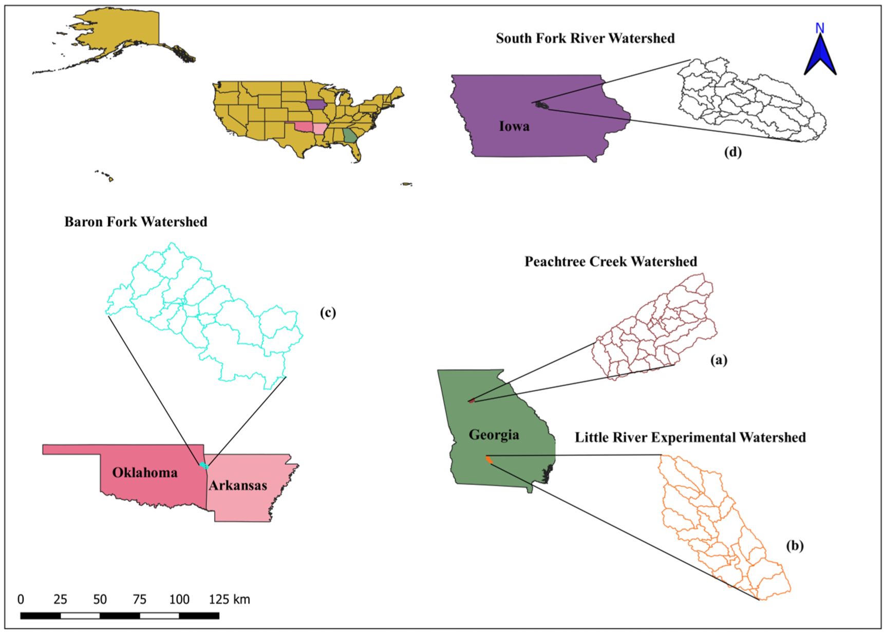
The four watersheds selected are (a) Peachtree Creek, (b) Little River, (c) Baron Fork, and (d) South Fork, based on different topographical/climate zones, as shown in Figure 2. The salient features of all four watersheds are presented in Table 1. For brevity, the analysis of the Peachtree Creek watershed is presented here. The Peachtree Creek watershed situated near Atlanta, Georgia, USA covers an area of 211.84 km2 with an average elevation of 299 m above mean sea level. According to the 2011 land-use dataset provided by the National Land Cover Database (NLCD), of 30 m resolution, the watershed is covered with an urban area of 86%. The primary soil of the watershed is red clayey soil. The climate is humid and subtropical in the watershed, with an average annual rainfall of 1200 mm and temperatures ranging from 44 °C to −15 °C. The monthly streamflow data were collected from the USGS monitoring station at the outlet point (USGS-02336300 Peachtree Creek at Atlanta, GA) for years 2000–2012. Precipitation data collected from TRMM and CFSR has spatial resolution of 0.25° and 30 km, respectively. The spatial resolution of DEM and LULC sources is 30 m. The details of the other three case studies are given in the Supplementary Material. The inputs are taken from three different sources, as shown in Table 2, and the total input model combinations developed from the sources are shown in Table 3.

Figure 2.
Location map of the four watersheds and their subbasins: (a) Peachtree Creek watershed, (b) Little River experimental watershed, (c) Baron Fork watershed, and (d) South Fork watershed.

Table 1.
Salient features of the four watersheds, including Climate, Slope, Area, and Mean Annual Precipitation (MAP).

Table 2.
List of input data collected for developing the SWAT model combinations.

Table 3.
List of input model combinations used in the study.
4. Results
This section discusses (i) Source uncertainty, (ii) Performance of the SWAT models, (iii) Parameter uncertainty, and (iv) Ranking of model combinations using MCDM in detail.
4.1. Source Uncertainty
4.1.1. DEM
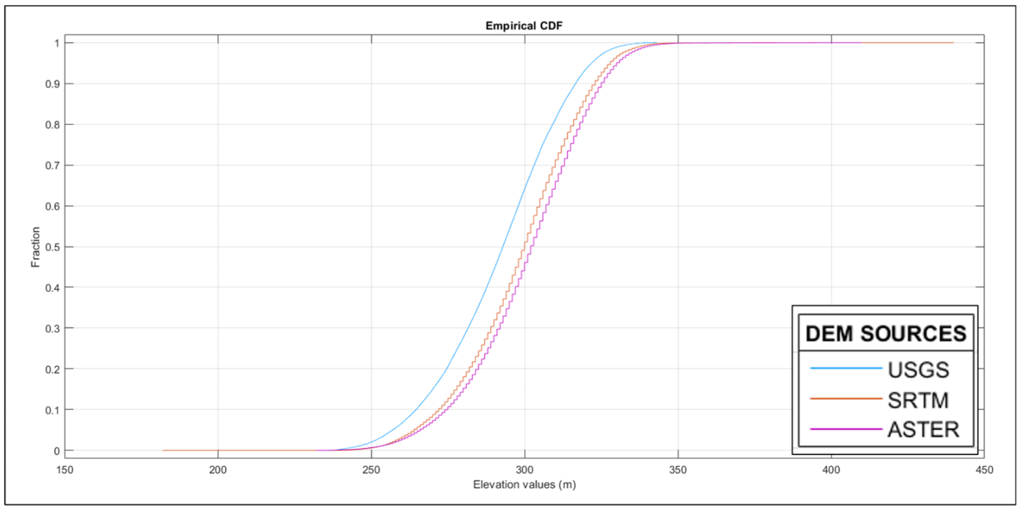
The input DEM sources show variation in elevation values for the watershed (Figure 3). SRTM provides the highest variation among all three, with USGS being the least variable. The variations are mainly due to the different vertical accuracy of the sources. Gesch et al. [40] compared the vertical accuracy of USGS (NED) DEM with the SRTM and ASTER DEM against the reference control points with the same vertical datum (North American Vertical Datum of 1988). The root mean square error (RMSE), a widely used error metric for documenting elevation data accuracy, expresses the overall absolute vertical accuracy [41]. The accuracy assessment results show SRTM and ASTER to be less accurate, with RMSE of 4.01 and 8.68 m, respectively, than the USGS (NED) DEM (RMSE: 1.84 m). Despite the lowest vertical accuracy, the ASTER DEM provides elevation values with a more refined range than SRTM. The results also support the significance of ASTER (Section 4). Furthermore, for steep slope, there is no significant variation in the elevation ranges among all three sources, and hence it can be concluded that there is no significant effect of DEM in the prediction of streamflows for steep slope (Section 4.4.3). The variation in DEM sources for other watersheds is provided in the Supplementary Material. The vertical accuracy of DEM varies according to the type of land cover [41]. As a result, different LULC sources are taken into account to study the combined effect, as these sources classify land use and land cover in different percentages.
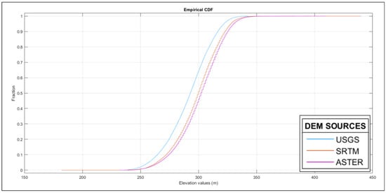
Figure 3.
Digital Elevation Model showing the minimum and maximum range for different sources.
4.1.2. LULC
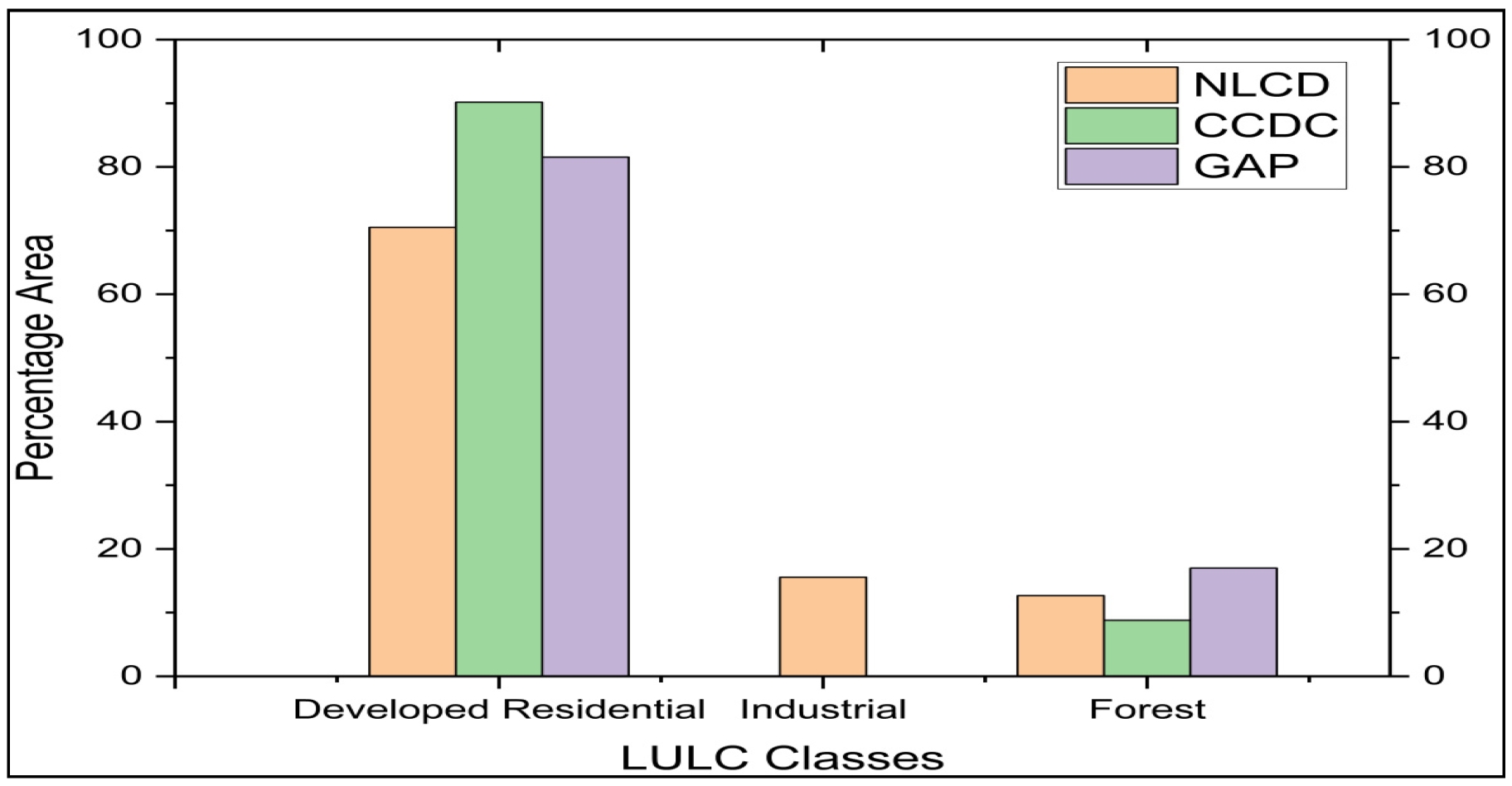
Among all three sources, NLCD land-use classification comprises of thirteen different classes, giving a more detailed and accurate classification followed by GAP and CCDC LULC (Figure 4). Hence, these variations in sources can also affect the accuracy of streamflow prediction and need to be quantified. From Figure 4, it is observed that according to the NLCD classification the area under industrial class is about 10% whereas the CCDC and GAP LULC sources is not depicting this land use classification for the Peachtree watershed. Similarly, the CCDC and GAP LULCs classify the area under residential class with approximately 30 and 15% higher than NLCD LULC classification, respectively. The variations in the different land classes is seen among the other three watersheds (Figure S3). Among all the watersheds the Little River (mild slope) watershed is showing higher variation in land-use classification for all the three LULCs and indicating the higher LULC source uncertainty as discussed in Section 4.4.2. For the study, an LULC of 2011 has been used due to negligible variations in the NLCD classes from 2001 to 2011 (Figure S1).
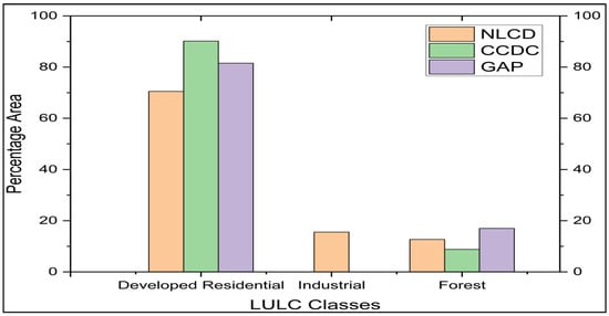
Figure 4.
Distribution of land use and land cover classes for the year 2011 as a percentage of total watershed area for three sources.
4.1.3. Precipitation
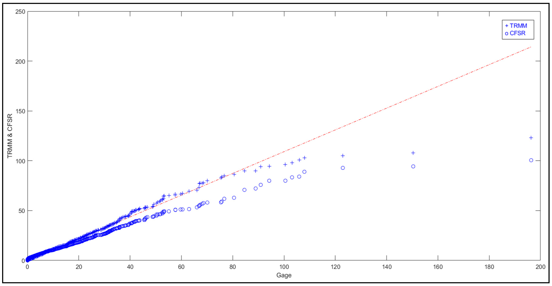
Another critical input for the SWAT model is the precipitation dataset. The CFSR data shows significant deviations from the Gage distribution and hence does not exhibit a linear distribution, while the TRMM dataset shows linearity to a more considerable extent and thus indicates a similar distribution as the Gage dataset (Figure 5). The precipitation collected from the CFSR data predicts higher values with low precipitation, and vice versa. The TRMM satellite data was able to follow the trend of gage data by capturing the precipitation to an appropriate level but is underpredicting at some periods, and hence is not able to capture the extremes as observed in the gage dataset, seen from Figure 5. Similarly, the CFSR dataset is also poor in replicating extremes, and thus both data sources are not satisfactory in capturing the extreme precipitation as per the Gage dataset. The variations in the precipitation sources for the other three watersheds are following a similar trend and can be seen in the Supplementary Material.
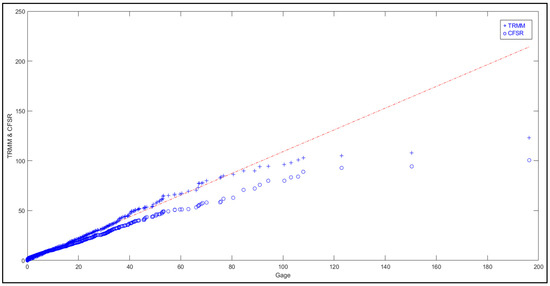
Figure 5.
TRMM and CFSR data are plotted against observed weather station (Gage) data to observe the trend on a daily time scale.
4.2. Performance of the SWAT Models
In the case of Peachtree, the analysis found that nine parameters were the most sensitive for streamflow prediction (Table 4).

Table 4.
Sensitive parameters obtained for the Peachtree region Creek Watershed from the global sensitivity analysis.
Impact of Uncertainties on Different Models
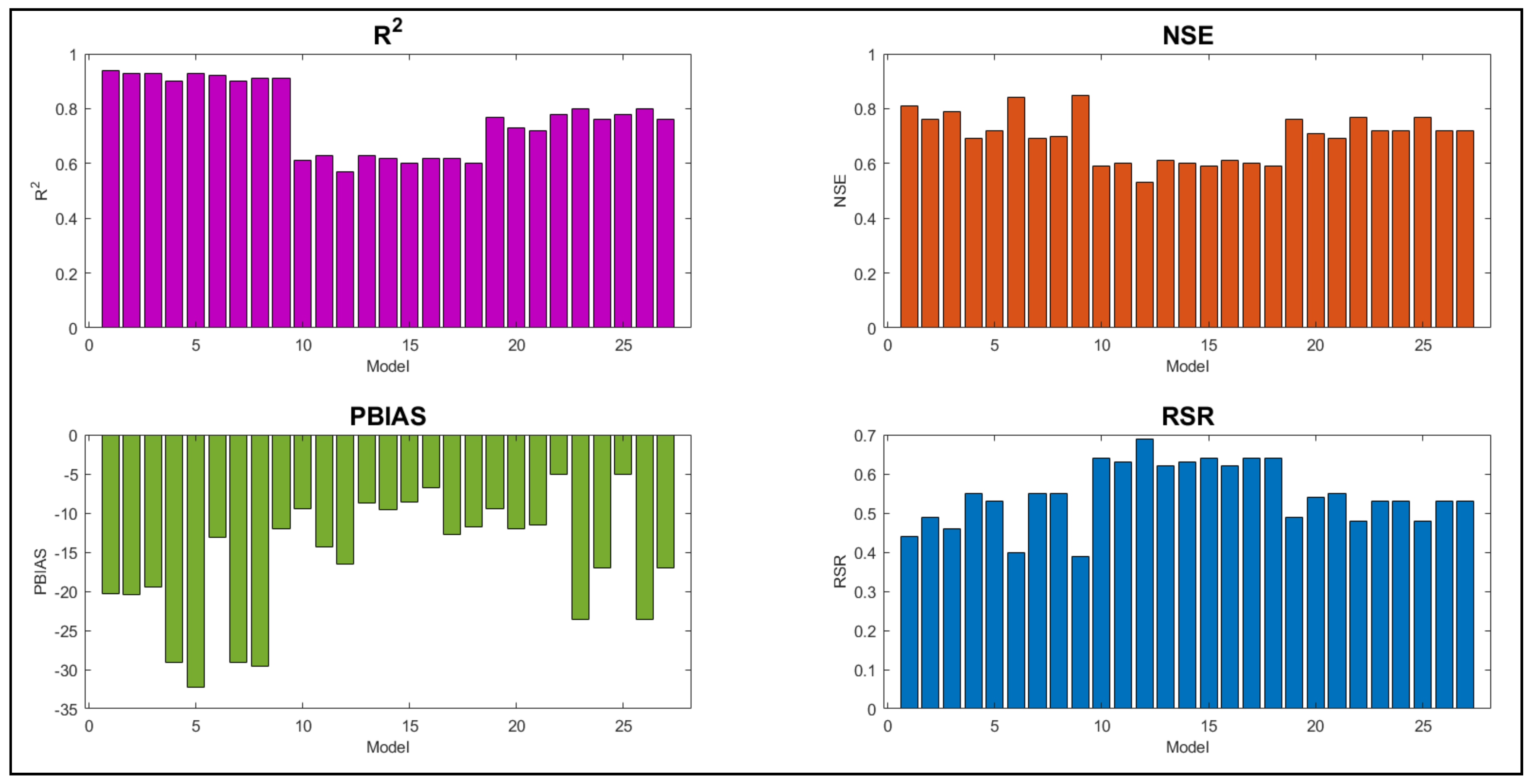
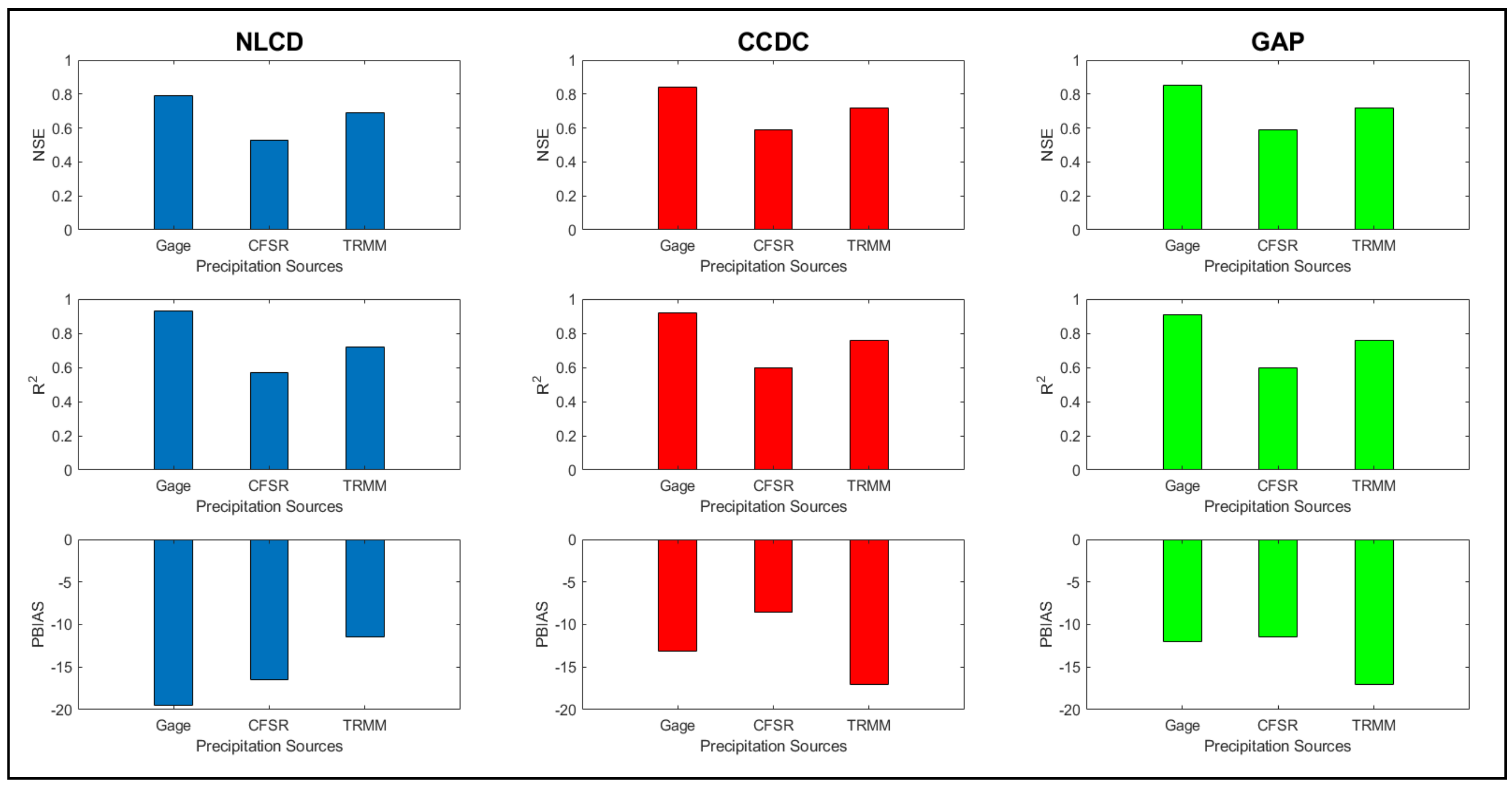
The NSE, R2, PBIAS, and RSR (Section 2.2) statistical indices quantify the source uncertainty associated with these inputs. From the analysis of 27 combinations (Figure 6), the Gage and TRMM precipitation combinations show good values for NSE, R2, and RSR statistical indices for the calibration and validation period compared to CFSR combinations. For the TRMM dataset, all statistical parameters give good results except PBIAS, which shows the highest overprediction followed by Gage but is less than the defined limit of 25%. However, CFSR combinations give better PBIAS values for the calibration and validation period (Figure 7), but do not correlate well with the observed flows. Overall, the ASTER DEM with NLCD LULC for the TRMM dataset gives the best result, while for the validation period, ASTER DEM, in combination with the Gage dataset, gives the best results for CCDC and GAP LULC (Figure 7-Combination: 6 & 9). The combinations gave good NSE (0.85 & 0.84), R2 (0.92 & 0.91) and PBIAS (−12 & −13%) values for validation followed by USGS DEM with NLCD LULC and Gage precipitation combination (Figure 7-Combination: 1) with NSE as 0.81 and PBIAS as −20%. Among the CFSR dataset, the USGS DEM gives better results for all the objective functions relatively with maximum NSE and R2 and minimum PBIAS and RSR. The CFSR dataset yielded poor performance with any combination and hence can be given the least priority when considering the precipitation datasets.
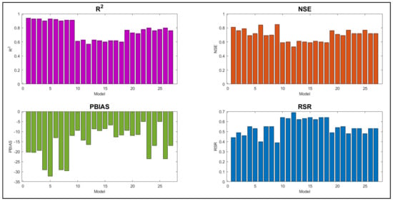
Figure 6.
SWAT model performance for the 27 combinations with the four performance criteria (R2, NSE, PBIAS, and RSR) for the calibration period.
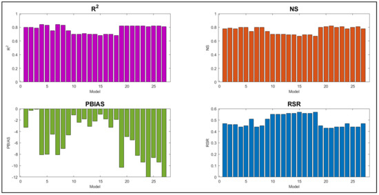
Figure 7.
SWAT model performance for the 27 combinations shown with the four performance criteria (R2, NSE, PBIAS, and RSR) for the validation period.
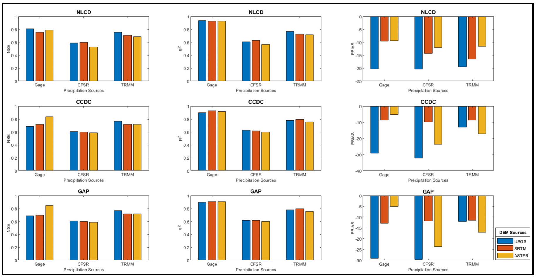
When considering the NSE value, all the DEMs for NLCD LULC provide the best result for the Gage combination followed by TRMM, while the least results were obtained from the CFSR datasets (Figure 8). For CCDC LULC, ASTER gives the best results with Gage datasets and the least with the CFSR one. The same trend is observed from the results obtained for the GAP LULC. The satellite data is giving satisfactory results with all the DEMs and LULCs. There is a good correlation between USGS DEM and TRMM data, as the DEM is performing well irrespective of LULC. For more detailed and accurate quantification of the source uncertainty, the LULC and precipitation sources are compared, keeping the DEM source constant. The detailed analysis for each DEM source is presented below.
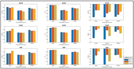
Figure 8.
DEM and precipitation dataset comparison based on NSE, R2, and PBIAS values for NLCD; CCDC; and GAP LULC.
USGS DEM
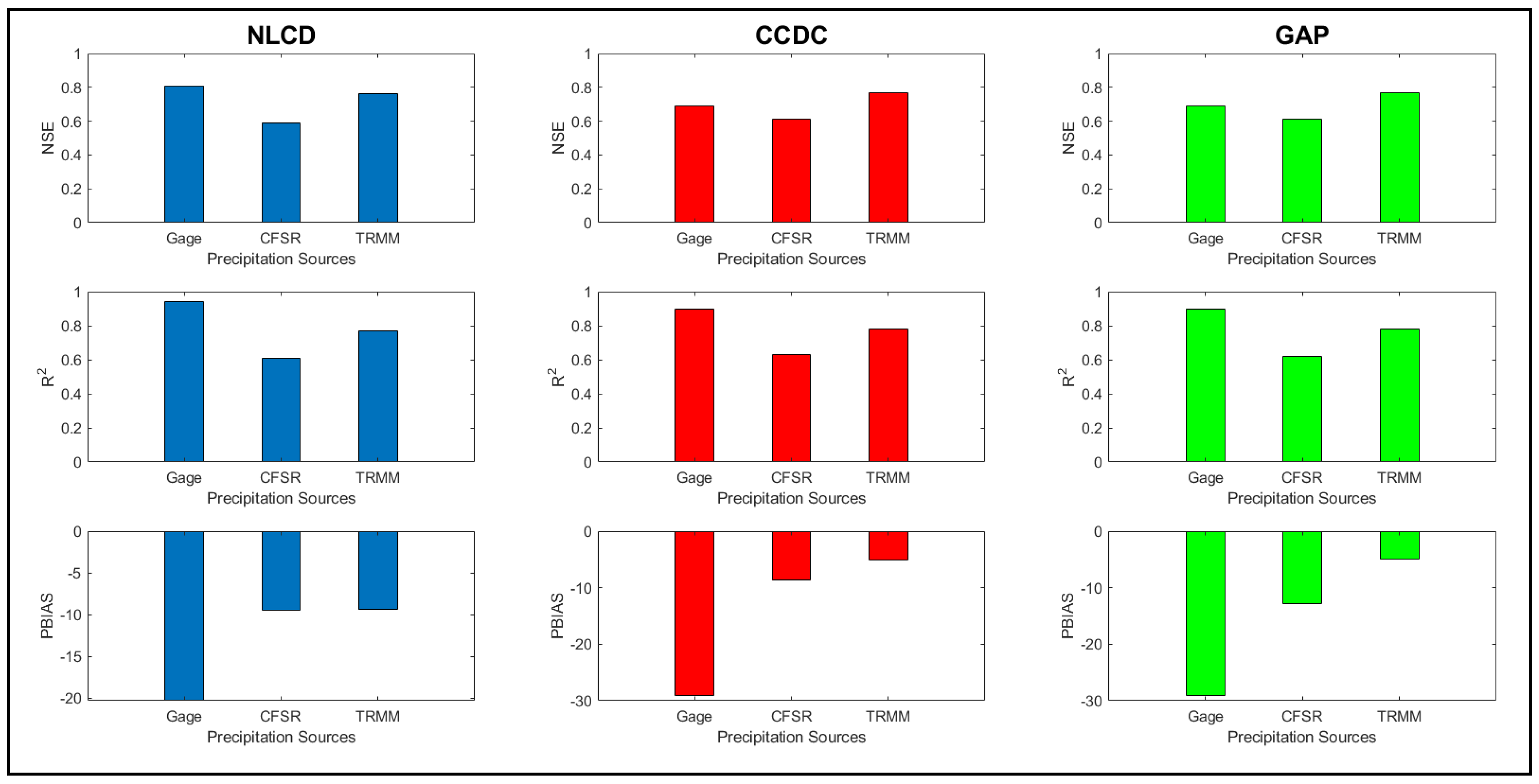
The NLCD LULC performs better with the USGS DEM for the Gage dataset (Figure 9). The NSE value of 0.81 for the respective LULC is relatively higher (15%) than the other two (0.69 for CCDC and GAP). Moreover, the CCDC and GAP LULC produce the same results with the respective gage dataset. For the CFSR dataset, there is a slight difference between the NLCD and the other two LULCs, giving 3% higher NSE and R2 than NLCD.
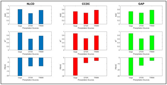
Figure 9.
Model performance with various LULC and precipitation dataset combinations for the USGS DEM based on NSE, R2, and PBIAS criteria.
When considering the PBIAS value, the CCDC shows the least value (−8.7%) followed by NLCD (−9.5%), and GAP being the highest with (−12.8%). Overall, the CCDC LULC produces the best results for the precipitation dataset and DEM. For the satellite TRMM dataset, when considering NSE, RSR, and R2, all LULCs are performing well, but when considering PBIAS value, GAP and CCDC LULCs provide entirely satisfactory results (5%).
SRTM DEM
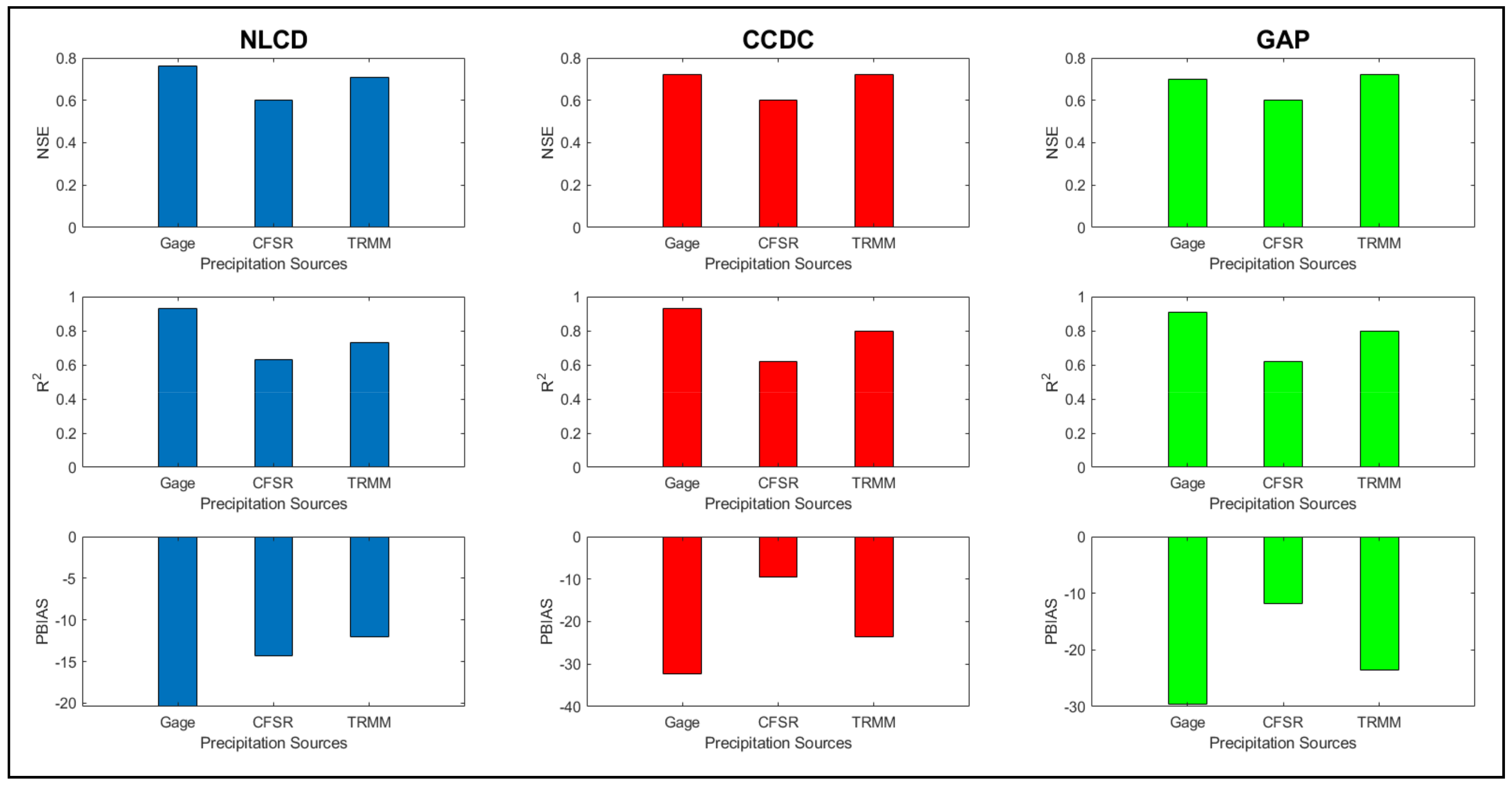
The NLCD LULC gives the best NSE values (0.76) for the Gage dataset (Figure 10). Other than NSE, R2, PBIAS, and RSR values also show promising results for the respective LULC with 0.93, −20.4%, and 0.49, respectively, followed by CCDC LULC with 0.76 as NSE and 0.93 as R2. The GAP LULC produces poor results with the respective gage dataset among all the LULCs. For the CFSR dataset, there is no change in NSE (0.6), R2 (0.63), and RSR (0.63) values for all LULCs, which shows that the SRTM DEM can be used with any of the LULC for the reanalysis dataset. When considering the PBIAS value, the CCDC gives the least overprediction value (−9.6%), followed by GAP (−11.8%), and NLCD being the highest (−14.3%). Overall, the CCDC LULC produces the best results for the precipitation dataset and DEM. For the satellite dataset, when considering the NSE, RSR, and R2, all LULCs are performing well, but when considering the PBIAS value, the NLCD LULC is performed much better (12%) at giving the least overprediction. than the CCDC and GAP LULCs (−24%).
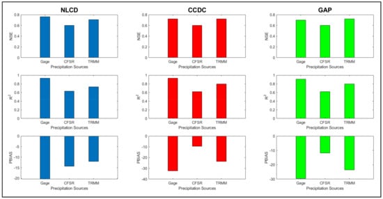
Figure 10.
Model performance with various LULC and precipitation dataset combinations for the SRTM DEM based on NSE, R2, and PBIAS criteria.
ASTER DEM
The ASTER DEM performs well with the CCDC and GAP LULC for all the precipitation combinations. For Gage data, the CCDC and GAP LULC provide better results for the three indices (Figure 11). The DEM with NLCD LULC gives the least overprediction (PBIAS: −11.5%) in culmination with the TRMM dataset, which is way better than the other LULCs (PBIAS: −17%). Overall, the ASTER DEM should be used with the CCDC and GAP LULC for the Gage and NLCD for TRMM and CFSR.
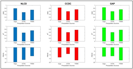
Figure 11.
Model performance with various LULC and precipitation dataset combinations for the ASTER DEM based on NSE, R2, and PBIAS criteria.
The calibrated model fits the influential parameters with a varying range for the same region as per the input combination and is quantified as the parameter uncertainty in the study (Section 4.3).
4.3. Parameter Uncertainty
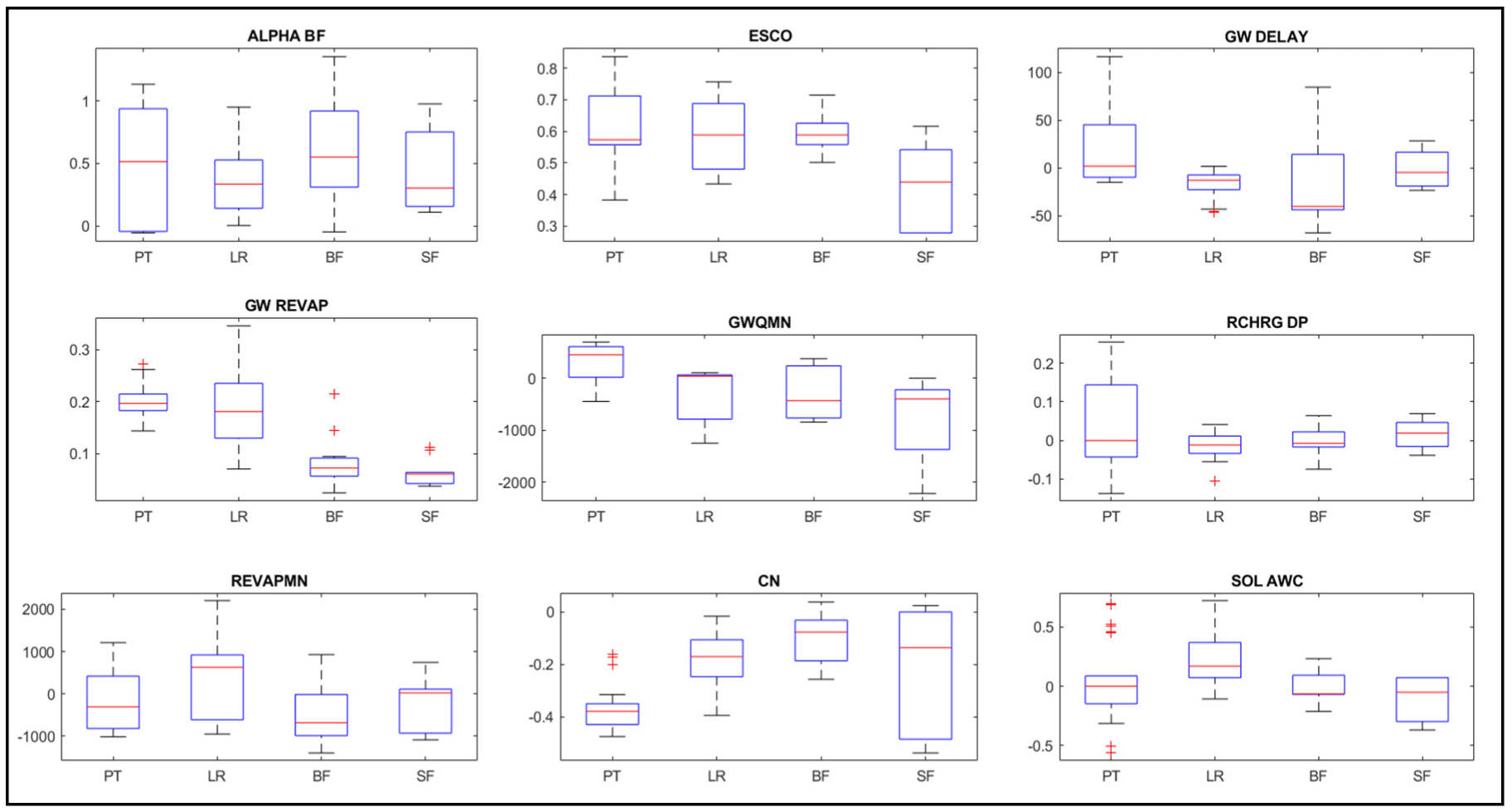
Figure 12 shows the box plot of the selected nine sensitive parameters for all of the watersheds (Figure 12). It is evident that the different models’ combinations choose the different fit values of the parameters for the same region. The variation in the input sources can be seen from the parameters used to calibrate the streamflows, as all other processes are kept constant while building the model. The range for ALPHA_BF, GWQMN, and REVAPMN vary for different models and hence shows more uncertainty than other parameters for all four case studies used in the paper. The more the range variation, the more the uncertainty in the models can be expected. The curve number (CN) is not varying significantly for all watersheds except the South Fork watershed, where the interquartile ranges are relatively large, which shows higher uncertainty. Also, the available water capacity in the soil layer varies for the region, and hence both groundwater parameters and CN shows significant variations. This indicates that LULC sources have more effect in the region. For the Peachtree watershed, the outliers for the CN show that some combination models, especially SRTM DEM with NLCD LULC with CFSR and TRMM datasets provide the least CN value for the region, while the ASTER DEM with CCDC and GAP LULCs plus the TRMM dataset provides the highest CN value. The region has more variation in the groundwater parameters and the CN parameter, and it can be stated that the choice of DEM source in culmination to LULC affects the streamflow prediction ability. For Baron Fork, as the slope is steep, significant variation is seen in the parameters depicting topography. Hence, the higher uncertainty induced in the flow simulation is due to different DEM sources. The mild slope (Little River watershed) is affected by both the DEM and LULC sources. Furthermore, the region’s tropical climate emphasizes the importance of snow parameters (Figure S26).
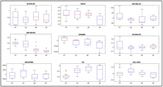
Figure 12.
Variation of nine selected influential parameters for the model combinations used in the four watersheds: Peachtree (PT), Little River (LR), Baron Fork (BF), South Fork (SF).
4.4. Quantification of Simulated Flows
4.4.1. Peachtree Creek Watershed
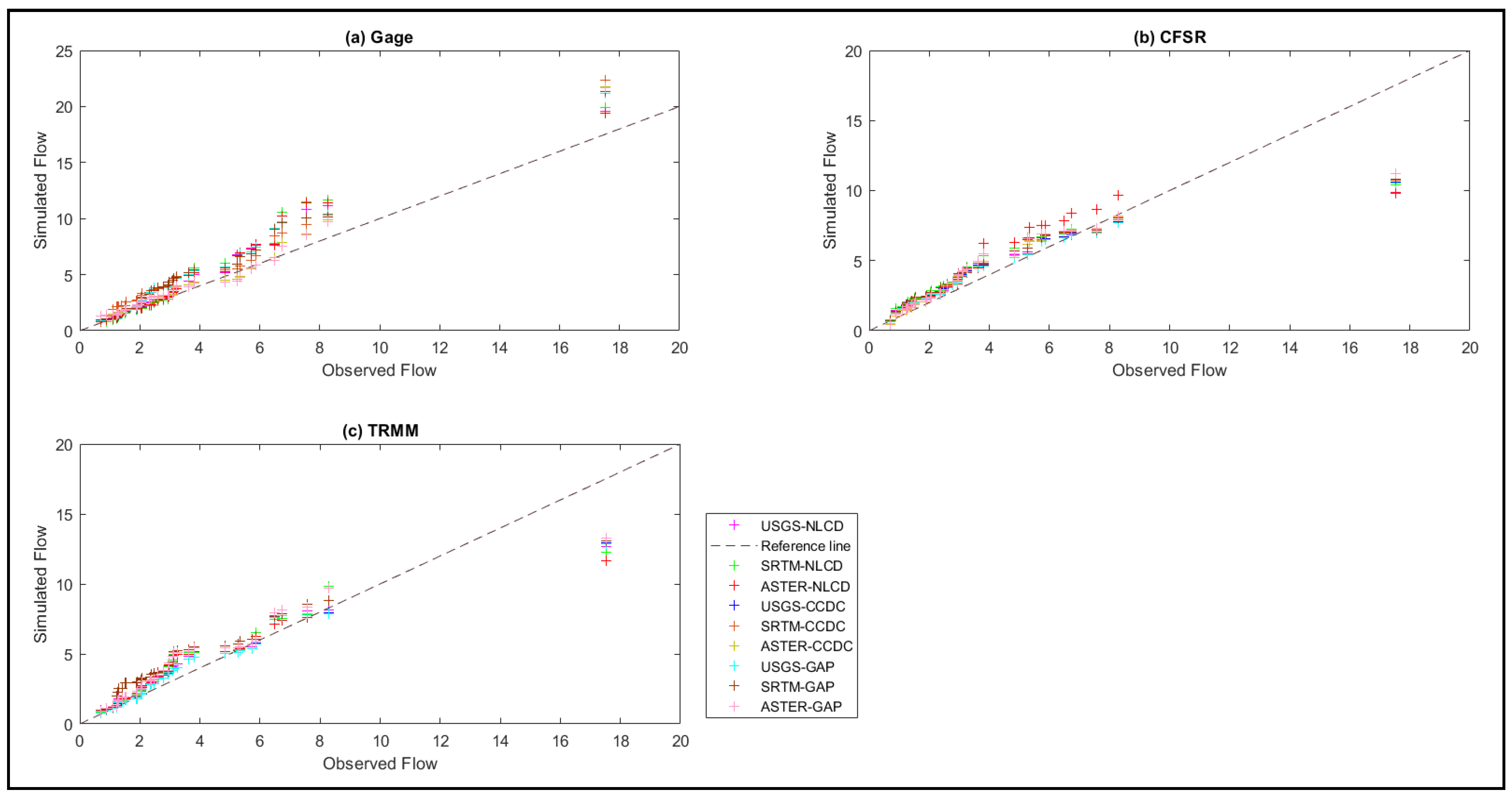
From Figure 13a–c, it is seen that all combinations of gage datasets simulate the highest flow in the range of 19 to 22 cumecs for the validation period, while the highest flow observed from the stream gage station is around 17.5 cumecs. Hence, the dataset overpredicts the higher flows while the TRMM dataset simulates 12 to 13 cumecs. The CFSR dataset cannot simulate the high flows, and combinations give high flows in the range of 9 to 11 cumecs only, and hence it may not be suitable for the prediction of stream flows. All datasets can capture the low discharge values well. Based on LULCs, the plot shows that all combinations of NLCD LULC are simulating higher flows less than the other two LULCs for any precipitation dataset. The reason for the lower discharge values obtained from NLCD LULC is due to the refined classification compared to other LULCs. The USGS DEM also simulates less for every precipitation dataset and LULC, while ASTER DEM predicts more high flows other than the gage dataset with NLCD LULC. The major reason for the variation in DEMs is due to the vertical accuracy of the DEM. The ASTER DEM is giving good results with NLCD LULC and the gage dataset due to the least error in the other two datasets, which in combination predicts the flows with lower uncertainty when compared with other ASTER DEM combinations. Overall, the USGS DEM with NLCD LULC predicts high flows closer to observed ones.

Figure 13.
Variation of simulated flows with observed flows was obtained for the three precipitation datasets as (a) Gage, (b) CFSR, and (c) TRMM with nine different combinations for the Peachtree watershed.
4.4.2. Little River Experimental Watershed
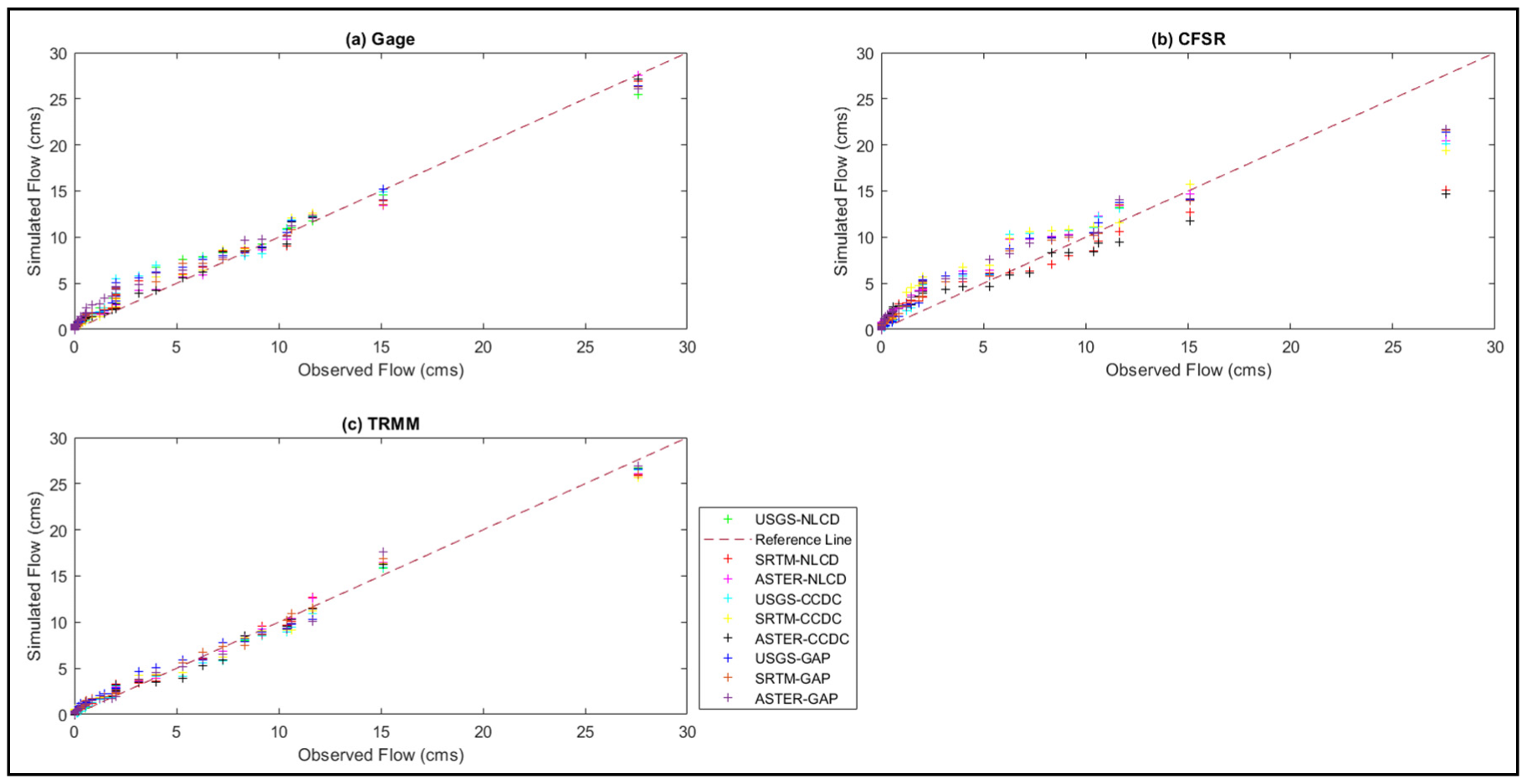
The gage and TRMM datasets simulate high flows from 25 to 28 cumecs, while the observed highest flow from the stream gage station is around 27.59 cumecs (Figure 14). Combination 3 (ASTER DEM with NLCD LULC and Gage precipitation) can simulate the highest streamflow perfectly with the observed one. The combinations with the CFSR dataset are giving high flows in the range of 15 to 22 cumecs, and hence do not simulate the high flows satisfactorily. All datasets can capture the low flows well. The plots (Figure S11) indicates that for any precipitation dataset all combinations of NLCD LULC are simulating higher flows more diminutive than the other two LULC sources.
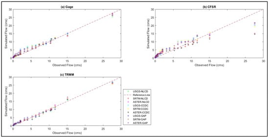
Figure 14.
Variation of simulated flows with observed flows was obtained for the three precipitation datasets as (a) Gage, (b) CFSR, and (c) TRMM with nine different combinations for the Little River watershed.
4.4.3. Baron Fork Watershed
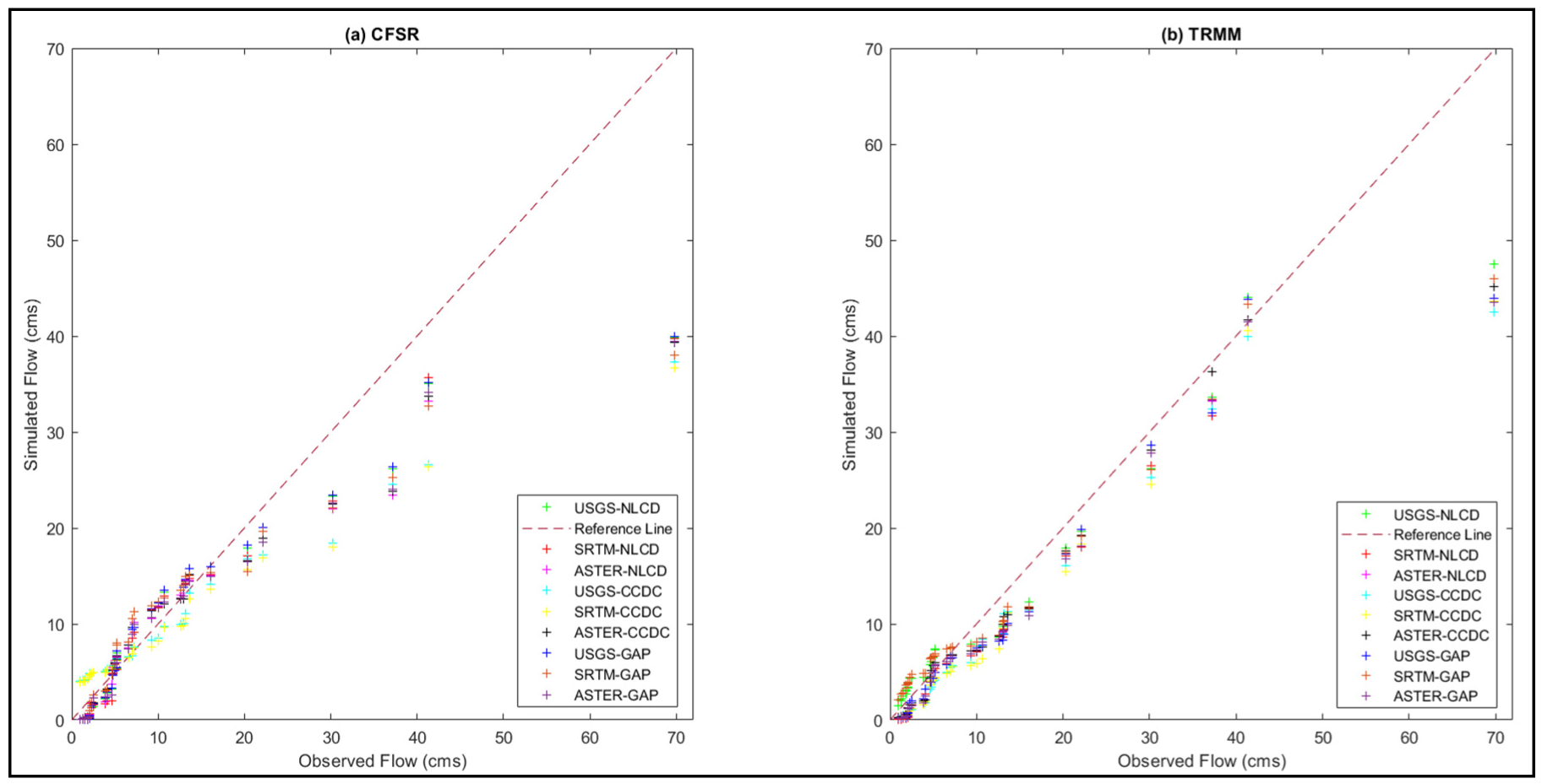
The combinations of TRMM datasets provide better streamflow simulations than CFSR ones (Figure 15a,b). It can clearly be stated that both the datasets cannot capture the high flows, while TRMM combinations are simulating high flows better than the CFSR combinations. The USGS DEM shows good predictions with all the LULCs for both precipitation datasets. When considering LULCs, the CFSR data is behaving well with CCDC and GAP LULC, similar to the Peachtree watershed.
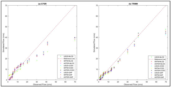
Figure 15.
Variation of simulated flows with observed flows was obtained for the two precipitation datasets: (a) CFSR and (b) TRMM, with nine different combinations for the Baron Fork watershed.
4.4.4. South Fork Watershed
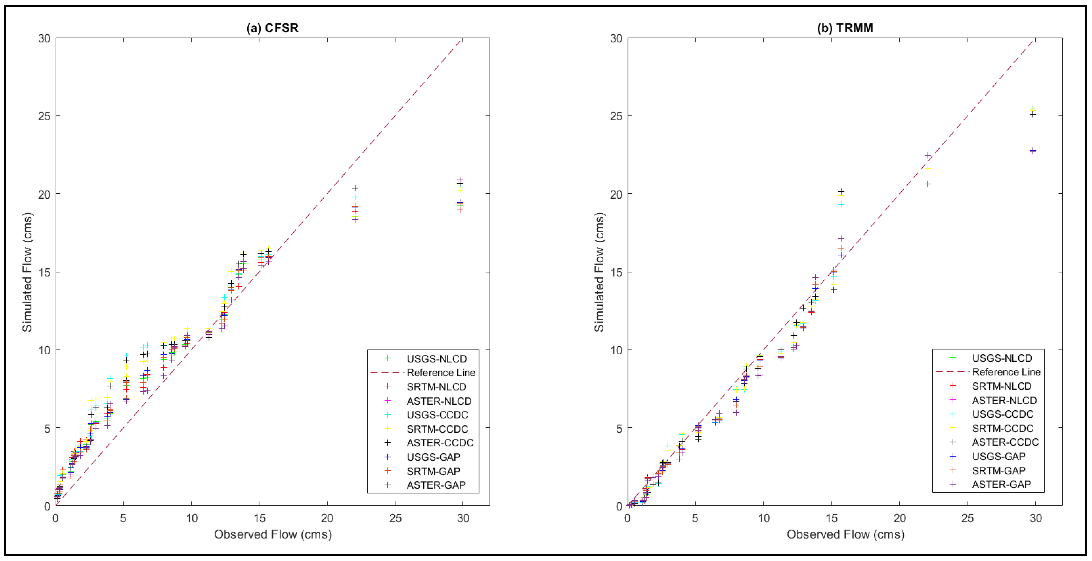
Both precipitation combinations provide satisfactory results for the region, but the TRMM combinations capture the flows better. The ASTER DEM with GAP LULC simulates high flows closer to actual stream gage data, followed by USGS and SRTM with NLCD and CCDC LULC, respectively, for the satellite dataset. Some combinations are overpredicting for TRMM, while all CFSR combinations overpredict the low flows. When considering the performance of all statistical indices, it can be concluded that the TRMM datasets can be used to predict streamflow behavior (Figure 16).
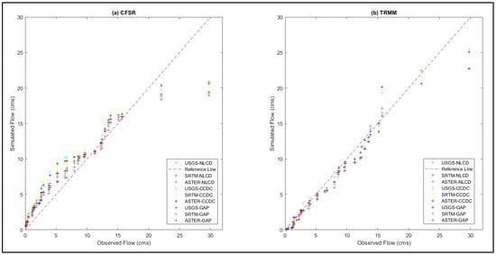
Figure 16.
Variation of simulated flows with observed flows was obtained for the two precipitation datasets: (a) CFSR and (b) TRMM, with nine different combinations for the South Fork watershed.
The efficiency of different model combinations having NSE values greater than 0.75 is shown in Figure 17. The USGS DEM combinations are seen in greater numbers than other combinations when considering NSE values greater than 0.75 for all four watersheds. USGS DEM performs best with TRMM data irrespective of LULC. Similarly, ASTER behaves best with the Gage data. SRTM and USGS give good results with NLCD LULC for the Gage dataset. Among all the four watersheds it can be seen that the TRMM data is providing satisfactory results and can be used for the prediction of streamflows. The combinations of the CFSR dataset are not able to provide the efficiency of 0.75 and hence are the least preferred among all combinations.
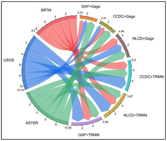
Figure 17.
Plot showing the efficiency of combinations irrespective of climatic and topographical regions for NSE > 0.75.
The simulation results for the other three case studies (Little River, Baron Fork, and South Fork) are provided in the Supplementary Material. It is arduous and complex to determine the best combination for the case studies taking into account all statistical indices. As a result, the MCDM approach ranks the best combinations, as shown in the following subsection.
4.5. Multi-Criteria Decision Making (MCDM) Analysis
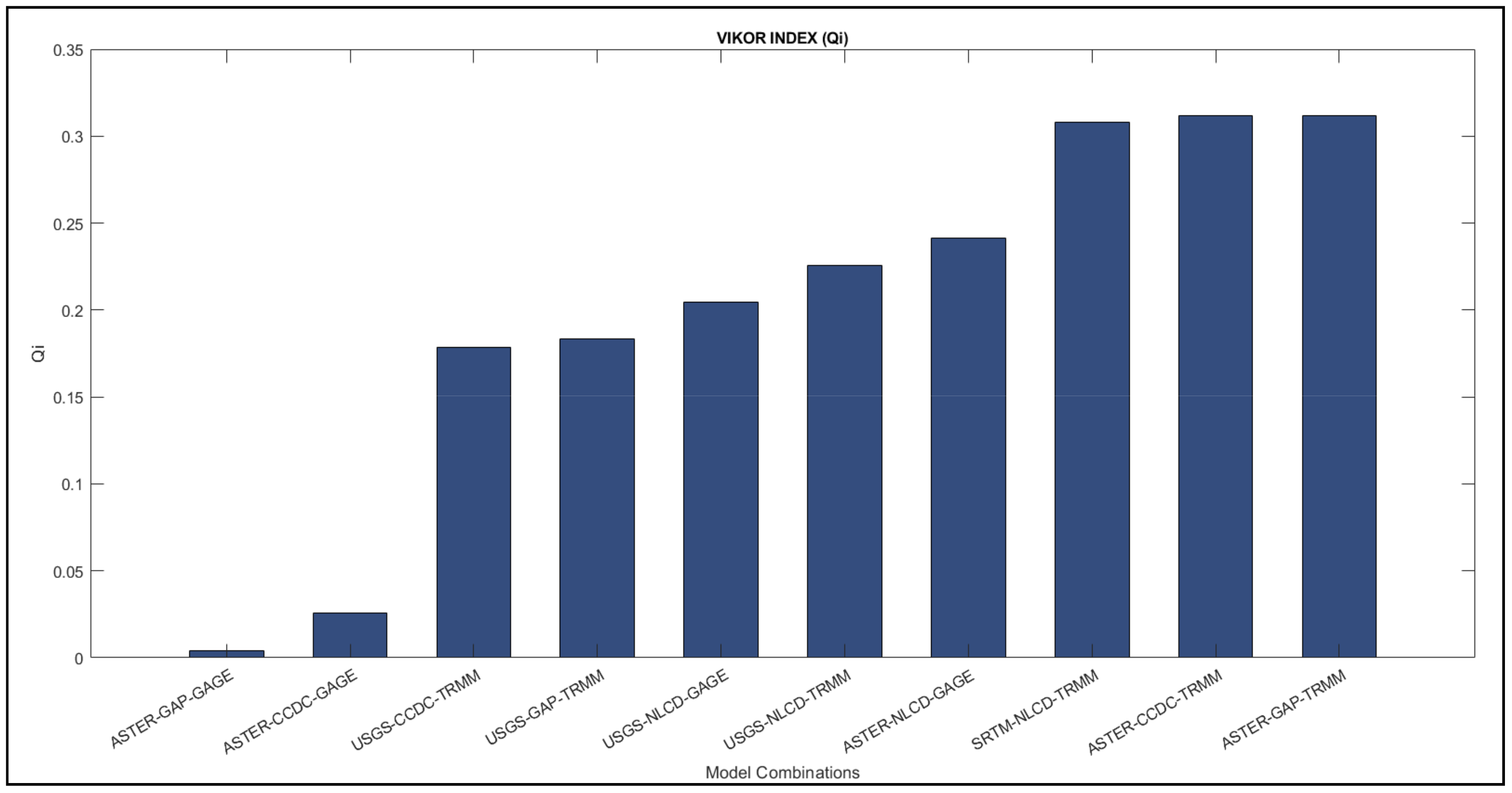
The nine statistical indices are used as criteria and are weighted by the equal weight method. The 27 model combinations are then ranked by the VIKOR MCDM method concerning statistical indices. The alternatives with the lowest VIKOR index give the best option (Figure 18).

Figure 18.
VIKOR index (Qi) values were obtained for different model combinations. The model with minimum value is considered as close to the optimal alternative.
Each statistical indicator reflects the model’s fitness with the observed data. For example, based on various studies [42,43], the model performance is considered satisfactory if threshold values for PBIAS , . The SSQR value closer to 0 indicates that the model is more fit for prediction. Hence, it is necessary to combine the information contained in all the indices for evaluating the model performance. Therefore, equal weight is assigned to all nine criteria.
The ranking by the MCDM method shows that the best input combination suitable for the Peachtree watershed is ASTER DEM with the GAP LULC and Gage dataset, followed by the same DEM with the CCDC LULC and the Gage dataset only (Figure 18). The combination of USGS DEM with CCDC and TRMM data shows a good performance for the watershed (Table S1). Both the and NSE values of these model combinations are more than 0.8. The SSQR values are 0.076 and 0.081, respectively, for these models. These rankings show an agreement between the VIKOR and validation analysis presented in the previous subsections, proving the VIKOR’s efficacy. The precipitation datasets such as Gage and TRMM claim higher priority compared to CFSR. For other watersheds (Little River, Baron Fork, and South Fork), USGS DEM with the TRMM dataset attained the highest ranking from the method. The ranking tables (Tables S1–S4) for the combinations of all the watersheds are provided in the Supplementary Material.
5. Conclusions
The accurate simulation of streamflow is paramount for relevant decision-making in water resources management. This paper presents the uncertainty analysis associated with the input sources for different topographical and climatic regions in streamflow prediction using the SWAT model. Different model combinations were studied to quantify the integrated impact of DEM, LULC and precipitation datasets in the prediction of streamflows. The studied input combinations were prioritized based on VIKOR MCDM to find the alternatives with least uncertainty. The study also showed the model’s robustness and applicability in different regions. The SWAT model provided excellent and satisfactory results for all combinations used in the case studies taking into account all statistical indices.
Highlights of the SWAT-MCDM Analysis
(1) Overall, USGS DEM simulates streamflow best with the NLCD LULC for TRMM and CFSR precipitation. ASTER DEM performs well with CCDC and GAP LULC for any precipitation dataset, while SRTM performs well with NLCD LULC.
(2) The Gage dataset gives the best performance for the case studies, followed by TRMM, with CFSR giving the poorest. The CFSR dataset over-predicts the low precipitation values, while TRMM captures precipitation as observed in the gauge dataset to an appropriate degree.
(3) The LULC does not significantly affect the discharge for the moderately sloped watersheds like Peachtree and South Fork but contributes more uncertainty for the mild slope (Little River).
(4) Although the DEM sources significantly affect the streamflow for all topographic regions except the steep slope, where the impact of DEM and LULC sources is minimal, the steep slope region is more sensitive to the precipitation sources followed by DEM.
(5) Higher uncertainty is observed in the simulation of high flows compared to low flows. Hence, extremes are not captured well by the input data sources.
(6) The TRMM data became a more reliable dataset without an observed station dataset to predict streamflow. TRMM data provides a good correlation of predicted flows with the observed flow. All combinations of this dataset provide lower uncertainty in streamflow simulation than others.
(7) The parameters used for streamflow prediction also show uncertainties that directly describe the variation in sources. The parameters influencing sub-surface flows such as ALPHA_BF, GWQMN, and REVAPMN show higher uncertainty compared to others. These groundwater parameters are highly sensitive to variations in topography (slope), land-use/land-cover and precipitation. This emphasizes the need to quantify uncertainty associated with all three input sources (DEM, LULC and precipitation datasets) for accurate prediction of streamflows.
(8) USGS DEM with NLCD and CCDC LULC ranked at the top among all model combinations in the MCDM analysis.
Although the uncertainty caused by the DEM is smaller than the uncertainty caused by precipitation, it can be concluded that the DEM and precipitation datasets are significant sources contributing to overall input uncertainty. The combinations are considered based on different sources of DEM, LULC, and precipitation in the study. Different resolutions of the inputs can be added to quantify the overall input uncertainty as an extension to the study. As the most common sources of DEM and LULC are incorporated into the study, more combinations can be created by combining them with other additional sources. In addition, the soil and temperature sources are left unexplored in the research and can be studied further. The uncertainty in different climatic models can be quantified in addition to existing precipitation sources. The study can also be conducted in the mountainous region (average slope > 605 m), which is currently unexplored in the present work.
Supplementary Materials
The following supporting information can be downloaded at: https://www.mdpi.com/article/10.3390/rs14215385/s1. References [44,45,46] are cited in the supplementary materials.
Author Contributions
Conceptualization, R.S.; methodology, J.C., U.R.P. and R.S.; software, J.C. and U.R.P.; validation, J.C., U.R.P. and R.S.; formal analysis, J.C., U.R.P. and R.S.; investigation, J.C. and R.S.; resources, R.S.; data curation, J.C., R.U.S. and U.R.P.; writing—original draft preparation, U.R.P. and J.C.; writing—review and editing, R.U.S. and R.S.; visualization, R.U.S. and R.S.; supervision, R.S.; project administration, U.R.P., R.U.S. and R.S.; funding acquisition, R.U.S. and R.S. All authors have read and agreed to the published version of the manuscript.
Funding
This research received no external funding.
Data Availability Statement
Not applicable.
Acknowledgments
The authors would like to express their gratitude to the anonymous reviewers for constructive feedback and comments. The first two authors would like to thank Debayan Mandal, Texas A&M University for his initial support in the discussions of SWAT model and also HydroSystems Research group, IIT Tirupati for their support.
Conflicts of Interest
The authors declare that they have no conflict of interest.
References
- Arnold, J.; Srinivasan, R.; Muttiah, R.; Williams, J. Large area hydrologic modeling and assessment part i: Model development. J. Am. Water Resour. Assoc. 1998, 34, 73–89. [Google Scholar] [CrossRef]
- Gassman, P.; Reyes, M.; Green, C.; Arnold, J. The soil and water assessment tool: Historical development, applications, and future research directions. Trans. ASABE 2007, 50, 1211–1250. [Google Scholar] [CrossRef]
- Knisel, W. Creams: A Field-Scale Model for Chemicals, Runoff, and Erosion from Agricultural Management Systems; Conservation Research Report. 26; USDA: Washington, DC, USA, 1980. [Google Scholar]
- Leonard, R.; Knisel, W.; Smith, D. Gleams: Groundwater loading effects of agricultural management systems. Trans. ASAE 1987, 30, 1402–1418. [Google Scholar] [CrossRef]
- Arnold, J.; Williams, J.; Nicks, A.; Sammons, N. Swrrb: A Basin-Scale Simulation Model for Soil and Water Resources Management; Texas AM University Press: College Station, TX, USA, 1990. [Google Scholar]
- Zuoda, Q.; Kang, G.; Chu, C.; Qiu, Y. Comparison of swat and gwlf model simulation performance in humid south and semi-arid north of china. Water 2017, 9, 567. [Google Scholar]
- Jaiswal, R.; Ali, S.; Bharti, B. Comparative evaluation of conceptual and physical rainfall-runoff models. J. Appl. Water Sci. 2020, 10, 48. [Google Scholar] [CrossRef]
- Nasiri, S.; Ansari, H.; Ziaei, A. Simulation of water balance equation components using swat model in samalqan watershed (Iran). Arab. J. Geosci. 2020, 13, 421. [Google Scholar] [CrossRef]
- Cotter, A.; Chaubey, I.; Costello, T.; Soerens, T.; Nelson, M. Water quality model output uncertainty as affected by spatial resolution of input data. J. Am. Water Resour. Assoc. 2003, 39, 977–986. [Google Scholar] [CrossRef]
- Yin, Z.; Xiao, H.; Zou, S.; Zhu, R.; Lu, Z.; Lan, Y.; Shen, Y. Simulation of hydrological processes of mountainous watersheds in inland river basins: Taking the Heihe mainstream river as an example. J. Arid. Land 2013, 6, 16–24. [Google Scholar] [CrossRef]
- Kumar, B.; Lakshmi, V.; Patra, K.C. Evaluating the Uncertainties in the SWAT Model Outputs due to DEM Grid Size and Resampling Techniques in a Large Himalayan River Basin. J. Hydrol. Eng. 2017. [Google Scholar] [CrossRef]
- Fan, J.; Galoie, M.; Motamedi, A.; Huang, J. Assessment of land cover resolution impact on flood modeling uncertainty. Water Policy 2021, 52, 78–90. [Google Scholar] [CrossRef]
- Gautam, S.; Dahal, V.; Bhattarai, R. Impacts of Dem Source, Resolution and Area Threshold Values on SWAT Generated Stream Network and Streamflow in Two Distinct Nepalese Catchments. Environ. Process 2019, 6, 597–617. [Google Scholar] [CrossRef]
- Munoth, P.; Goyal, R. Effects of DEM Source, Spatial Resolution and Drainage Area Threshold Values on Hydrological Modeling. Water Resour. Manag. 2019, 33, 3303–3319. [Google Scholar] [CrossRef]
- Sukumaran, H.; Sahoo, S.N. A Methodological Framework for Identification of Baseline Scenario and Assessing the Impact of DEM Scenarios on SWAT Model Outputs. Water Resour. Manag. 2020, 34, 4795–4814. [Google Scholar] [CrossRef]
- Kamali, B.; Abbaspour, K.; Lehmann, A.; Wehrli, B.; Yang, H. Assessing the uncertainty of multiple input datasets in the prediction of water resource components. Water 2017, 9, 709. [Google Scholar] [CrossRef]
- Cüceloğlu, G.; Seker, D.Z.; Tanik, A.; Öztürk, I. Analyzing Effects of Two Different Land Use Datasets on Hydrological Simulations by Using SWAT Model. Int. J. Environ. Geoinform. 2021, 8, 172–185. [Google Scholar] [CrossRef]
- Alnahit, A.O.; Mishra, A.K.; Khan, A.A. Evaluation of high-resolution satellite products for streamflow and water quality assessment in a Southeastern US watershed. J. Hydrol. Reg. Stud. 2020, 27, 100660. [Google Scholar] [CrossRef]
- Le, M.; Lakshmi, V.; Bolten, J.; Bui, D.D. Adequacy of Satellite-derived Precipitation Estimate for Hydrological Modeling in Vietnam Basins. J. Hydrol. 2020, 586, 124820. [Google Scholar] [CrossRef]
- Dinh, K.D.; Anh, T.N.; Nguyen, N.Y.; Bui, D.D.; Srinivasan, R. Evaluation of Grid-Based Rainfall Products and Water Balances over the Mekong River Basin. Remote Sens. 2020, 12, 1858. [Google Scholar] [CrossRef]
- Zhang, L.; Xin, Z.; Zhou, H. Assessment of TMPA 3B42V7 and PERSIANN-CDR in Driving Hydrological Modeling in a Semi-Humid Watershed in Northeastern China. Remote Sens. 2020, 12, 3133. [Google Scholar] [CrossRef]
- Setti, S.; Maheswaran, R.; Sridhar, V.; Barik, K.; Merz, B.; Agarwal, A. Inter-Comparison of Gauge-Based Gridded Data, Reanalysis and Satellite Precipitation Product with an Emphasis on Hydrological Modeling. Atmosphere 2020, 11, 1252. [Google Scholar] [CrossRef]
- Dutta, P.; Sarma, A.K. Hydrological modeling as a tool for water resources management of the data-scarce Brahmaputra basin. J. Water Clim. Chang. 2020, 12, 152–165. [Google Scholar] [CrossRef]
- Beven, K.; Binley, A. The future of distributed models: Model calibration and uncertainty prediction. Hydrol. Process. 1992, 6, 279–298. [Google Scholar] [CrossRef]
- Van Griensven, A.; Meixner, T. Methods to quantify and identify the sources of uncertainty for river basin water quality models. Water Sci. Technol. 2006, 53, 51–59. [Google Scholar] [CrossRef]
- Abbaspour, K. User Manual for Swat-Cup, Swat Calibration, and Uncertainty Analysis Programs; Swiss Federal Institute of Aquatic Science and Technology Eawag: Dübendorf, Switzerland, 2007. [Google Scholar]
- Khoi, D.N.; Thom, V.T. Parameter uncertainty analysis for simulating streamflow in a river catchment of Vietnam. Glob. Ecol. Conserv. 2015, 4, 538–548. [Google Scholar] [CrossRef]
- Wu, H.; Chen, B. Evaluating uncertainty estimates in distributed hydrological modeling for the wenjing river watershed in china by Glue, Sufi-2, and Parasol methods. Ecol. Eng. 2015, 76, 110–121. [Google Scholar] [CrossRef]
- Tang, X.; Zhang, J.; Wang, G.; Jin, J.; Liu, C.; Liu, Y.; He, R.; Bao, Z. Uncertainty analysis of swat modeling in the lancang river basin using four different algorithms. Water 2021, 13, 341. [Google Scholar] [CrossRef]
- Karamouz, M.; Zahraie, B.; Kerachian, R. Development of a Master Plan for Water Pollution Control Using MCDM Techniques: A Case Study. Int. Water Resour. Assoc. 2009, 28, 478–490. [Google Scholar] [CrossRef]
- Raju, K.S.; Kumar, D.N. Ranking general circulation models for India using TOPSIS. J. Water Clim. Chang. 2015, 6, 288–299. [Google Scholar] [CrossRef]
- Islam, S.; Abdullah, R.A.B.; Tirth, V.; Shahid, S.; Algarni, S.; HIrol, H. Evaluation of mass transfer evapotranspiration models under semi-arid conditions using the MCDM approach. Appl. Ecol. Environ. Res. 2020, 18, 6355–6375. [Google Scholar] [CrossRef]
- Chang, C.L.; Lin, Y.T. Using the VIKOR method to evaluate the design of a water quality monitoring network in a watershed. Int. J. Environ. Sci. Technol. 2014, 11, 303–310. [Google Scholar] [CrossRef]
- Kim, Y.; Chung, E.-S. Robust Prioritization of Climate Change Adaptation Strategies Using the VIKOR Method with Objective Weights. JAWRA J. Am. Water Resour. Assoc. 2015, 51, 1167–1182. [Google Scholar] [CrossRef]
- Golfam, P.; Ashofteh, P.; Rajaee, T.; Chu, X. Prioritization of Water Allocation for Adaptation to Climate Change Using Multi-Criteria DecisionMaking (MCDM). Water Resour. Manag. 2017, 33, 3401–3416. [Google Scholar] [CrossRef]
- Bhattacharya, R.K.; Chatterjee, N.D.; Das, K. Sub-basin prioritization for assessment of soil erosion susceptibility in Kangsabati, a plateau basin: A comparison between MCDM and SWAT models. Sci. Total Environ. 2020, 734, 139474. [Google Scholar] [CrossRef] [PubMed]
- Neitsch, S.L.; Arnold, J.G.; Kiniry, J.R.; Williams, J.R. Soil and Water Assessment Tool Theoretical Documentation Version 2009; Texas Water Resources Institute Technical Report No. 406; Texas A&M University: College Station, TX, USA, 2011. [Google Scholar]
- Abbaspour, K.C.; Yang, J.; Maximov, I.; Siber, R.; Bogner, K.; Mieleitner, J.; Zobrist, J.; Srinivasan, R. Modelling hydrology and water quality in the pre-alpine/alpine Thur watershed using SWAT. J. Hydrol. 2007, 333, 413–430. [Google Scholar] [CrossRef]
- Odu, G. Weighting methods for multi-criteria decision making technique. J. Appl. Sci. Environ. Manag. 2019, 23, 1449. [Google Scholar] [CrossRef]
- Kackar, R.N. Off-line quality control, parameter design and the Taguchi method. J. Qual. Technol. 1985, 17, 176–188. [Google Scholar] [CrossRef]
- Gesch, D.B.; Oimoen, M.J.; Evans, G.A. Accuracy Assessment of the U.S. Geological Survey National Elevation Dataset, and Comparison with Other Large-Area Elevation Datasets—SRTM and ASTER; U.S. Geological Survey: Gainesville, FL, USA, 2014. [Google Scholar]
- Maune, D.F.; Maitra, J.B.; McKay, E.J. Accuracy Standards and Guidelines. In Digital Elevation Model Technologies, and Applications—The DEM User’s Manual, 2nd ed.; Maune, D., Ed.; American Society for Photogrammetry and Remote Sensing: Bethesda, MD, USA, 2007; pp. 65–97. [Google Scholar]
- Das, B.; Jain, S.; Singh, S.; Thakur, P. Evaluation of multisite performance of SWAT model in the Gomti River Basin, India. Appl. Water Sci. 2019, 9, 134. [Google Scholar] [CrossRef]
- National Resources Conservation Service—United States Department of Agriculture. Available online: https://www.nrcs.usda.gov/ (accessed on 8 September 2022).
- Tomer, M.D.; James, D.E. Do soil surveys and terrain analyses identify similar priority sites for conservation? Soil Sci. Soc. Am. J. 2004, 68, 1905–1915. [Google Scholar] [CrossRef]
- Tomer, M.D.; James, D.E.; Isenhart, T.M. Optimizing the placement of riparian practices in a watershed using terrain analysis. J. Soil Water Conserv. 2003, 58, 198–206. [Google Scholar]
Publisher’s Note: MDPI stays neutral with regard to jurisdictional claims in published maps and institutional affiliations. |
© 2022 by the authors. Licensee MDPI, Basel, Switzerland. This article is an open access article distributed under the terms and conditions of the Creative Commons Attribution (CC BY) license (https://creativecommons.org/licenses/by/4.0/).


