

Auto-Learning Correlation-Filter-Based Target State Estimation for Real-Time UAV Tracking


Abstract
1. Introduction
1.1. Related Works
1.1.1. Discriminative Correlation Filter
1.1.2. Prior Knowledge to Model Update
1.1.3. Redetect the Lost Target
1.2. Contributions
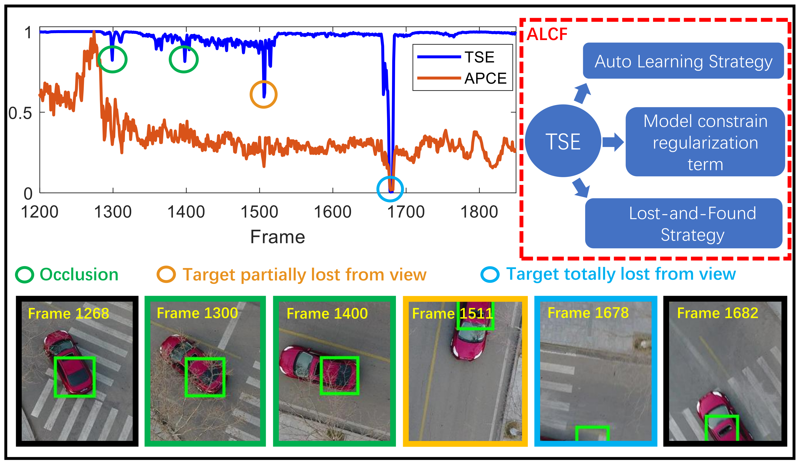
- We present a novel TSE metric to the community which allows accurate estimation of the target state.
- We introduce a new ALCF tracker upon TSE, which consists of a novel auto-learning strategy, a fast lost-and-found strategy, and an effective regularization term for efficient and robust UAV tracking.
- We propose a deep version model which outperforms numerous recently popular deep framework-based trackers and established the new state-of-the-art on several UAV datasets.
- We provide the community with an optimal hand-drafted feature-correlation filter at over 50 FPS on a single CPU.
2. Method
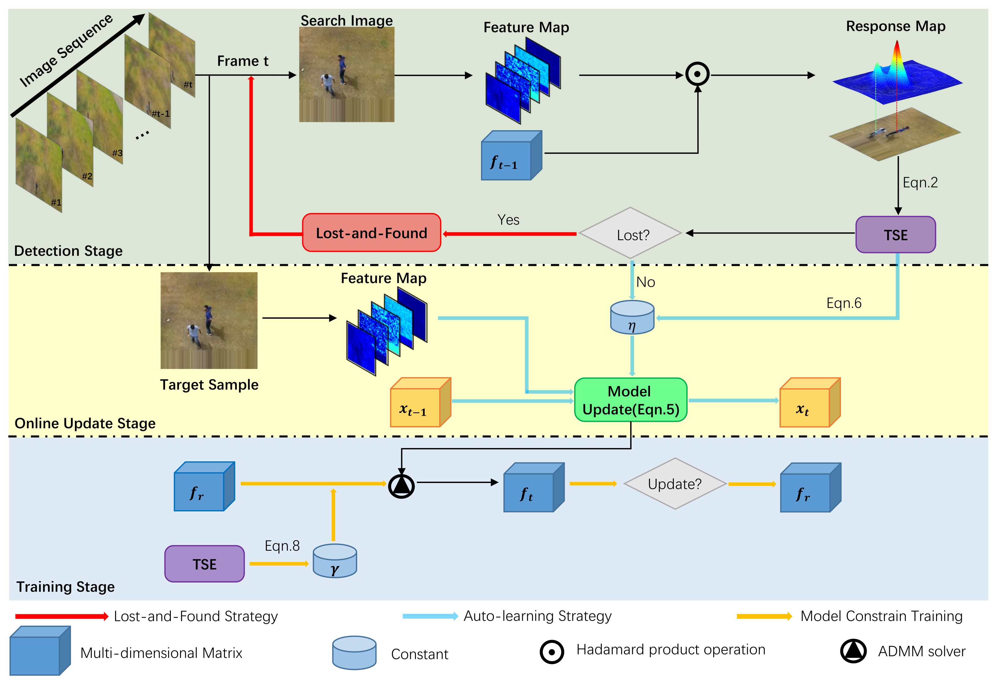
2.1. Overview
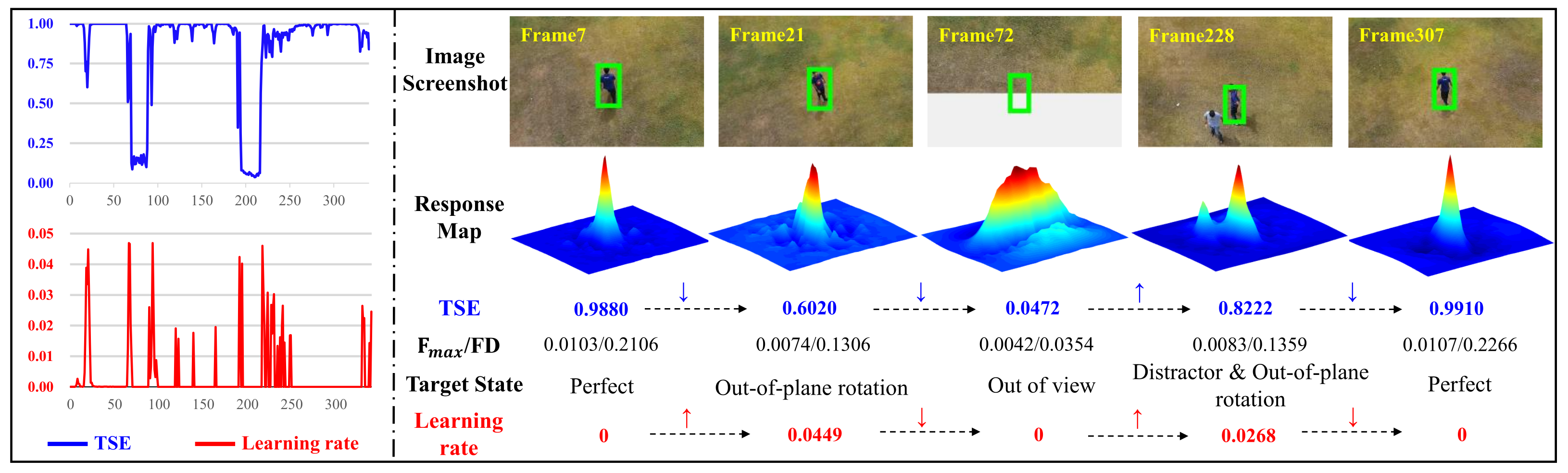
2.2. Target State Estimation (TSE)
2.3. Auto-Learning Correlation Filter
2.3.1. Auto-Learning Strategy
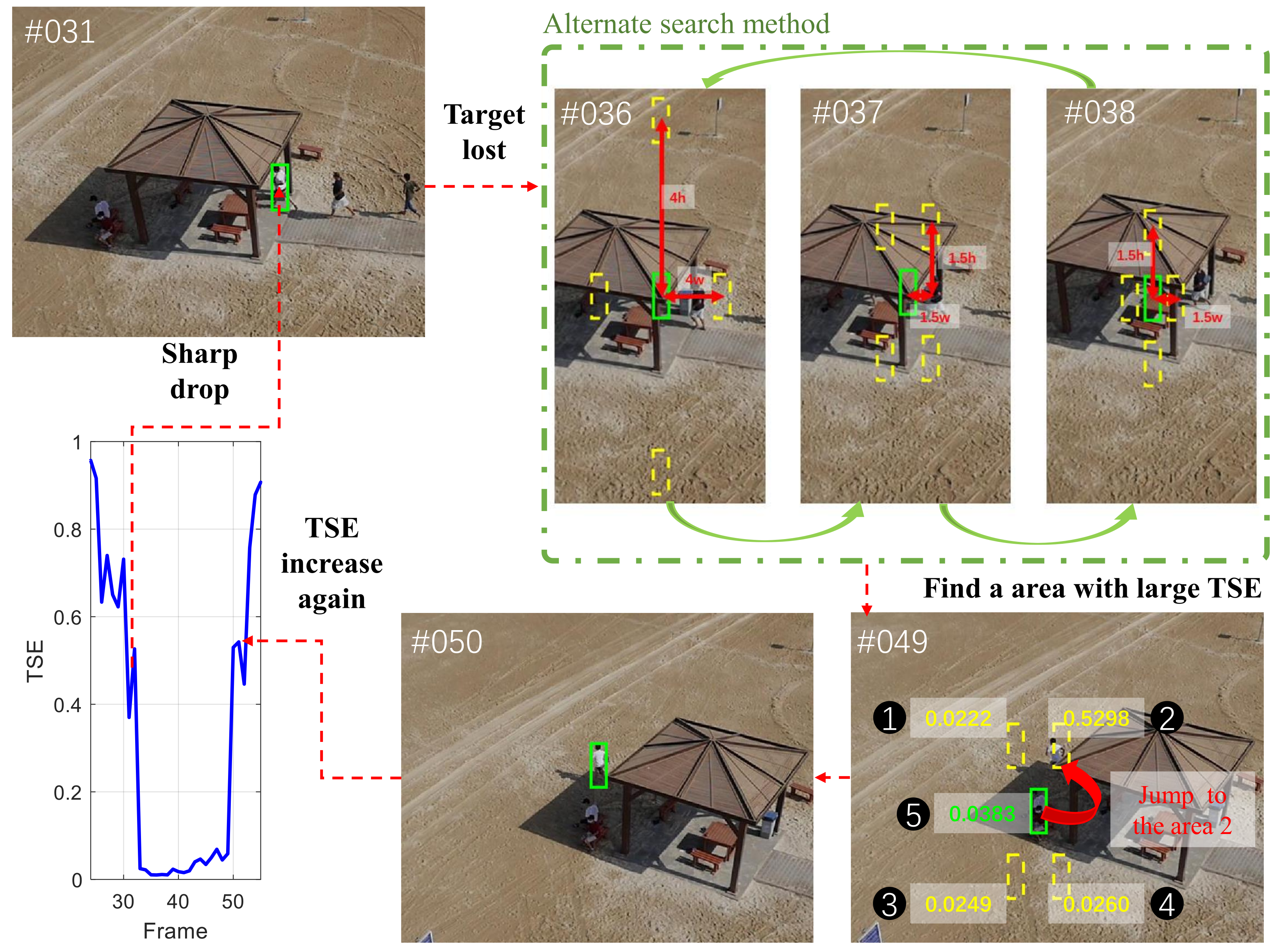
2.3.2. Lost-and-Found Strategy
2.3.3. Model Constrain Regularization
2.4. Model Optimization
2.5. Optimization Solutions
2.5.1. The Solution to Sub-Problem
2.5.2. The Solution to Sub-Problem
2.5.3. Update of Lagrangian Parameter
3. Results and Discussion
3.1. Implementation Details
3.2. Comparison with Hand-Crafted Trackers
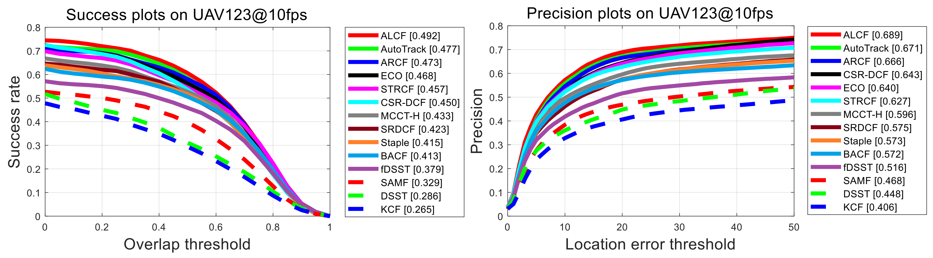
3.2.1. Results on UAV123@10fps
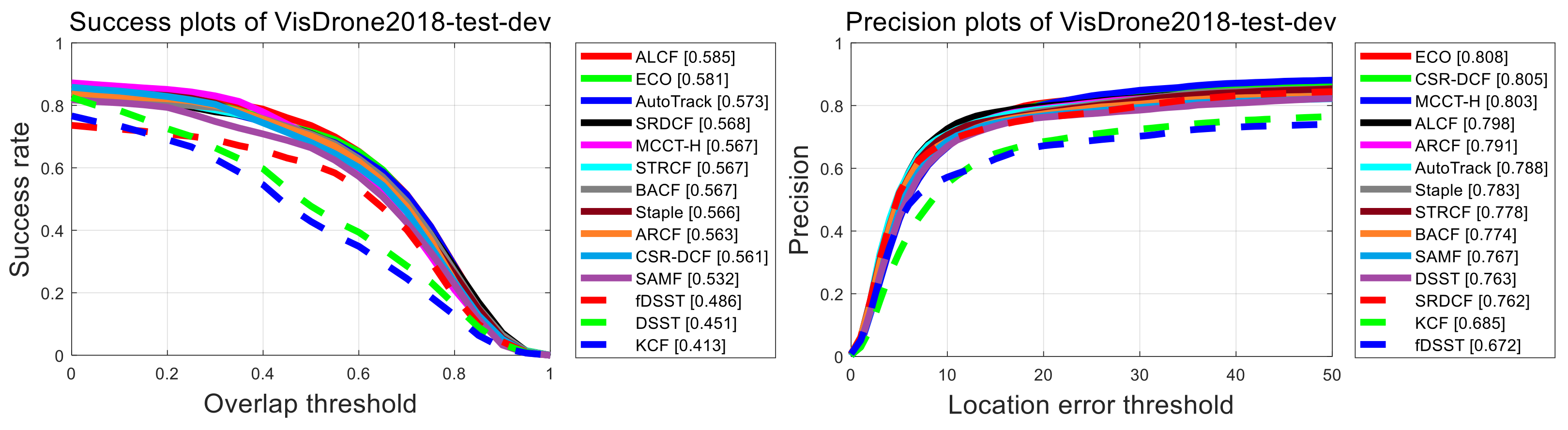
3.2.2. Results on VisDrone2018-Test-Dev
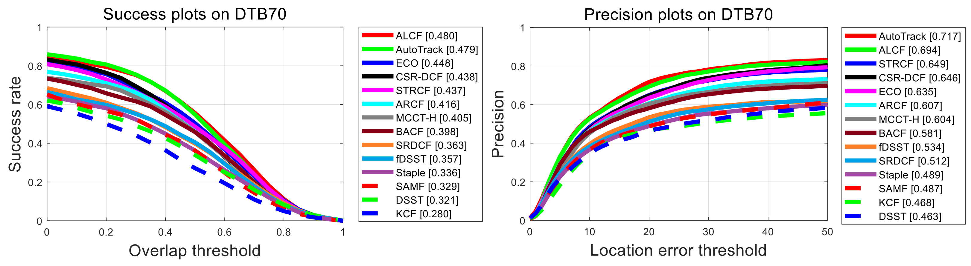
3.2.3. Results on DTB70
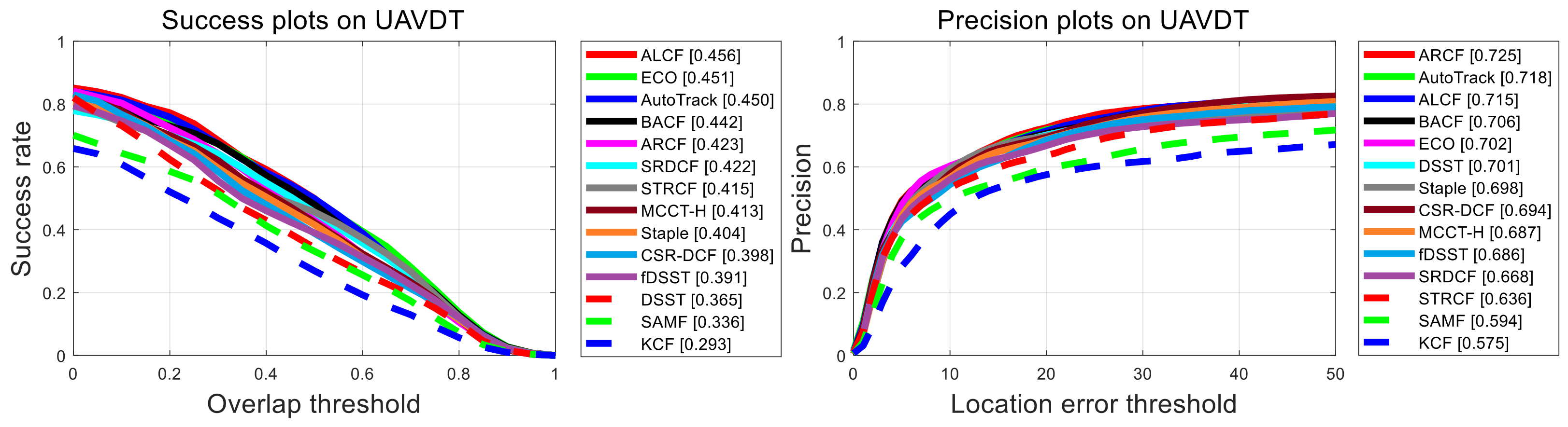
3.2.4. Results on UAVDT
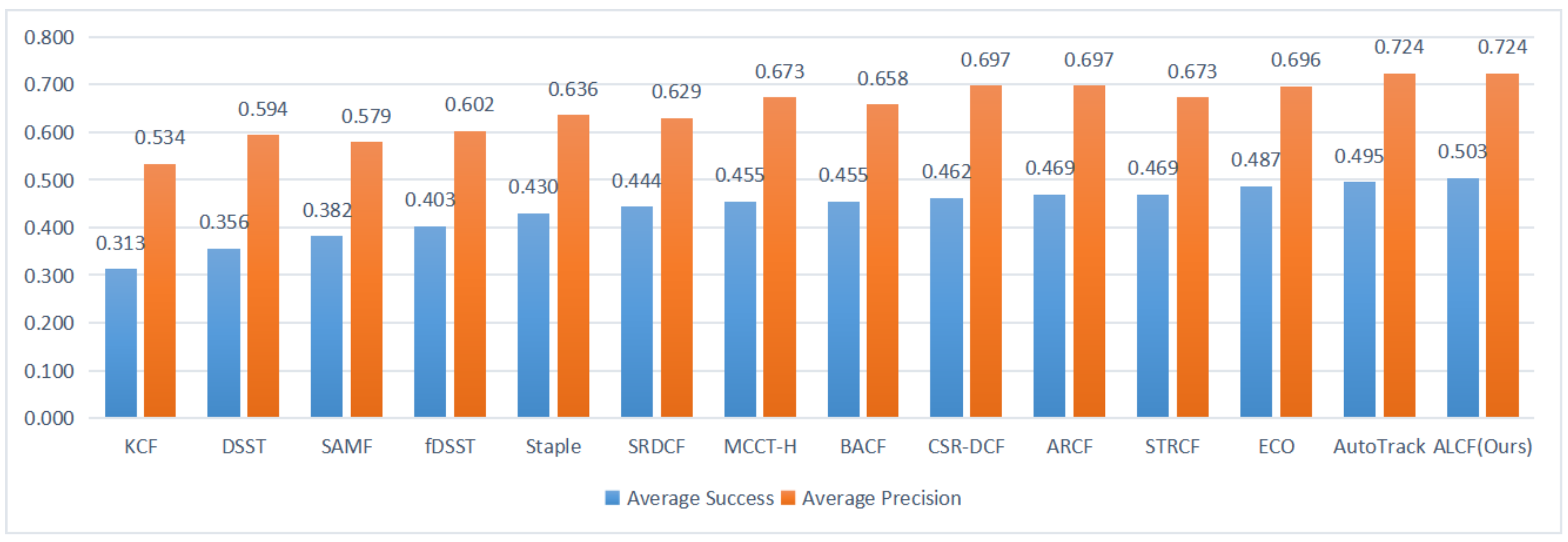
3.2.5. Average Performance Results
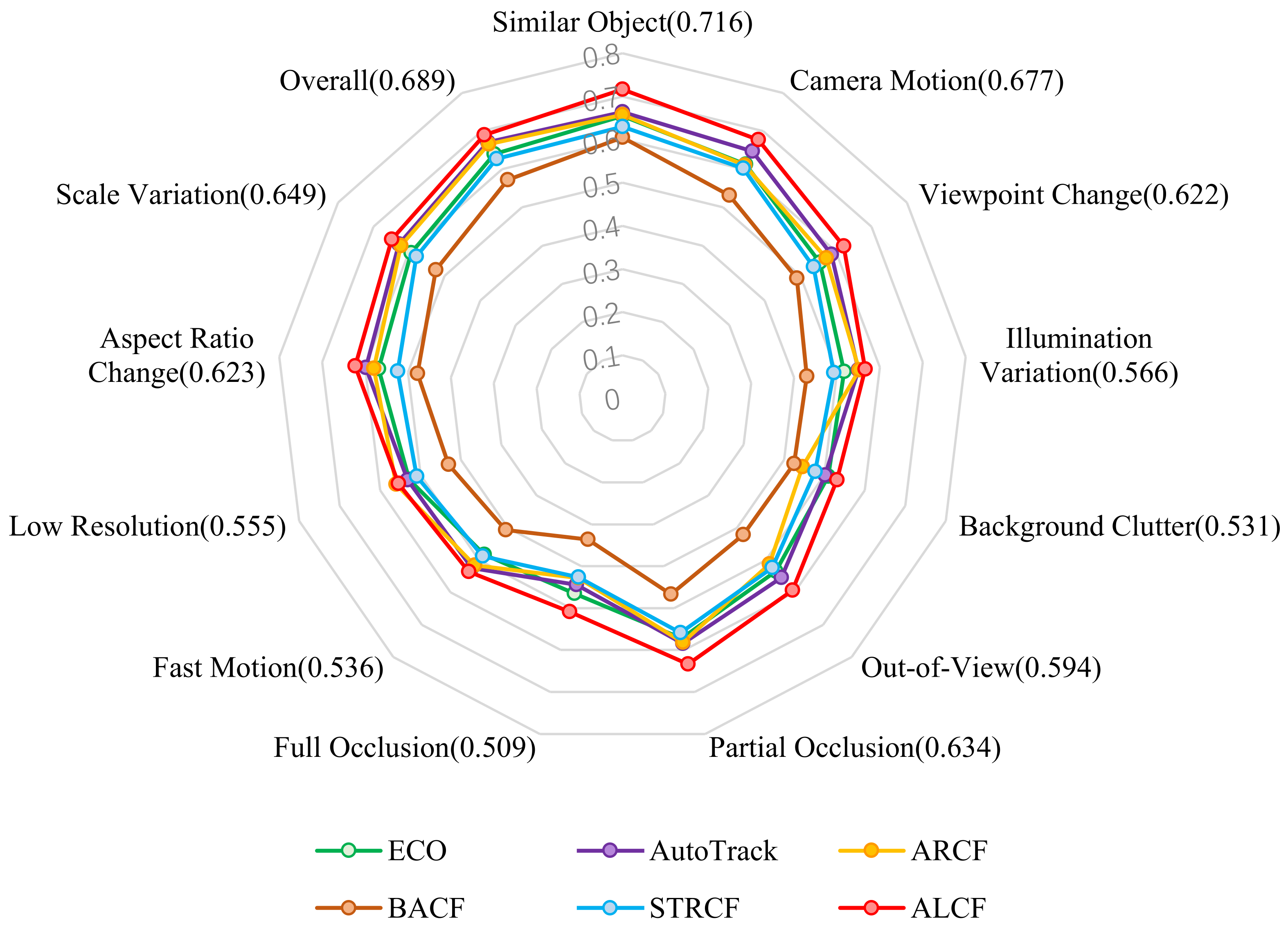
3.2.6. Per-Attribute Evaluation
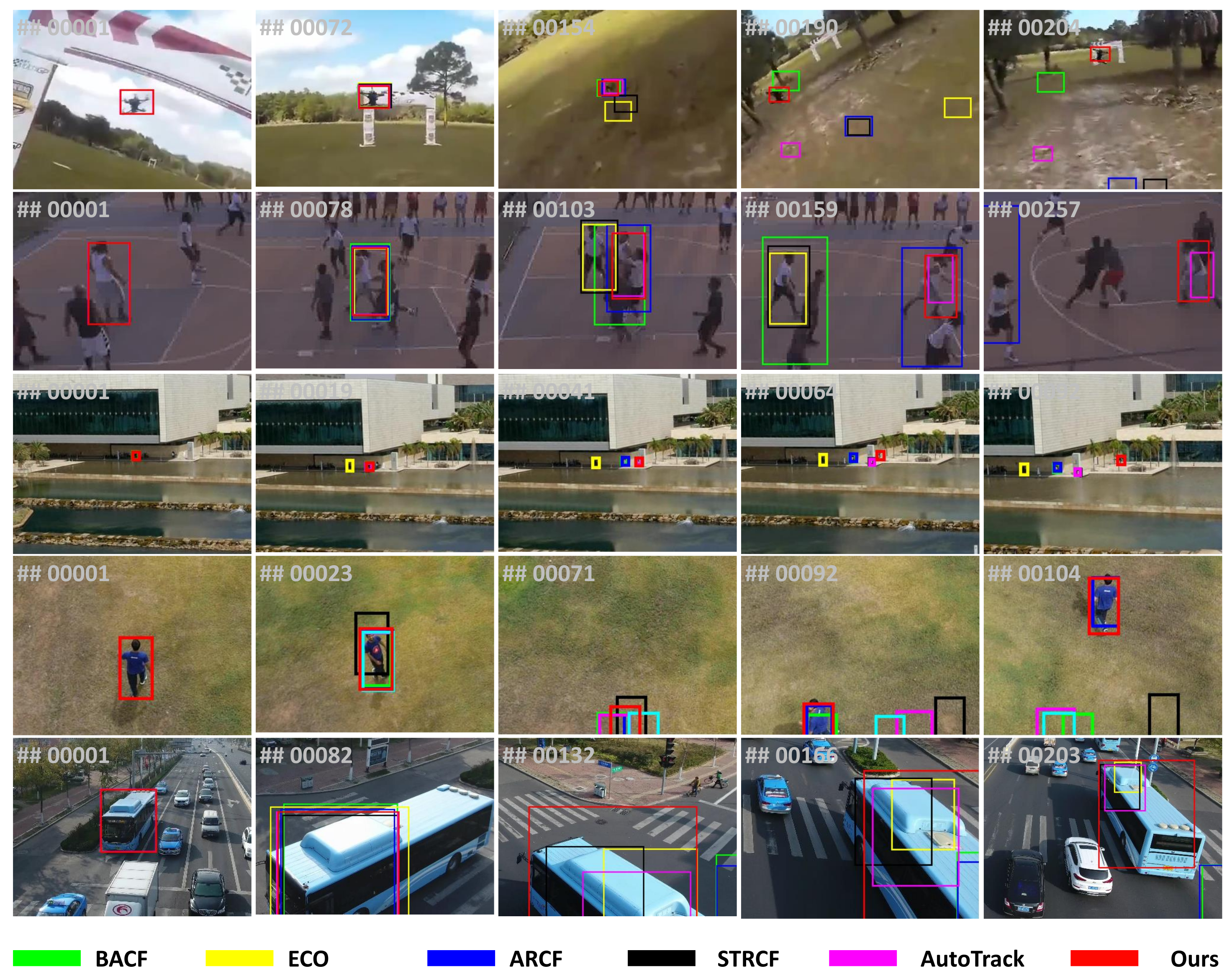
3.2.7. Visualization
3.2.8. Speed
3.3. Ablation Studies
3.3.1. Effect of Auto-Learning Strategy
3.3.2. Effect of Regularization Term
3.3.3. Effect of the Lost-and-Found Strategy
3.3.4. Effect of the Objective Function
3.3.5. Construction of Target State Estimation
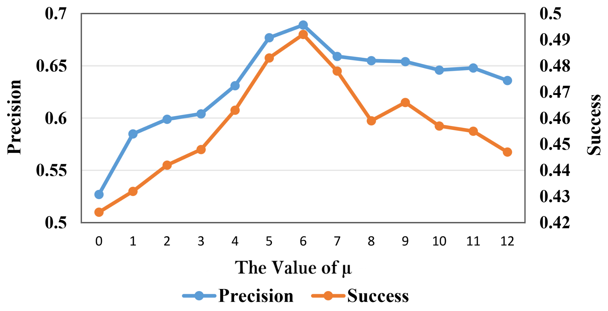
3.3.6. Sensitivity Analysis of Model Constraint Regularization Term
3.4. Extension to Deep Trackers
3.4.1. Results on VisDrone2018-Test-Dev
3.4.2. Results on UAVDT
3.4.3. Results on DTB70
3.4.4. Results on UAV123@10fps
4. Conclusions
Author Contributions
Funding
Institutional Review Board Statement
Informed Consent Statement
Data Availability Statement
Acknowledgments
Conflicts of Interest
References
- Lin, B.; Bai, Y.; Bai, B.; Li, Y. Robust Correlation Tracking for UAV with Feature Integration and Response Map Enhancement. Remote Sens. 2022, 14, 4073. [Google Scholar] [CrossRef]
- Li, Y.; Fu, C.; Ding, F.; Huang, Z.; Lu, G. AutoTrack: Towards High-Performance Visual Tracking for UAV with Automatic Spatio-Temporal Regularization. In Proceedings of the IEEE Conference on Computer Vision and Pattern Recognition, Seattle, WA, USA, 13–19 June 2020; pp. 11923–11932. [Google Scholar]
- Huang, Z.; Fu, C.; Li, Y.; Lin, F.; Lu, P. Learning Aberrance Repressed Correlation Filters for Real-Time UAV Tracking. In Proceedings of the IEEE International Conference on Computer Vision, Seoul, Korea, 27 October–2 November 2019; pp. 2891–2900. [Google Scholar]
- Chen, J.; Xu, T.; Li, J.; Wang, L.; Wang, Y.; Li, X. Adaptive Gaussian-Like Response Correlation Filter for UAV Tracking. In Proceedings of the ICIG, Haikou, China, 6–8 August 2021; pp. 596–609. [Google Scholar]
- Wang, L.; Li, J.; Huang, B.; Chen, J.; Li, X.; Wang, J.; Xu, T. Auto-Perceiving Correlation Filter for UAV Tracking. IEEE Trans. Circuits Syst. Video Technol. 2022, 32, 5748–5761. [Google Scholar] [CrossRef]
- Nex, F.; Remondino, F. UAV for 3D mapping applications: A review. Appl. Geomat. 2014, 6, 1–15. [Google Scholar] [CrossRef]
- Torresan, C.; Berton, A.; Carotenuto, F.; Gennaro, S.F.D.; Gioli, B.; Matese, A.; Miglietta, F.; Vagnoli, C.; Zaldei, A.; Wallace, L. Forestry applications of UAVs in Europe: A review. Int. J. Remote Sens. 2017, 38, 2427–2447. [Google Scholar] [CrossRef]
- Karaduman, M.; Cınar, A.; Eren, H. UAV Traffic Patrolling via Road Detection and Tracking in Anonymous Aerial Video Frames. J. Intell. Robot. Syst. 2019, 95, 675–690. [Google Scholar] [CrossRef]
- Huang, B.; Chen, J.; Xu, T.; Wang, Y.; Jiang, S.; Wang, Y.; Wang, L.; Li, J. SiamSTA: Spatio-Temporal Attention based Siamese Tracker for Tracking UAVs. In Proceedings of the 2021 IEEE/CVF International Conference on Computer Vision Workshops (ICCVW), Montreal, BC, Canada, 11–17 October 2021; pp. 1204–1212. [Google Scholar]
- Lukežič, A.; Vojíř, T.; Čehovin Zajc, L.; Matas, J.; Kristan, M. Discriminative Correlation Filter with Channel and Spatial Reliability. In Proceedings of the IEEE Conference on Computer Vision and Pattern Recognition, Honolulu, HI, USA, 21–26 July 2017; pp. 6309–6318. [Google Scholar]
- Danelljan, M.; Häger, G.; Khan, F.S.; Felsberg, M. Discriminative Scale Space Tracker. IEEE Trans. Pattern Anal. Mach. Intell. 2017, 39, 1561–1575. [Google Scholar] [CrossRef] [PubMed]
- Danelljan, M.; Häger, G.; Khan, F.; Felsberg, M. Learning Spatially Regularized Correlation Filters for Visual Tracking. In Proceedings of the IEEE International Conference on Computer Vision, Santiago, Chile, 7–13 December 2015; pp. 4310–4318. [Google Scholar]
- Galoogahi, H.K.; Fagg, A.; Lucey, S. Learning Background-Aware Correlation Filters for Visual Tracking. In Proceedings of the IEEE International Conference on Computer Vision, Venice, Italy, 22–29 October 2017; pp. 1144–1152. [Google Scholar]
- Huang, B.; Xu, T.; Jiang, S.; Chen, Y.; Bai, Y. Robust visual tracking via constrained multi-kernel correlation filters. IEEE Trans. Multimed. 2020, 22, 2820–2832. [Google Scholar] [CrossRef]
- Wang, N.; Song, Y.; Ma, C.; Zhou, W.; Liu, W.; Li, H. Unsupervised Deep Tracking. In Proceedings of the IEEE Conference on Computer Vision and Pattern Recognition, Long Beach, CA, USA, 15–20 June 2019; pp. 1308–1317. [Google Scholar]
- Nam, H.; Han, B. Learning Multi-Domain Convolutional Neural Networks for Visual Tracking. In Proceedings of the IEEE Conference on Computer Vision and Pattern Recognition, Las Vegas, NV, USA, 27–30 June 2016; pp. 4293–4302. [Google Scholar]
- Li, B.; Yan, J.; Wu, W.; Zhu, Z.; Hu, X. High Performance Visual Tracking With Siamese Region Proposal Network. In Proceedings of the IEEE Conference on Computer Vision and Pattern Recognition, Salt Lake City, UT, USA, 18–23 June 2018; pp. 8971–8980. [Google Scholar]
- Wang, Y.; Xu, T.; Jiang, S.; Chen, J.; Li, J. Pyramid Correlation based Deep Hough Voting for Visual Object Tracking. In Proceedings of the Asian Conference on Machine Learning, PMLR, Virtual Event, 17–19 November 2021; pp. 610–625. [Google Scholar]
- Wang, M.; Liu, Y.; Huang, Z. Large margin object tracking with circulant feature maps. In Proceedings of the IEEE Conference on Computer Vision and Pattern Recognition, Honolulu, HI, USA, 21–26 July 2017; pp. 4021–4029. [Google Scholar]
- Danelljan, M.; Bhat, G.; Khan, F.S.; Felsberg, M. ATOM: Accurate Tracking by Overlap Maximization. In Proceedings of the IEEE Conference on Computer Vision and Pattern Recognition, Long Beach, CA, USA, 16–20 June 2019; pp. 4660–4669. [Google Scholar]
- Zhu, Z.; Wang, Q.; Li, B.; Wu, W.; Yan, J.; Hu, W. Distractor-Aware Siamese Networks for Visual Object Tracking. In Proceedings of the European Conference on Computer Vision, Munich, Germany, 8–14 September 2018; pp. 101–117. [Google Scholar]
- Bolme, D.; Beveridge, J.; Draper, B.; Lui, Y.M. Visual object tracking using adaptive correlation filters. In Proceedings of the IEEE Conference on Computer Vision and Pattern Recognition, San Francisco, CA, USA, 13–18 June 2010; pp. 2544–2550. [Google Scholar]
- Henriques, J.F.; Caseiro, R.; Martins, P.; Batista, J.P. Exploiting the Circulant Structure of Tracking-by-Detection with Kernels. In Proceedings of the European Conference on Computer Vision, Florence, Italy, 7–13 October 2012; Springer: Berlin/Heidelberg, Germany, 2012; pp. 702–715. [Google Scholar]
- Dai, K.; Wang, D.; Lu, H.; Sun, C.; Li, J. Visual Tracking via Adaptive Spatially-Regularized Correlation Filters. In Proceedings of the IEEE Conference on Computer Vision and Pattern Recognition, Long Beach, CA, USA, 16–20 June 2019; pp. 4670–4679. [Google Scholar]
- Xu, T.; Feng, Z.; Wu, X.J.; Kittler, J. Adaptive Channel Selection for Robust Visual Object Tracking with Discriminative Correlation Filters. Int. J. Comput. Vis. 2021, 129, 1359–1375. [Google Scholar] [CrossRef]
- Wang, F.; Yin, S.; Mbelwa, J.T.; Sun, F. Context and saliency aware correlation filter for visual tracking. Multimed. Tools Appl. 2022, 81, 27879–27893. [Google Scholar] [CrossRef]
- Fu, C.; Xu, J.; Lin, F.; Guo, F.; Liu, T.; Zhang, Z. Object Saliency-Aware Dual Regularized Correlation Filter for Real-Time Aerial Tracking. IEEE Trans. Geosci. Remote Sens. 2020, 58, 8940–8951. [Google Scholar] [CrossRef]
- Li, F.; Tian, C.; Zuo, W.; Zhang, L.; Yang, M.H. Learning Spatial-Temporal Regularized Correlation Filters for Visual Tracking. In Proceedings of the IEEE Conference on Computer Vision and Pattern Recognition, Salt Lake City, UT, USA, 18–22 June 2018; pp. 4904–4913. [Google Scholar]
- Huang, B.; Xu, T.; Shen, Z.; Jiang, S.; Zhao, B.; Bian, Z. SiamATL: Online Update of Siamese Tracking Network via Attentional Transfer Learning. IEEE Trans. Cybern. 2021, 52, 7527–7540. [Google Scholar] [CrossRef] [PubMed]
- Dai, K.; Zhang, Y.; Wang, D.; Li, J.; Lu, H.; Yang, X. High-performance long-term tracking with meta-updater. In Proceedings of the IEEE/CVF Conference on Computer Vision and Pattern Recognition, Seattle, WA, USA, 13–19 June 2020; pp. 6298–6307. [Google Scholar]
- Yang, T.; Xu, P.; Hu, R.; Chai, H.; Chan, A.B. ROAM: Recurrently optimizing tracking model. In Proceedings of the IEEE/CVF Conference on Computer Vision and Pattern Recognition, Seattle, WA, USA, 13–19 June 2020; pp. 6718–6727. [Google Scholar]
- Xingjian, S.; Chen, Z.; Wang, H.; Yeung, D.Y.; Wong, W.K.; Woo, W.c. Convolutional LSTM network: A machine learning approach for precipitation nowcasting. In Proceedings of the Advances in Neural Information Processing Systems, Montreal, QC, Canada, 7–12 December 2015; pp. 802–810. [Google Scholar]
- Chen, J.; Xu, T.; Huang, B.; Wang, Y.; Li, J. ARTracker: Compute a More Accurate and Robust Correlation Filter for UAV Tracking. IEEE Geosci. Remote Sens. Lett. 2022, 19, 1–5. [Google Scholar] [CrossRef]
- Kalal, Z.; Mikolajczyk, K.; Matas, J. Tracking-Learning-Detection. IEEE Trans. Softw. Eng. 2011, 34, 1409–1422. [Google Scholar] [CrossRef]
- Fan, H.; Ling, H. Parallel Tracking and Verifying: A Framework for Real-Time and High Accuracy Visual Tracking. In Proceedings of the IEEE International Conference on Computer Vision, Venice, Italy, 22–29 October 2017; pp. 5487–5495. [Google Scholar]
- Lukezic, A.; Zajc, L.C.; Vojír, T.; Matas, J.; Kristan, M. FCLT-A Fully-Correlational Long-Term Tracker. arXiv 2018, arXiv:1804.07056. [Google Scholar]
- Voigtlaender, P.; Luiten, J.; Torr, P.H.; Leibe, B. Siam R-CNN: Visual Tracking by Re-Detection. In Proceedings of the IEEE Conference on Computer Vision and Pattern Recognition, Seattle, WA, USA, 13–19 June 2020; pp. 6578–6588. [Google Scholar]
- Huang, L.; Zhao, X.; Huang, K. GlobalTrack: A Simple and Strong Baseline for Long-Term Tracking. In Proceedings of the AAAI Conference on Artificial Intelligence, New York, NY, USA, 7–12 February 2020; Volume 34, pp. 11037–11044. [Google Scholar]
- Du, D.; Qi, Y.; Yu, H.; Yang, Y.; Duan, K.; Li, G.; Zhang, W.; Huang, Q.; Tian, Q. The Unmanned Aerial Vehicle Benchmark: Object Detection and Tracking. In Proceedings of the European conference on computer vision (ECCV), Munich, Germany, 8–14 September 2018; pp. 370–386. [Google Scholar]
- Müller, M.; Smith, N.; Ghanem, B. A Benchmark and Simulator for UAV Tracking. In Proceedings of the European Conference on Computer Vision, Amsterdam, The Netherlands, 11–14 October 2016; Springer: Berlin/Heidelberg, Germany, 2016; pp. 445–461. [Google Scholar]
- Li, S.; Yeung, D.Y. Visual object tracking for unmanned aerial vehicles: A benchmark and new motion models. In Proceedings of the AAAI Conference on Artificial Intelligence, San Francisco, CA, USA, 4–9 February 2017; Volume 31. [Google Scholar]
- Zhu, P.; Wen, L.; Bian, X.; Ling, H.; Hu, Q. Vision Meets Drones: A Challenge. In Proceedings of the European Conference on Computer Vision, Munich, Germany, 8–14 September 2018; Springer: Berlin/Heidelberg, Germany, 2018. [Google Scholar]
- Danelljan, M.; Häger, G.; Khan, F.; Felsberg, M. Accurate scale estimation for robust visual tracking. In Proceedings of the British Machine Vision Conference, Nottingham, UK, 1–5 September 2014; Bmva Press: Newcastle, UK, 2014. [Google Scholar]
- Yan, B.; Zhang, X.; Wang, D.; Lu, H.; Yang, X. Alpha-refine: Boosting tracking performance by precise bounding box estimation. In Proceedings of the CVPR, Virtual, 19–25 June 2021; pp. 5289–5298. [Google Scholar]
- Galoogahi, H.K.; Sim, T.; Lucey, S. Multi-channel Correlation Filters. In Proceedings of the IEEE International Conference on Computer Vision, Sydney, Australia, 1–8 December 2013; pp. 3072–3079. [Google Scholar]
- Sherman, J.; Morrison, W.J. Adjustment of an Inverse Matrix Corresponding to a Change in One Element of a Given Matrix. Ann. Math. Stat. 1950, 21, 124–127. [Google Scholar] [CrossRef]
- Dalal, N.; Triggs, B. Histograms of oriented gradients for human detection. In Proceedings of the 2005 IEEE Computer Society Conference on Computer Vision and Pattern Recognition (CVPR’05), San Diego, CA, USA, 20–26 June 2005; Volume 1, pp. 886–893. [Google Scholar]
- Danelljan, M.; Khan, F.; Felsberg, M.; van de Weijer, J. Adaptive Color Attributes for Real-Time Visual Tracking. In Proceedings of the IEEE Conference on Computer Vision and Pattern Recognition, Columbus, OH, USA, 23–28 June 2014; pp. 1090–1097. [Google Scholar]
- Danelljan, M.; Bhat, G.; Shahbaz Khan, F.; Felsberg, M. ECO: Efficient Convolution Operators for Tracking. In Proceedings of the IEEE Conference on Computer Vision and Pattern Recognition, Honolulu, HI, USA, 21–26 July 2017; pp. 6638–6646. [Google Scholar]
- Wang, N.; Zhou, W.; Tian, Q.; Hong, R.; Wang, M.; Li, H. Multi-cue Correlation Filters for Robust Visual Tracking. In Proceedings of the IEEE Conference on Computer Vision and Pattern Recognition, Salt Lake City, UT, USA, 18–22 June 2018; pp. 4844–4853. [Google Scholar]
- Bertinetto, L.; Valmadre, J.; Golodetz, S.; Miksik, O.; Torr, P.H.S. Staple: Complementary Learners for Real-Time Tracking. In Proceedings of the IEEE Conference on Computer Vision and Pattern Recognition, Las Vegas, NV, USA, 27–30 June 2016; pp. 1401–1409. [Google Scholar]
- Li, Y.; Zhu, J. A Scale Adaptive Kernel Correlation Filter Tracker with Feature Integration. In Proceedings of the European Conference on Computer Vision, Zurich, Switzerland, 5–12 September 2014; pp. 254–265. [Google Scholar]
- Henriques, J.F.; Caseiro, R.; Martins, P.; Batista, J. High-Speed Tracking with Kernelized Correlation Filters. IEEE Trans. Pattern Anal. Mach. Intell. 2015, 37, 583–596. [Google Scholar] [CrossRef]
- Bhat, G.; Danelljan, M.; Gool, L.V.; Timofte, R. Know your surroundings: Exploiting scene information for object tracking. In European Conference on Computer Vision; Springer: Cham, Switzerland, 2020; pp. 205–221. [Google Scholar]
- Bhat, G.; Danelljan, M.; Gool, L.V.; Timofte, R. Learning Discriminative Model Prediction for Tracking. In Proceedings of the IEEE International Conference on Computer Vision, Seoul, Korea, 27 October–2 November 2019; pp. 6182–6191. [Google Scholar]
- Danelljan, M.; Bhat, G. PyTracking: Visual Tracking Library Based on PyTorch. Available online: https://github.com/visionml/pytracking (accessed on 8 January 2020).
- Danelljan, M.; Gool, L.V.; Timofte, R. Probabilistic Regression for Visual Tracking. In Proceedings of the IEEE Conference on Computer Vision and Pattern Recognition, Seattle, WA, USA, 13–19 June 2020; pp. 7183–7192. [Google Scholar]
- Valmadre, J.; Bertinetto, L.; Henriques, J.; Vedaldi, A.; Torr, P.H.S. End-To-End Representation Learning for Correlation Filter Based Tracking. In Proceedings of the IEEE Conference on Computer Vision and Pattern Recognition, Honolulu, HI, USA, 21–26 July 2017; pp. 2805–2813. [Google Scholar]
- Cao, Z.; Fu, C.; Ye, J.; Li, B.; Li, Y. HiFT: Hierarchical Feature Transformer for Aerial Tracking. In Proceedings of the IEEE/CVF International Conference on Computer Vision, Montreal, QC, Canada, 10–17 October 2021; pp. 15457–15466. [Google Scholar]
- Li, X.; Ma, C.; Wu, B.; He, Z.; Yang, M.H. Target-Aware Deep Tracking. In Proceedings of the IEEE Conference on Computer Vision and Pattern Recognition, Long Beach, CA, USA, 16–20 June 2019; pp. 1369–1378. [Google Scholar]
- Wang, N.; Zhou, W.; Song, Y.; Ma, C.; Li, H. Real-time correlation tracking via joint model compression and transfer. IEEE Trans. Image Process. 2020, 29, 6123–6135. [Google Scholar] [CrossRef]
- Wang, N.; Zhou, W.; Song, Y.; Ma, C.; Liu, W.; Li, H. Unsupervised deep representation learning for real-time tracking. Int. J. Comput. Vis. 2021, 129, 400–418. [Google Scholar] [CrossRef]
- Ma, C.; Huang, J.B.; Yang, X.; Yang, M.H. Hierarchical Convolutional Features for Visual Tracking. In Proceedings of the IEEE International Conference on Computer Vision, Santiago, Chile, 7–13 December 2015; pp. 3074–3082. [Google Scholar]
- Li, F.; Yao, Y.; Li, P.; Zhang, D.; Zuo, W.; Yang, M.H. Integrating Boundary and Center Correlation Filters for Visual Tracking with Aspect Ratio Variation. In Proceedings of the IEEE International Conference on Computer Orkshops (ICCVW), Venice, Italy, 22–29 October 2017; pp. 2001–2009. [Google Scholar]
- Song, Y.; Ma, C.; Gong, L.; Zhang, J.; Lau, R.; Yang, M.H. CREST: Convolutional Residual Learning for Visual Tracking. In Proceedings of the IEEE International Conference on Computer Vision, Venice, Italy, 22–29 October 2017; pp. 2555–2564. [Google Scholar]
- Yun, S.; Choi, J.; Yoo, Y.; Yun, K.; Young Choi, J. Action-decision networks for visual tracking with deep reinforcement learning. In Proceedings of the CVPR, Honolulu, HI, USA, 21–28 July 2017; pp. 2711–2720. [Google Scholar]
- Li, Y.; Fu, C.; Huang, Z.; Zhang, Y.; Pan, J. Intermittent contextual learning for keyfilter-aware uav object tracking using deep convolutional feature. IEEE Trans. Multimed. 2020, 23, 810–822. [Google Scholar] [CrossRef]
- Bertinetto, L.; Valmadre, J.; Henriques, J.F.; Vedaldi, A.; Torr, P.H.S. Fully-Convolutional Siamese Networks for Object Tracking. In European Conference on Computer Vision; Springer: Cham, Switzerland, 2016; pp. 850–865. [Google Scholar]
- Danelljan, M.; Robinson, A.; Khan, F.; Felsberg, M. Beyond Correlation Filters: Learning Continuous Convolution Operators for Visual Tracking. In European Conference on Computer Vision; Springer: Cham, Switzerland, 2016; pp. 472–488. [Google Scholar]


| ALCF | AutoTrack | ECO-HC | STRCF-HC | ARCF | |
|---|---|---|---|---|---|
| FPS | 51.3 | 58.3 | 69.4 | 23.2 | 23.3 |
| Success | 0.503 | 0.494 | 0.487 | 0.469 | 0.469 |
| Precision | 0.724 | 0.723 | 0.696 | 0.672 | 0.697 |
| AL | MC | LF | R | Precision | AUC | FPS | |
|---|---|---|---|---|---|---|---|
| Baseline | 0.600 | 0.432 | 36.94 | ||||
| ✓ | 0.637 | 0.460 | 45.64 | ||||
| ✓ | 0.649 | 0.463 | 34.03 | ||||
| ✓ | 0.648 | 0.465 | 32.38 | ||||
| ✓ | ✓ | 0.654 | 0.468 | 32.36 | |||
| ✓ | ✓ | ✓ | 0.667 | 0.473 | 47.89 | ||
| ✓ | ✓ | 0.654 | 0.469 | 42.44 | |||
| ✓ | ✓ | 0.650 | 0.464 | 33.70 | |||
| ✓ | ✓ | 0.652 | 0.474 | 36.52 | |||
| ✓ | ✓ | ✓ | 0.662 | 0.475 | 29.91 | ||
| ✓ | ✓ | ✓ | ✓ | 0.689 | 0.492 | 41.31 | |
| Baseline+STRCF | 0.638 | 0.457 | 31.87 | ||||
| Baseline+MC+Fix | 0.639 | 0.459 | 33.40 |
| MDNet [16] | UDT+ [15] | PrDiMP [57] | ATOM [20] | DiMP [55] | SiamRPN [17] | CFNet [58] | Super_DiMP [56] | KYS [54] | HiFT [59] | ALCF Ours | DeepALCF Ours | |
|---|---|---|---|---|---|---|---|---|---|---|---|---|
| Precision | 0.790 | 0.800 | 0.797 | 0.751 | 0.806 | 0.781 | 0.778 | 0.800 | 0.810 | 0.721 | 0.798 | 0.816 |
| Success | 0.579 | 0.584 | 0.600 | 0.563 | 0.605 | 0.573 | 0.568 | 0.610 | 0.600 | 0.527 | 0.585 | 0.619 |
| Trackers | Venue | Precision | Success |
|---|---|---|---|
| MDNet [16] | CVPR2016 | 0.725 | 0.464 |
| MCCT [50] | CVPR2018 | 0.691 | 0.448 |
| ASRCF [24] | CVPR2019 | 0.720 | 0.449 |
| TADT [60] | CVPR2019 | 0.700 | 0.441 |
| UDT [15] | CVPR2019 | 0.674 | 0.442 |
| UDT+ [15] | CVPR2020 | 0.696 | 0.415 |
| PrDiMP [57] | CVPR2020 | 0.757 | 0.559 |
| fECO [61] | TIP2020 | 0.699 | 0.415 |
| fDSTRCF [61] | TIP2020 | 0.677 | 0.454 |
| HiFT [59] | ICCV2021 | 0.652 | 0.474 |
| LUDT [62] | IJCV2021 | 0.631 | 0.418 |
| LUDT+ [62] | IJCV2021 | 0.701 | 0.406 |
| ALCF | Ours | 0.725 | 0.456 |
| DeepALCF | Ours | 0.748 | 0.534 |
| Trackers | Venue | Precision | Success |
|---|---|---|---|
| HCF [63] | ICCV2015 | 0.616 | 0.415 |
| MDNet [16] | CVPR2016 | 0.703 | 0.466 |
| CFNet [58] | CVPR2017 | 0.587 | 0.398 |
| IBCCF [64] | ICCVW2017 | 0.669 | 0.460 |
| CREST [65] | ICCV2017 | 0.650 | 0.452 |
| ADNet [66] | CVPR2017 | 0.637 | 0.422 |
| DaSiamRPN [21] | ECCV2018 | 0.735 | 0.512 |
| UDT+ [15] | CVPR2019 | 0.650 | 0.457 |
| MCCT [50] | CVPR2019 | 0.725 | 0.484 |
| TADT [60] | CVPR2019 | 0.690 | 0.460 |
| ASRCF [24] | CVPR2019 | 0.696 | 0.468 |
| KAOT [67] | TMM2020 | 0.692 | 0.469 |
| ARTracker [33] | GRSL2022 | 0.752 | 0.588 |
| ALCF | Ours | 0.694 | 0.480 |
| DeepALCF | Ours | 0.727 | 0.530 |
| Trackers | Precision | Success | Trackers | Precision | Success |
|---|---|---|---|---|---|
| HCF | 0.601 | 0.426 | MDNet | 0.664 | 0.477 |
| CFNet | 0.568 | 0.422 | IBCCF | 0.651 | 0.481 |
| SiamFC [68] | 0.678 | 0.472 | CREST | 0.600 | 0.445 |
| C-COT [69] | 0.704 | 0.502 | DeepSTRCF | 0.680 | 0.499 |
| DaSiamRPN | 0.689 | 0.481 | UDT+ | 0.674 | 0.470 |
| MCCT | 0.689 | 0.496 | ADNet | 0.647 | 0.422 |
| TADT | 0.685 | 0.507 | ASRCF | 0.685 | 0.477 |
| ALCF | 0.689 | 0.492 | DeepALCF | 0.712 | 0.516 |
Publisher’s Note: MDPI stays neutral with regard to jurisdictional claims in published maps and institutional affiliations. |
© 2022 by the authors. Licensee MDPI, Basel, Switzerland. This article is an open access article distributed under the terms and conditions of the Creative Commons Attribution (CC BY) license (https://creativecommons.org/licenses/by/4.0/).
Share and Cite
Bian, Z.; Xu, T.; Chen, J.; Ma, L.; Cai, W.; Li, J. Auto-Learning Correlation-Filter-Based Target State Estimation for Real-Time UAV Tracking. Remote Sens. 2022, 14, 5299. https://doi.org/10.3390/rs14215299
Bian Z, Xu T, Chen J, Ma L, Cai W, Li J. Auto-Learning Correlation-Filter-Based Target State Estimation for Real-Time UAV Tracking. Remote Sensing. 2022; 14(21):5299. https://doi.org/10.3390/rs14215299
Chicago/Turabian StyleBian, Ziyang, Tingfa Xu, Junjie Chen, Liang Ma, Wenjing Cai, and Jianan Li. 2022. "Auto-Learning Correlation-Filter-Based Target State Estimation for Real-Time UAV Tracking" Remote Sensing 14, no. 21: 5299. https://doi.org/10.3390/rs14215299
APA StyleBian, Z., Xu, T., Chen, J., Ma, L., Cai, W., & Li, J. (2022). Auto-Learning Correlation-Filter-Based Target State Estimation for Real-Time UAV Tracking. Remote Sensing, 14(21), 5299. https://doi.org/10.3390/rs14215299