Abstract
Although deep learning has received extensive attention and achieved excellent performance in various scenarios, it suffers from adversarial examples to some extent. In particular, physical attack poses a greater threat than digital attack. However, existing research has paid less attention to the physical attack of object detection in UAV remote sensing images (RSIs). In this work, we carefully analyze the universal adversarial patch attack for multi-scale objects in the field of remote sensing. There are two challenges faced by an adversarial attack in RSIs. On one hand, the number of objects in remote sensing images is more than that of natural images. Therefore, it is difficult for an adversarial patch to show an adversarial effect on all objects when attacking a detector of RSIs. On the other hand, the wide height range of the photography platform causes the size of objects to vary a great deal, which presents challenges for the generation of universal adversarial perturbation for multi-scale objects. To this end, we propose an adversarial attack method of object detection for remote sensing data. One of the key ideas of the proposed method is the novel optimization of the adversarial patch. We aim to attack as many objects as possible by formulating a joint optimization problem. Furthermore, we raise the scale factor to generate a universal adversarial patch that adapts to multi-scale objects, which ensures that the adversarial patch is valid for multi-scale objects in the real world. Extensive experiments demonstrate the superiority of our method against state-of-the-art methods on YOLO-v3 and YOLO-v5. In addition, we also validate the effectiveness of our method in real-world applications.
1. Introduction
The continuous development of aerial photography technology makes it possible for people to collect numerous high-resolution remote sensing images, which contributes to many important applications in the field of remote sensing [1,2,3]. Some typical applications include classification [4,5], image segmentation [6] and object detection [7,8,9,10,11,12,13,14]. Specifically, object detection, which tries to precisely estimate the class and location of objects contained in each image, is the primary task [15,16,17]. Deep learning models, which learn a hierarchical representation of features, have been widely used and have achieved great success in many fields [18,19,20,21], and have played a significant role in most of the state-of-the-art methods used in RSIs. Moreover, the constant improvement of the structure of deep neural networks brings with it better performance.
Although great success has been achieved through the use of deep learning, several potential security problems should not be neglected. Recent studies found that deep models are extremely vulnerable to adversarial examples, which can be easily generated by adding carefully designed perturbations to clean examples. Szegedy et al. [22] first revealed the fragility of deep neural networks and raised the concept of adversarial examples. Since then, an increasing number of researchers have devoted their work to exploring the security of deep learning algorithms and developing corresponding methods for generating adversarial examples. The proposed adversarial attack methods can be divided into digital attacks and physical attacks based on the domain where the adversarial perturbations are added. Digital attacks directly modify the pixel values of the input images in the digital space. Typical digital attack methods include the Fast Gradient Sign Method (FGSM) [23], Projected Gradient Descent (PGD) [24], DeepFool [25], Universal Adversarial Perturbations (UAP) [26], C&W [27] and Jacobian-based Saliency Map Attacks (JSMA) [28]. However, most of the digital attack methods cannot be applied in the real world, because the perturbation may be easily filtered when performing physical attacks. As for physical attacks, the generated perturbation (e.g., adversarial glass [29], adversarial T-shirt [30] and adversarial patch [31]) is always large, and it can be printed and applied in the physical world. Kurakin et al. [32] first performed experiments to verify that adversarial examples also exist in the real world. Thys et al. [33] and Hu et al. [34] generated adversarial patches to fool person detectors.
In addition to the above-mentioned adversarial attack methods, there are currently some works [35,36,37] focused on adversarial examples in the field of remote sensing. Czaja et al. [38] first generated adversarial examples for classification models in RSIs. They attacked a small domain of one image to lead the model to make incorrect predictions. Xu et al. [39] proposed the generation of universal adversarial examples to realize black-box attacks on different models. Chen et al. [40] designed experiments to attack synthetic aperture radar (SAR) images. Xu et al. [41] indicated that hyperspectral images were also affected by adversarial examples. However, it is more difficult to attack object detection than image classification because the number of bounding boxes may be very large. When the confidence of one bounding box drops, the others may still work, which is why object detectors are hard to attack. Lu et al. [42] designed a scale-adaptive patch to attack object detection for RSIs. They took the confidence loss as the loss function. Furthermore, they only performed digital attacks in their experiments. Du et al. [43] adapted Thys et al.’s method [33] and performed digital and physical attacks on an aerial surveillance model, the first work to demonstrate physical attack in aerial scenes.
To date, some works [37,42,44] have focused on generating adversarial examples for RSIs. However, adversarial attack for RSIs has not yet been fully explored. There are still several limitations of adversarial attacks in RSIs. (1) The majority of the existing methods mainly focus on digital attacks, but they are constrained when applied to the physical attack of object detection. (2) The number of objects in RSIs tends to be much greater than that in images captured on the ground, which can be observed in Figure 1. Therefore, it is difficult for an adversarial patch to show an adversarial effect on all objects when attacking a detector of RSIs. (3) Remote sensing images are obtained by using earth-observing photography platforms and the height of the platform is always at a wide range, which causes the size of the objects to vary. This brings challenges in generating universal adversarial perturbation for multi-scale objects.
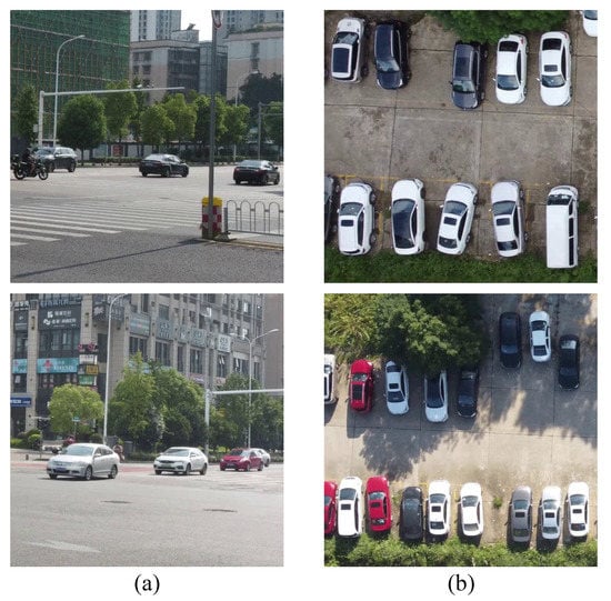
Figure 1.
(a) Images captured on the ground. (b) Remote sensing images. The number of objects in remote sensing images is greater than that in images captured on the ground.
Based on the above analysis, this work aims to conduct adversarial attacks against object detection in digital and physical domains for RSIs. We formulate a joint optimization problem to generate a more effective adversarial patch. In order to attack as many objects as possible, one idea is to take the average confidence as part of the loss, namely object loss. The average confidence is the average value of the confidence of all bounding boxes in a single image, and the computation of average confidence involves all objects for one image, so it is reasonable to believe that more objects will be attacked with the average confidence loss. Considering the fact that the constraint of object loss does not take the detection result into consideration, detection loss between the detection results and the ground truth is also introduced in our method. Thus, we can degrade the metrics (average precision (AP), precision, and recall) by increasing detection loss. The experimental results demonstrate that the attack effect is improved by the combination of the two losses, and relevant theoretical analysis is shown in an ablation study. In consideration of the actual situation, we propose a novel method to match the size of the adversarial patch with the size of the objects in a digital attack, which ensures that the adversarial patch is valid for multi-scale objects. All of the images in our experiments have labels regarding the height of the objects. When carrying out digital attacks, the adversarial patch is scaled to the corresponding size with the scale factor, which depends on the height label of images. Finally, the experimental results show the effectiveness of our method. The contributions of this work can be summarized in the following three points:
- (1)
- To the best of our knowledge, this is the first work to evaluate the attack effect on objects of different scales, and we perform physical adversarial attacks on multi-scale objects. The data from the experiments are captured from 25 m to 120 m by a DJI Mini 2.
- (2)
- For the optimization of the adversarial patch, we formulate a joint optimization problem to generate a more effective adversarial patch. Moreover, to make the generated patch valid for multi-scale objects in the real world, we use a scale factor that depends on the height label of the image to rescale the adversarial patch when performing a digital attack.
- (3)
- To verify the superiority of our method, we carry out several comparison experiments on the digital attack against Yolo-V3 and Yolo-V5. The experimental results demonstrate that our method has a better performance than baseline methods. In addition, we perform experiments to test the effect of our method in the physical world.
The remainder of this paper is organized as follows. Section 2 briefly reviews related attack methods. In Section 3, the details of the proposed method are demonstrated in as much detail as possible. Section 4 provides the experimental results and the corresponding analyses. In Section 5, we draw a comprehensive conclusion.
2. Related Work
2.1. Digital Attack and Physical Attack
An increasing number of researchers have paid attention to the safety of deep learning, ever since Szegedy et al. [22] proposed the concept of the adversarial attack. Currently, the proposed adversarial attack methods can be categorized into digital and physical attacks based on the domain where the adversarial perturbations are added.
Digital attack. The premier studies [22,23,24,25,26,27,28] on adversarial attacks mainly focus on digital attack, in which a tiny perturbation is added to the original input images to make the target model output incorrect predictions. Szegedy et al. [22] proposed Limited Memory Broyden–Fletcher–Goldfarb–Shanno (L-BFGS) to generate adversarial examples for the first time. Based on the gradient information, the Fast Gradient Sign Method (FGSM) [23] proposed by Goodfellow et al. aimed to quickly find an adversarial example for a given input. Madry et al. [24] proposed Projected Gradient Descent (PGD), a first-order attack. DeepFool [25] is another typical attack algorithm that estimates the distance of an input to the closest decision boundary, and it has successfully been used to attack many models. Carlini and Wagner proposed C&W [27] to find adversarial perturbations by minimizing similarity metrics: , , and . Chow et al. [45] presented Targeted Adversarial Objectness (TOG) to cause object detection to suffer from object-vanishing, object-fabrication and object mislabeling attacks. Liu et al. [46] proposed DPatch, adding an adversarial patch to the images to stop detectors from detecting objects. Although these attack methods have achieved great success in the digital domain, their effectiveness is significantly diminished when applied in the real world.
Physical attack. Compared with a digital attack, a physical adversarial attack poses a greater threat in specific scenarios. In [32], Kurakin et al. first studied whether adversarial examples generated by digital attacks remained adversarial after they were printed. Sharif et al. [29] attempted to generate adversarial glasses to fool face recognition technology, and they first proposed the non-printability score (NPS) and the total variation (TV) loss. Athalye et al. [47] proposed Expectation Over Transformation (EOT) to generate a 3D adversarial object that could remain adversarial in the physical world, with the adversarial objects being robust to rotation, translation, lighting change, and viewpoint variation. To generate adversarial examples for physical objects such as stop signs, Eykholt et al. [48] introduced the Robust Physical Perturbation (RP2) attack method by drawing samples of experimental data and synthetic transformations with varying distances and angles. Refs. [49,50,51,52] generated adversarial stop signs to fool object detectors (e.g., Yolo-V2 [53] and Faster R-CNN [7]). Thys et al. [33], Wang et al. [54] and Hu et al. [34] generated adversarial patches to attack a person detector. Wang et al. proposed Dual Attention Suppression (DAS) [55], which generated visually natural physical adversarial camouflages by suppressing both model and human attention with Grad-CAM.
2.2. Adversarial Attack in the Remote Sensing Field
As deep learning becomes more popular in the field of remote sensing, relevant research on an adversarial attack is inevitably being introduced to the field.
Effect of adversarial attack on classification. Czaja et al. [38] first proposed attacking the classification model for RSI. Xu et al. focused on the black-box attack to generate universal adversarial examples that can fool different models. Chen et al. paid attention to the generation of adversarial examples of SAR images. In [41], the adversarial attack is extended to the hyperspectral domain.
Effect of adversarial attack on object detection. Du et al. [43] reported adversarial attacks against car detectors in aerial scenes, where the patches were trained with consideration of the non-printability score, total variation score, and several geometric and color-space augmentations. It is worth noting that they specially designed a kind of patch that could be placed around the car, which could prompt a more realizable and convenient attack in the physical world. Lu et al. [42] proposed an attack method for aircraft detectors in RSIs which had the characteristic of adversarial patch size adaption.
Existing research on adversarial attacks in the field of remote sensing mainly focuses on the digital attack of classification. Although several adversarial attack methods for RSIs have been proposed, few works have carried out a physical attack on multi-scale objects and evaluated the attack effect on objects of different scales in the field of remote sensing. In this paper, we focus on the generation of universal adversarial patches to attack car object detectors and test the attack effect on objects of different scales in the digital domain and the physical domain.
3. Approach
In this section, we will introduce the adversarial attack framework used in this work. First, the flowchart of the proposed method is shown. Next, the problem formulation is presented. Then, we demonstrate the transformations for the adversarial patch. Finally, we describe the optimization of the adversarial patch.
3.1. The Flowchart of the Proposed Method
Figure 2 shows the flowchart of the proposed method. It can be divided into two parts. First, we need to train a detector with high accuracy. The model training depends on clean data with object labels. The target models in this paper include Yolo-V3 and Yolo-V5.
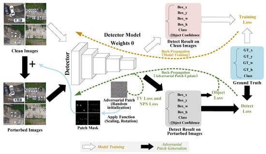
Figure 2.
The flowchart of the proposed method. The whole process consists of two parts: Part 1: Detection model training. This includes the optimization of the model’s weights. Part 2: Generating adversarial patch. First, the optimized adversarial patch is scaled, rotated, and attached to clean images, to generate perturbed images with the apply function. Second, the adversarial patch is continuously updated through the gradient ascent algorithm to minimize the loss function, which is the sum of four parts (object loss, detection loss, non-printability score (NPS) loss, and total variation (TV) loss).
Using the trained models, we consider generating adversarial patches on the two detectors. First, we initialize a random adversarial patch. Next, the clean images are transferred to the perturbed images by the apply function, which attaches the adversarial patch to all the objects. In this process, we should define the target ground truth for every object, and use it to construct the patch mask to determine where to attach the adversarial patch. Before the apply function, a series of transformations (patch rotation and rescale) are conducted on the adversarial patch to generate the patch mask. In particular, the rescaling of the patch depends on the scale factor. Then, to generate the perturbed images, we replace the pixel of the clean image with the pixel of the patch mask if the pixel of the patch mask is not zero. Finally, the perturbed images are input to the object detector to compute the loss function, consisting of object loss, detection loss, non-printability score (NPS) loss, and total variation (TV) loss. The adversarial patch is updated through the gradient ascent algorithm.
3.2. Problem Formulation
In this work, we focus on the digital attack and physical attack against two detectors, Yolo-V3 and Yolo-V5, which are widely used in object detection. Given an input image, and the target object detector . The outputs are a set of candidate bounding boxes , where . is the center of the box, and are the width and the height of the ith box, respectively, denotes the confidence if there is an object, and is the probability which decides the class of the box. The detectors may output a great number of bounding boxes in most cases, but most of them will be suppressed through non-maxima suppression (NMS) with a confidence threshold and intersecting over the union (IOU) threshold. This generally reminds us to minimize the confidence of the objects so that they can be filtered out to vanish under the object detector. An adversarial patch attack is considered in this work, and we add the adversarial patch to every object to hide all the objects under the two detectors. An adversarial patch is a frequently used method for physical attack, and is a kind of universal perturbation. In digital attack, the adversarial patch replaces some pixels of the objects to form an adversarial example. When it comes to the physical attack, the adversarial patch can be printed and placed on the objects. The adversarial example can be denoted as:
where denotes the adversarial example, P is the adversarial patch and denotes the apply function, which is aimed at attaching the adversarial patch to objects. Equation (1) shows the generation of the adversarial example of an adversarial patch attack. We attempt to generate a universal adversarial patch that may attack all car objects. The optimization process can be defined as:
where denotes non-maxima suppression, and is a count function which outputs the number of detected objects. and are the confidence threshold and IOU threshold, respectively. Equation (2) shows the target of the optimization. We hope that the detected objects are as few as possible after performing non-maxima suppression.
3.3. Transformations of Adversarial Patch
The perturbation of most attack methods can be classified as either global or local perturbation. However, most global perturbations are so small that they cannot work in the physical world in most cases. An adversarial patch is a kind of local and visible disturbance, which is expected to maintain its adversarial character in the physical world. It should be mentioned that the apply function is a vital tool when performing adversarial patch attacks, and it serves two functions. One is that we can attach the adversarial patch to the objects to generate the adversarial examples through the apply function. The other is that it can create a series of transformations (e.g., patch rotation and patch rescale) for the adversarial patch. Patch rotation makes the adversarial patch more robust in the physical world. Specifically, we generate a random rotation () on the embedded patch. To generate a universal adversarial patch that is valid for multi-scale objects, the adversarial patch needs to be scaled appropriately to adapt to the size of objects. To satisfy this requirement, we propose a method in which the patch size adapts to the height of the photography platform, which guarantees that the patch size is consistent in the same image. To be specific, by measuring the size of the objects in images captured at the height, we can compute the size to which the patch needs to be scaled. The scale factor can be calculated as shown in Equation (3).
where is the original size of the patch, is the size that the patch needs to be scaled for the images captured at the height of h and is the scale factor.
Finally, we can obtain a scale factor vector , where m denotes the number of flight heights. When performing a digital attack, the patch can be scaled to the corresponding size through Equation (3).
The size of the adversarial patch depends on the scale factor. Furthermore, in consideration of the feasibility in the real world, the patch needs to be placed in the proper location, such as the roof of the car, instead of the windows. Therefore, we should define the target ground truth for every object to determine where to attach the adversarial patch. Figure 3 shows that clean images are transferred to adversarial examples with the apply function. The size of the patch is matched to the size of the car roof, and the angle between the patch and the car is different after the random rotation of the patch.
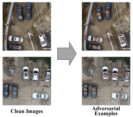
Figure 3.
Clean images and adversarial examples.
3.4. Adversarial Patch Optimization
To obtain a better attack effect, we propose a combination of detection loss and object loss to optimize adversarial patches. Furthermore, to make the physical attack more effective, we also introduce total variation (TV) loss and non-printability score (NPS) loss.
Object loss. As is analyzed in Section 3.2, object confidence denotes the probability of having an object. For an image, detection models usually output a large quantity of candidate bounding boxes, which are much more numerous than objects, which means there are several bounding boxes for one object. To filter out extra boxes, non-maximum suppression (NMS) is used in the detector. Firstly, it can suppress most of the candidate bounding boxes and retain those whose confidence is more than . The final results can be obtained by suppressing the bounding boxes whose value of IOU with the bounding box whose confidence is the largest, are more than . Hence, it is natural to take the confidence of the bounding box as the loss function.
The detection result depends on the bounding box whose confidence is more than . When attacking an object, the confidence of one bounding box is minimized so that it is less than the confidence threshold, but the other bounding boxes may work. Then, the object can still be detected. Furthermore, there may be many objects in a single remote-sensing image. Specifically, because of the open view in the air, it is often the case that a great number of objects are clustered in an image captured at a great height, which means the smaller the objects are, the greater the number of objects may be. The growth of the number of objects increases the level of threat and the difficulty of minimizing the confidence of all objects.
To ensure that more objects can be attacked, we propose taking the average object confidence as the object loss. The average object confidence is computed using all bounding boxes of all objects in one image, and object loss can be defined as:
In Equation (4), M denotes the number of bounding boxes of one image and refers to the confidence of the bounding box.
Detection loss. We concentrate on attacking Yolo-V3 and Yolo-V5 in this work. Before introducing detection loss, it is necessary to describe the loss of the training detection model. For model training, every object of the training set will be labeled so that they all have ground truths. If a bounding box is responsible for an object, will be set to 1. Then, the set of the ground truth can be described as , where , is the center of the ground truth box, and are the width and the height of the ith ground truth box, respectively, and decides the class of the ith box. Therefore, the loss as a result of optimizing the detection model consists of three parts, namely confidence loss, bounding box loss, and class loss. Confidence loss can be calculated with the binary cross-entropy , which can be calculated as shown in Equation (5).
where denotes the confidence if there is an object.
where is a hyperparameter that penalizes the incorrect objectness scores and denotes that the bounding box is responsible for an object. The first term in Equation (6) denotes the loss if there is an object in the bounding box, and the second term denotes the loss if there is no object in the bounding box.
Bounding box loss can be calculated with the squared error :
where is the center of the bounding box, and are the width and the height of the bounding box, is the center of the ground truth and and are the width and the height of the ground truth.
Class loss can be calculated with the binary cross-entropy :
where presents the probability which decides the class of the ground truth and denotes the probability which decides the class of the bounding box.
Equation (14) shows the train loss of a detector, which can be calculated by Equations (6), (11) and (13).
where , , and are the parameters to balance the weights of the three losses.
The detection model is trained by minimizing the loss. On the contrary, to attack the detection model, we consider maximizing the loss to degrade the accuracy of the model. Therefore, detection loss is as shown in Equation (15).
Total variation loss and non-printability score loss. In consideration of the adversarial effect in the physical world, we apply the total variation (TV) loss and the non-printability score (NPS) loss in this article, which are used to reduce distortion when the patch is applied in the physical world. TV loss is introduced to make the generated patch more smooth. Without the limitation of TV loss, the perturbation will be easily filtered out so that the attack performance decreases greatly. The TV loss is as shown in Equation (16).
where i and j denote the pixel coordinates of P.
The digital adversarial patch will be printed by the printer, which has a color space. If the pixel of the adversarial patch is not in the color space, there will be distortion between the digital domain and the physical domain for this pixel. Hence, the NPS loss is introduced to guarantee that the pixel color is in the color space of the printer, which reduces the distortion when the adversarial patch is printed. The NPS loss is as shown in Equation (17).
where P denotes adversarial patch, and is a digital pixel of P. C is the color space of the printer, and is an element of C.
The loss function is made up of four parts: object loss, detection loss, TV loss, and NPS loss. Object loss contributes to attacking more objects in one image. Detection loss is aimed at reducing the accuracy of the detection model. In this work, we propose the combination of detection loss and object loss, which is in favor of a better attack effect. The ablation experiment in Section 4.4 will verify the effectiveness of this method. The last two losses, TV loss and NPS loss, are used to reduce the distortion when the adversarial patch is applied in the physical world. The loss function can be calculated as shown in Equation (18).
where is a hyperparameter to balance the weight of .
4. Experiments
All of our experiments are designed on Yolo-V3 and Yolo-V5, and the remote sensing images we attacked were photographed by a UAV with heights ranging from 25 m to 120 m. First, the experimental setup is presented in Section 4.1. Then, the experimental results of digital attacks and the measurement of their effectiveness are presented in Section 4.2. Third, in Section 4.3, we report experiments that show the performance of our method in the physical world. Finally, several ablation studies are conducted to analyze the factors influencing the attack effect.
4.1. Experimental Setup
(1) Data collection. For the purpose of realizing adversarial attacks on multi-scale objects, some data containing multi-scale objects are needed. Naturally, we consider collecting data with a UAV at a vertical angle from different heights. To collect the data we require, we design a reasonable scheme for data capture. First, we choose two scenes as our experimental site, including a street and car park, where many kinds of cars are often seen. Afterward, we use DJI Mini 2 as the capturing tool. In our scheme, the flight height ranges from 25 m to 120 m with a height interval of 5 m, so there were 20 flight heights in total. The resolution of the raw images is 3840 × 2160. However, this size is too large, being unsuitable for our experiment. Therefore, we need to conduct some processing of the raw images. They are first tailored into a smaller size of 960 × 960, and then are resized to 640 × 640 when being attacked. Ultimately, there are 253 training images with 1680 car objects and 186 testing images with 748 car objects. For physical attacks, the generated adversarial patches in the digital domain are printed and put on the proof of the cars. In the same way, the images in physical experiments are captured at different heights. Figure 4 shows several images captured by a UAV from the heights of 30 m, 60 m and 120 m, respectively. The size of the objects is quite diverse, and the number of objects in a single image is large, especially for images captured at a great height.
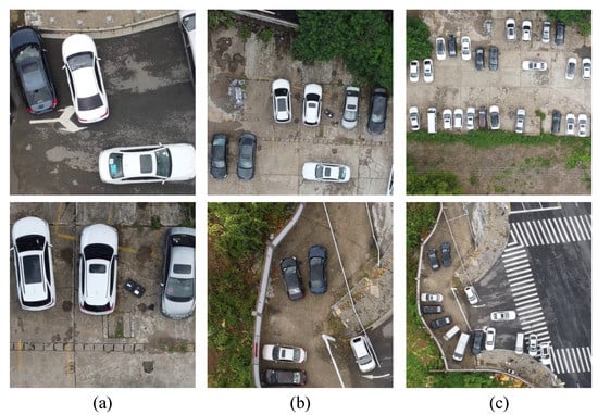
Figure 4.
(a) Images captured at the height of 30 m. (b) Images captured at the height of 60 m. (c) Images captured at the height of 120 m. The variation in photography height causes the objects to vary greatly in size.
(2) Detectors. Yolo models are typical object detectors. With their continuous improvement and renewal, several versions of Yolo have arisen, such as Yolo-V3 [10], Yolo-V4 [11], Yolo-V5 [12], Yolo-V6 [13] and Yolo-V7 [14]. They have attained better performance and higher speed for real-time reasoning. Yolo-V3 and Yolo-V5 in particular are popular algorithms that are widely used in object detection. Therefore, we choose Yolo-V3 and Yolo-V5 based on ultralytics as our target models. As for model training, we select the visdrone2019 dataset as our training dataset for two reasons: one is that it is a remote sensing dataset of UAV, and the other is its higher resolution. To satisfy the requirements of our experiments, we conduct some adjustments to the dataset. Only the car objects are retained in the labels, and the others are removed. Then, we delete those images that do not contain a car object. Ultimately, there are 6132 training images and 515 testing images left for model training. The input size of the two models is fixed at 640 × 640 when training.
(3) Baseline methods. To evaluate the effectiveness of our method, several experiments are designed to compare our method with other methods, including OBJ [33], Dpatch [46] and Patch-Noobj [42], which are all patch attack methods.
(4) Metrics and implementation details. Currently, most methods regard the average precision (AP) as the evaluation metric. However, we feel that this is not a proper criterion, because a high number of false alarms may also degrade the value of AP, but the true objects can still be detected when the false alarm rate increases. To develop a better evaluation, we adopt the attack success rate (ASR) metrics as our evaluation metrics. The ASR can be expressed as follows:
where denotes the sum of objects whose confidence is less than the threshold . denotes the sum of all objects in the test data. We define the object as being attacked successfully if there is no detection box on the object. Six confidence thresholds ( = 0.1, 0.2, 0.3, 0.4, 0.5, 0.6) are selected to show the effectiveness of our method.
For digital attack evaluation, the test data are divided into 5 groups based on the height of photography (Group 1: 25–40 m, Group 2: 45–60 m, Group 3: 65–80 m, Group 4: 85–100 m, and Group 5: 105–120 m) and the ASR is evaluated for all 5 groups. Furthermore, we use the same approach to evaluate the physical attack effect.
In terms of implementation details, we set the batch size as 3, and the maximum number of epochs as 200. All the experiments are realized in PyTorch, and our desktop is equipped with an Intel Core i9-10900X CPU and an Nvidia RTX-3090 GPU. For the sake of fairness, all experiments are carried out in the same conditions.
4.2. Digital Attack
In this section, we perform digital experiments to test the ASR using our method, OBJ [33], DPatch [46], and Patch-Noobj [42] on Yolo-V3 and Yolo-V5. For the sake of fairness, all experiments for the four methods are carried out in the same conditions. For example, in Dpatch, there is originally one adversarial patch for one image, but we place the adversarial patch on every object in our experiments, which guarantees that the conditions are the same as for the other three methods. To prove that our method has a better attack effect for different-scale objects, we divide the test data into 5 groups. In particular, we evaluate the ASR for different scales and compute the total ASR for all test data. Finally, a comprehensive analysis of the evaluation results was conducted.
The experimental results for Yolo-V3 are shown in Table 1. First, the attack effect of every group is evaluated. It is obvious that our method outperforms the other methods in most cases. We can see from the data of Table 1 that Patch-Noobj and DPatch show better performance for small-scale objects than large-scale objects. Moreover, OBJ performs better for large-scale objects than small-scale objects. Specifically, our method shows good performance for all groups. Taking a confidence level of 0.5 as an example, the ASRs of Patch-Noobj and DPatch are 40.00% and 46.62% and 2.00% and 1.35% for the first two groups, which are much less than 96.00% and 93.92% for our method. The overall attack effect of OBJ is better than DPatch and Patch-Noobj, but is still inferior to our method in the majority of the cases.

Table 1.
Experimental results of different scales (25–120 m) and different confidence levels (0.1–0.6) for Yolo-V3. Specifically, the bold and underlined values indicate the sota and the second best.
When we focus on the different confidence levels, it can be seen that our method is superior for all. The ASR of our method with a confidence of 0.1 for all groups is more than 70% for Yolo-V3. As confidence increases, our method stays on top in most cases. The ASR of our method is ranked first among all groups in all confidence levels, except Group 1 with a confidence of 0.5 and 0.6. The total ASRs of our method are 80.61%, 85.56%, 88.50%, 90.51%, 92.65%, and 94.53% for six different confidence thresholds, which are all the best of the four methods, being head and shoulders above the second best.
Table 2 shows the attack results for Yolo-V5. It can be found that the attack performance for Yolo-V5 is not as good as Yolo-V3 for all four methods. That may be because the architecture of Yolo-V5 is more robust than Yolo-V3. Nevertheless, our method has a significant advantage compared with the other methods in terms of the ASR of different groups and the total ASR under different confidences. It can be seen that DPatch and Patch-Noobj have little effect on large-scale objects. The overall attack effect of OBJ is better than that of DPatch and Patch-Noobj, but poorer than our method.
Table 2.
Experimental results of different scales (25–120 m) and different confidence levels (0.1–0.6) for Yolo-V5. Specifically, the bold and underlined values indicate the best and the second best.
Similar to the attack effect of Yolo-V3, as confidence increases, the ASRs of every method increase, and our method stays on top in most cases. The total ASRs of our method are 18.05%, 31.02%, 40.37%, 51.20%, 60.16%, and 69.52% for six different confidence thresholds, which are all the best of the four methods, being head and shoulders above the second best.
The conclusion can be drawn from Table 1 and Table 2 that the performance of our method is the best in the majority of cases and is the second best in other cases, which demonstrates the superiority of our method for multi-scale object attack. These results may be due to the optimization of the proposed method. contributes to attacking as many objects as possible, because the computation of refers to all objects. , which aims at degrading the accuracy of the detection model, also has a positive effect in attacking the detector, and the ablation studies in Section 4.4 verify this point.
Furthermore, we provide visualizations of the adversarial patch and attack results for different methods in Figure 5 and Figure 6. Figure 5 shows the attack results for Yolo-V3 and Figure 6 shows the attack results for Yolo-V5. For Yolo-V3, images captured from 30 m, 90 m, and 120 m are selected, and for Yolo-V5, images captured from 40 m, 80 m, and 120 m are selected to show the attack effect. It can be observed that our adversarial patch attack affects more objects than the other three methods. DPatch and Patch-Noobj show better performance in small objects than in large objects. Observing the texture of the adversarial patch, we may find that the patch texture of DPatch and Patch-Noobj seems to be representative of cars. Therefore, if the size of the patch is large, the texture will be easily detected as cars, which leads to the object being unable to vanish thoroughly. One intuitive reason for this phenomenon is that DPatch takes the of the detector as the target loss and Patch-Noobj takes as the target loss. These two losses both aim at degrading the accuracy of the detector. However, low accuracy is not equal to high ASR, because false alarms also lead to bad accuracy, but the object may not disappear thoroughly. For our method, there is no texture suggestive of a car in the adversarial patch, and owing to the combination of detection loss and object loss in our loss function, the attack effect is better than that of DPatch, Patch-Noobj, and OBJ. Furthermore, we may find that the textures between Yolo-V3 and Yolo-V5 are different, which proves that texture also depends on the architecture of the detection model. In spite of this, similar conclusions can be drawn about the attack effect for Yolo-V3 and Yolo-V5.
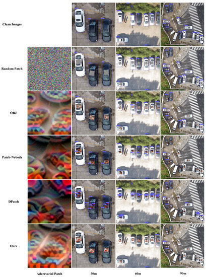
Figure 5.
Comparison of the attack effects for our method, Dpatch, OBJ, Patch-Noobj and random patch for Yolo-V3. Images shown in this figure were captured at heights of 30 m, 60 m and 90 m.
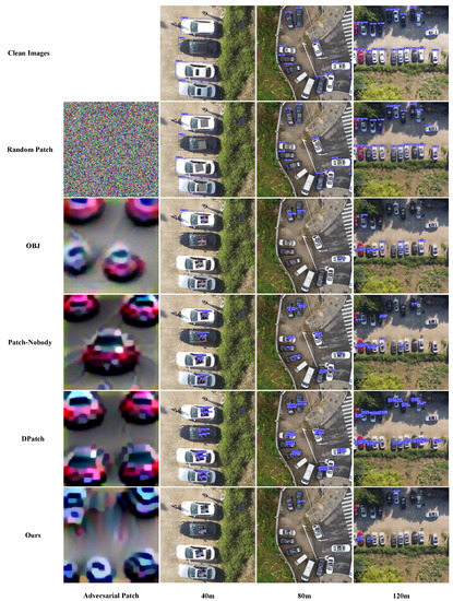
Figure 6.
Comparison of the attack effects for our method, Dpatch, OBJ, Patch-Noobj and random patch for Yolo-V5. Images shown in this figure were captured at heights of 30 m, 60 m and 90 m.
4.3. Physical Attack
The physical attack results of our method on Yolo-V3 and Yolo-V5 will be shown in this section. In view of the actual size of the car, the generated adversarial patches are printed with a size of 1.1 m × 1.1 m. When carrying out the physical attack, the adversarial patches are placed on the roofs of cars. We use the DJI Mini2 to capture videos that contain cars covered with adversarial patches from 20 m to 120 m. Similar to the strategy used for digital attack, we divide these data into five groups (Group 1: 20–40 m, Group 2: 40–60 m, Group 3: 60–80 m, Group 4: 80–100 m, and Group 5: 100–120 m).
We further preprocess the captured data. Firstly, the videos should be cut according to the flight height. Then, the videos that have been cut are sent to the detection model to output the detection result. To better evaluate the physical attack effect, we process the videos that have been detected as frame-by-frame images. For physical attacks, we take ASR as the evaluation metric and the confidence threshold is set to 0.5. In our experiments, only the objects covered with adversarial patches are valid for computing the ASR. Table 3 shows the number of objects in every group for Yolo-V3 and Yolo-V5.
Table 3.
The numbers of objects with adversarial patch for Yolo-V3 and Yolo-V5.
The physical attack results are shown in Table 4. It can be observed that the ASRs of Group 1, Group 2, and Group 3 are much higher than those of Group 4 and Group 5 for Yolo-V3 and Yolo-V5. These results may be attributed to image degradation. In real scenarios, low-resolution images suffer from some degradation, which usually arises from complicated combinations of degradation processes, such as the imaging systems of cameras, image editing, and Internet transmission. Therefore, when we capture an image, there will be some distortion in this image, and the object in this image will appear to be different from the real object. Similarly, when carrying out the experiments of physical attack, as the resolution of the adversarial patch decreases, the adversarial patch also suffers from the degradation of the real world, which leads to poor performance for physical attack.
Table 4.
Physical attack results on Yolo-V3 and Yolo-V5.
Some selected examples of physical attacks on Yolo-V3 and Yolo-V5 are presented in Figure 7 and Figure 8. Figure 7 shows several images of three scenes for Yolo-V3 and Figure 8 shows several images of three scenes for Yolo-V5. It can be observed that the attack results for Group 1, Group 2, and Group 3 are better than those for Group 4 and Group 5. Moreover, we find that the adversarial patches suffer from serious degradation as the size of the object decreases, which is the reason for the poor attack results.
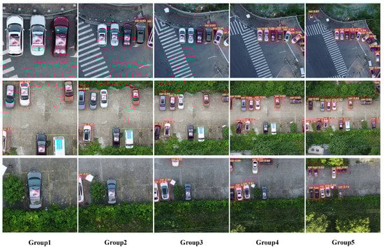
Figure 7.
Selected examples of physical attacks on Yolo-V3. These examples are from three scenes, and the images in the same row are from the same scene. For every scene, we select five images from five groups.
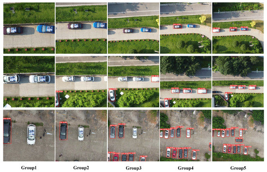
Figure 8.
Selected examples of physical attacks on Yolo-V5. These examples are from three scenes, and the images in the same row are from the same scene. For every scene, we select five images from five groups.
4.4. Ablation Studies
To evaluate how each loss of the proposed method influences the attack performance, quantitative ablation studies are carried out.
Table 5 and Table 6 show the attack results with different combinations of detection loss and object loss for Yolo-V3 and Yolo-V5. Comparing the results of object loss in Table 5 and Table 6 with the results of other methods in Table 1 and Table 2, we can find that the success rates of object loss in Group 3, Group 4 and Group 5 (the size of objects in these groups is smaller and the number of objects in a single image is larger) are all the best for two detectors, which verifies that contributes to attacking as many objects as possible. Furthermore, directly using detection loss alone only leads to poor performance, while combining detection loss and object loss can obtain a better attack effect. From the perspective of the experimental results, we may find that object loss plays a major role in ASR. However, with the help of detection loss, higher ASR may be gained for different scales. Moreover, we explore the influence of different values of for detection loss. It is found that the best is 0.02 for Yolo-V3 and the best is 0.005 for Yolo-V5.
Table 5.
Experimental results of different loss items for Yolo-V3. Bold fonts indicate the best effect.
Table 6.
Experimental results of different loss items for Yolo-V5. Bold fonts indicate the best effect.
Table 7 shows the attack effect on AP, precision, and recall, which are evaluation metrics for the detection model. It can be observed that the performance of the proposed methods is not the best and detection loss has the lowest score for the three parameters, whether for Yolo-V3 or Yolo-V5, which proves that detection loss plays an important role in decreasing the accuracy of the model. One intuitive reason for this result is that the proposed loss may sacrifice a little of the attack performance of AP, precision, and recall to achieve attacking more objects. It can be concluded that the object loss may work better with the degradation of the model’s accuracy.
Table 7.
Comparison of attack effect on AP, precision, and recall. Bold fonts indicate the best effect.
5. Conclusions
In this study, we evaluate the attack effect on objects of different scales in UAV remote sensing data for the first time, and we perform a physical adversarial attack on multi-scale objects. First, we formulate a joint optimization problem, in which object loss and detection loss are introduced, to generate a universal adversarial patch. Object loss, which denotes the average confidence of all bounding boxes in one image, contributes to attacking as many objects as possible. Detection loss between the detection results and the ground truth aims to degrade the accuracy of a detector. The experimental results demonstrate the effectiveness of the combination of the two losses. Furthermore, we raise a scale factor to allow the scale of the adversarial patch to adapt to the size of the object for the digital attack, which ensures that the adversarial patch is valid for multi-scale objects in the real world. Images for adversarial attacks are captured from 25 m to 120 m using DJI Mini 2. In our experiments, we divide the test data into five groups based on the height label of the images. Several digital attack experiments for Yolo-V3 and Yolo-V5 are carried out, and we compute the ASR for six confidences (0.1, 0.2, 0.3, 0.4, 0.5, and 0.6). For ASR of different scales, our method outperforms state-of-the-art methods in most cases. For the total ASR, our method also outperforms other methods for every confidence level. Furthermore, the generated adversarial patch of our method is printed, and we perform physical attack experiments to verify the attack effect for different photography heights.
Although our method has a great effect on the digital attack, the attack effect is diminished when it is used in the real world. For future works, we will consider several research directions to solve the problem of the physical attack effect not being satisfactory when the photography height changes. First, the coverage areas of objects are limited, which results in non-ideal effects. We will therefore aim to cover more areas to enhance the attack effect. Second, we will try to solve the problem of the attack effect fading as a result of real-world degradation.
Author Contributions
Conceptualization, Y.Z. (Yichuang Zhang); methodology, Y.Z (Yichuang Zhang). and P.Z.; software, Y.Z. (Yichuang Zhang); validation, Y.Z. (Yichuang Zhang); formal analysis, Y.Z. (Yichuang Zhang).; investigation, Y.Z. (Yichuang Zhang); resources, P.Z.; writing—original draft preparation, Y.Z. (Yichuang Zhang); writing—review and editing, Y.Z. (Yichuang Zhang), Y.Z. (Yu Zhang), J.Q., K.B., H.W., X.T. and P.Z.; visualization, Y.Z. (Yichuang Zhang); supervision, P.Z.; project administration, P.Z. All authors have read and agreed to the published version of the manuscript.
Funding
This work was supported in part by the Natural Science Foundation of China under Grant 61971428.
Data Availability Statement
Data sharing is not applicable to this article.
Conflicts of Interest
The authors declare no conflict of interest.
References
- Liu, R.; Kuffer, M.; Persello, C. The Temporal Dynamics of Slums Employing a CNN-Based Change Detection Approach. Remote Sens. 2019, 11, 2844. [Google Scholar] [CrossRef]
- Peng, B.; Meng, Z.; Huang, Q.; Wang, C. Patch Similarity Convolutional Neural Network for Urban Flood Extent Mapping Using Bi-Temporal Satellite Multispectral Imagery. Remote Sens. 2019, 11, 2492. [Google Scholar] [CrossRef]
- Zhang, X.; Han, L.; Dong, Y.; Shi, Y.; Huang, W.; Han, L.; González-Moreno, P.; Ma, H.; Ye, H.; Sobeih, T. A Deep Learning-Based Approach for Automated Yellow Rust Disease Detection from High-Resolution Hyperspectral UAV Images. Remote Sens. 2019, 11, 1554. [Google Scholar] [CrossRef]
- Liu, H.; Li, J.; He, L.; Wang, Y. Superpixel-Guided Layer-Wise Embedding CNN for Remote Sensing Image Classification. Remote Sens. 2019, 11, 174. [Google Scholar] [CrossRef]
- Matos-Carvalho, J.P.; Moutinho, F.; Salvado, A.B.; Carrasqueira, T.; Campos-Rebelo, R.; Pedro, D.; Campos, L.M.; Fonseca, J.M.; Mora, A. Static and Dynamic Algorithms for Terrain Classification in UAV Aerial Imagery. Remote Sens. 2019, 11, 2501. [Google Scholar] [CrossRef]
- Guan, Z.; Miao, X.; Mu, Y.; Sun, Q.; Ye, Q.; Gao, D. Forest Fire Segmentation from Aerial Imagery Data Using an Improved Instance Segmentation Model. Remote Sens. 2022, 14, 3159. [Google Scholar] [CrossRef]
- Ren, S.; He, K.; Girshick, R.; Sun, J. Faster R-CNN: Towards Real-Time Object Detection with Region Proposal Networks. Adv. Neural Inf. Process. Syst. 2015, 28, 91–99. [Google Scholar] [CrossRef]
- Liu, W.; Anguelov, D.; Erhan, D.; Szegedy, C.; Reed, S.; Fu, C.Y.; Berg, A.C. SSD: Single Shot Multibox Detector. In Proceedings of the European Conference on Computer Vision (ECCV), Amsterdam, The Netherlands, 8–16 October 2016; pp. 21–37. [Google Scholar]
- Redmon, J.; Divvala, S.; Girshick, R.; Farhadi, A. You Only Look Once: Unified, Real-Time Object Detection. In Proceedings of the 2015 IEEE Conference on Computer Vision and Pattern Recognition (CVPR), Boston, MA, USA, 7–12 June 2015; pp. 779–788. [Google Scholar]
- Redmon, J.; Farhadi, A. Yolov3: An Incremental Improvement. arXiv 2018, arXiv:1804.02767. [Google Scholar]
- Bochkovskiy, A.; Wang, C.Y.; Liao, H.Y.M. Yolov4: Optimal Speed and Accuracy of Object Detection. arXiv 2020, arXiv:2004.10934. [Google Scholar]
- Jocher, G.; Stoken, A.; Borovec, J.; Tao, X.; Kwon, Y.; Michael, K.; Liu, C.; Fang, J.; Abhiram, V.; Skalski, P.; et al. Ultralytics/yolov5: V6.0—YOLOv5n ‘Nano’ Models, Roboflow Integration, TensorFlow Export, OpenCV DNN Support. Available online: https://zenodo.org/record/5563715#.Y0Y3nmdBy3B (accessed on 20 September 2021).
- Li, C.; Li, L.; Jiang, H.; Weng, K.; Geng, Y.; Li, L.; Ke, Z.; Li, Q.; Cheng, M.; Nie, W.; et al. YOLOv6: A Single-Stage Object Detection Framework for Industrial Applications. arXiv 2022, arXiv:2209.02976. [Google Scholar]
- Wang, C.Y.; Bochkovskiy, A.; Liao, H.Y.M. YOLOv7: Trainable Bag-of-Freebies Sets New State-of-the-Art for Real-Time Object Detectors. arXiv 2022, arXiv:2207.02696. [Google Scholar]
- Dong, X.; Qin, Y.; Gao, Y.; Fu, R.; Liu, S.; Ye, Y. Attention-Based Multi-Level Feature Fusion for Object Detection in Remote Sensing Images. Remote Sens. 2022, 14, 3735. [Google Scholar] [CrossRef]
- Zhao, Y.; Li, J.; Li, W.; Shan, P.; Wang, X.; Li, L.; Fu, Q. MS-IAF: Multi-Scale Information Augmentation Framework for Aircraft Detection. Remote Sens. 2022, 14, 3696. [Google Scholar] [CrossRef]
- Zheng, Y.; Sun, P.; Zhou, Z.; Xu, W.; Ren, Q. ADT-Det: Adaptive Dynamic Refined Single-Stage Transformer Detector for Arbitrary-Oriented Object Detection in Satellite Optical Imagery. Remote Sens. 2021, 13, 2623. [Google Scholar] [CrossRef]
- Mohamed, A.R.; Dahl, G.E.; Hinton, G. Acoustic Modeling Using Deep Belief Networks. IEEE Trans. Audio Speech Lang. Process. 2011, 20, 14–22. [Google Scholar] [CrossRef]
- Sutskever, I.; Vinyals, O.; Le, Q.V. Sequence to Sequence Learning with Neural Networks. In Proceedings of the 27th International Conference on Neural Information Processing Systems (NeurIPS), Montreal, QC, Canada, 8–13 December 2014; pp. 3104–3112. [Google Scholar]
- Krizhevsky, A.; Sutskever, I.; Hinton, G.E. Imagenet Classification With Deep Convolutional Neural Networks. In Proceedings of the 26th Annual Conference on Neural Information Processing Systems (NeurIPS), Lake Tahoe, NV, USA, 3–6 December 2012; pp. 1097–1105. [Google Scholar]
- Qin, H.; Cai, Z.; Zhang, M.; Ding, Y.; Zhao, H.; Yi, S.; Liu, X.; Su, H. Bipointnet: Binary Neural Network for Point Clouds. arXiv 2020, arXiv:2010.05501. [Google Scholar]
- Szegedy, C.; Zaremba, W.; Sutskever, I.; Bruna, J.; Erhan, D.; Goodfellow, I.; Fergus, R. Intriguing Properties of Neural Networks. arXiv 2013, arXiv:1312.6199. [Google Scholar]
- Goodfellow, I.J.; Shlens, J.; Szegedy, C. Explaining and Harnessing Adversarial Examples. arXiv 2014, arXiv:1412.6572. [Google Scholar]
- Madry, A.; Makelov, A.; Schmidt, L.; Tsipras, D.; Vladu, A. Towards Deep Learning Models Resistant to Adversarial Attacks. arXiv 2017, arXiv:1706.06083. [Google Scholar]
- Moosavi-Dezfooli, S.M.; Fawzi, A.; Frossard, P. DeepFool: A Simple and Accurate Method to Fool Deep Neural Networks. In Proceedings of the 2016 IEEE Conference on Computer Vision and Pattern Recognition (CVPR), Las Vegas, NV, USA, 27–30 June 2016; pp. 2574–2582. [Google Scholar]
- Moosavi-Dezfooli, S.M.; Fawzi, A.; Fawzi, O.; Frossard, P. Universal Adversarial Perturbations. In Proceedings of the IEEE Conference on Computer Vision and Pattern Recognition (CVPR), Honolulu, HI, USA, 21–26 July 2017; pp. 1765–1773. [Google Scholar]
- Carlini, N.; Wagner, D. Towards Evaluating the Robustness of Neural Networks. In Proceedings of the 2017 IEEE Symposium on Security and Privacy (SP), San Jose, CA, USA, 22–26 May 2017; pp. 39–57. [Google Scholar]
- Papernot, N.; McDaniel, P.; Jha, S.; Fredrikson, M.; Celik, Z.B.; Swami, A. The Limitations of Deep Learning in Adversarial Settings. In Proceedings of the 2016 IEEE European Symposium on Security and Privacy (EuroS&P), Saarbrücken, Germany, 21–24 March 2016; pp. 372–387. [Google Scholar]
- Sharif, M.; Bhagavatula, S.; Bauer, L.; Reiter, M.K. Accessorize to a Crime: Real and Stealthy Attacks on State-of-the-art Face Recognition. In Proceedings of the 2016 ACM Sigsac Conference on Computer Furthermore, Communications Security (CCS), Vienna, Austria, 24–28 October 2016; pp. 1528–1540. [Google Scholar]
- Xu, K.; Zhang, G.; Liu, S.; Fan, Q.; Sun, M.; Chen, H.; Chen, P.Y.; Wang, Y.; Lin, X. Adversarial T-Shirt! Evading Person Detectors in a Physical World. In Proceedings of the European Conference on Computer Vision (ECCV), Glasgow, UK, 23–28 August 2020; pp. 665–681. [Google Scholar]
- Brown, T.B.; Mané, D.; Roy, A.; Abadi, M.; Gilmer, J. Adversarial Patch. arXiv 2017, arXiv:1712.09665. [Google Scholar]
- Kurakin, A.; Goodfellow, I.J.; Bengio, S. Adversarial examples in the Physical World. In Proceedings of the Workshop of the 5th International Conference on Learning Representations (ICLR), Toulon, France, 24–26 April 2017. [Google Scholar]
- Thys, S.; Van Ranst, W.; Goedemé, T. Fooling Automated Surveillance Cameras: Adversarial Patches to Attack Person Detection. In Proceedings of the IEEE/CVF Conference on Computer Vision and Pattern Recognition Workshops (CVPRW), Long Beach, CA, USA, 16–17 June 2019. [Google Scholar]
- Hu, Z.; Huang, S.; Zhu, X.; Sun, F.; Zhang, B.; Hu, X. Adversarial Texture for Fooling Person Detectors in the Physical World. In Proceedings of the IEEE/CVF Conference on Computer Vision and Pattern Recognition (CVPR), New Orleans, LA, USA, 19–24 June 2022; pp. 13307–13316. [Google Scholar]
- Xu, Y.; Du, B.; Zhang, L. Assessing the Threat of Adversarial Examples on Deep Neural Networks for Remote Sensing Scene Classification: Attacks and Defenses. IEEE Trans. Geosci. Remote Sens. 2020, 59, 1604–1617. [Google Scholar] [CrossRef]
- Chan-Hon-Tong, A.; Lenczner, G.; Plyer, A. Demotivate Adversarial Defense in Remote Sensing. In Proceedings of the 2021 IEEE International Geoscience and Remote Sensing Symposium (IGARSS), Brussels, Belgium, 11–16 July 2021; pp. 3448–3451. [Google Scholar]
- Chen, L.; Zhu, G.; Li, Q.; Li, H. Adversarial Example in Remote Sensing Image Recognition. arXiv 2019, arXiv:1910.13222. [Google Scholar]
- Czaja, W.; Fendley, N.; Pekala, M.; Ratto, C.; Wang, I.J. Adversarial Examples in Remote Sensing. In Proceedings of the 26th ACM SIGSPATIAL International Conference on Advances in Geographic Information Systems (ACM SIGSPATIAL 2018), Seattle, WA, USA, 6–9 November 2018; pp. 408–411. [Google Scholar]
- Xu, Y.; Ghamisi, P. Universal Adversarial Examples in Remote Sensing: Methodology and Benchmark. IEEE Trans. Geosci. Remote Sens. 2022, 60, 1–15. [Google Scholar] [CrossRef]
- Chen, L.; Xu, Z.; Li, Q.; Peng, J.; Wang, S.; Li, H. An Empirical Study of Adversarial Examples on Remote Sensing Image Scene Classification. IEEE Trans. Geosci. Remote Sens. 2021, 59, 7419–7433. [Google Scholar] [CrossRef]
- Xu, Y.; Du, B.; Zhang, L. Self-Attention Context Network: Addressing the Threat of Adversarial Attacks for Hyperspectral Image Classification. IEEE Trans. Image Process. 2021, 30, 8671–8685. [Google Scholar] [CrossRef] [PubMed]
- Lu, M.; Li, Q.; Chen, L.; Li, H. Scale-Adaptive Adversarial Patch Attack for Remote Sensing Image Aircraft Detection. Remote Sens. 2021, 13, 4078. [Google Scholar] [CrossRef]
- Du, A.; Chen, B.; Chin, T.J.; Law, Y.W.; Sasdelli, M.; Rajasegaran, R.; Campbell, D. Physical Adversarial Attacks on an Aerial Imagery Object Detector. In Proceedings of the Proceedings of the IEEE/CVF Winter Conference on Applications of Computer Vision (WACV), Waikoloa, HI, USA, 4–8 January 2022; pp. 1796–1806. [Google Scholar]
- den Hollander, R.; Adhikari, A.; Tolios, I.; van Bekkum, M.; Bal, A.; Hendriks, S.; Kruithof, M.; Gross, D.; Jansen, N.; Perez, G.; et al. Adversarial patch camouflage against aerial detection. In Proceedings of the Artificial Intelligence and Machine Learning in Defense Applications II, Online, 21–25 September 2020; Volume 11543, p. 115430F. [Google Scholar]
- Chow, K.H.; Liu, L.; Gursoy, M.E.; Truex, S.; Wei, W.; Wu, Y. TOG: Targeted Adversarial Objectness Gradient Attacks on Real-Time Object Detection Systems. arXiv 2020, arXiv:2004.04320. [Google Scholar]
- Liu, X.; Yang, H.; Liu, Z.; Song, L.; Li, H.; Chen, Y. Dpatch: An Adversarial Patch Attack on Object Detectors. arXiv 2018, arXiv:1806.02299. [Google Scholar]
- Athalye, A.; Engstrom, L.; Ilyas, A.; Kwok, K. Synthesizing Robust Adversarial Examples. In Proceedings of the International Conference on Machine Learning (ICML), Stockholm, Sweden, 10–15 July 2018; pp. 284–293. [Google Scholar]
- Evtimov, I.; Eykholt, K.; Fernandes, E.; Kohno, T.; Li, B.; Prakash, A.; Rahmati, A.; Song, D. Robust Physical-World Attacks on Deep Learning Models. In Proceedings of the 2018 IEEE/CVF Conference on Computer Vision and Pattern Recognition (CVPR), Salt Lake City, UT, USA, 18–23 June 2018. [Google Scholar]
- Chen, S.T.; Cornelius, C.; Martin, J.; Chau, D.H.P. Shapeshifter: Robust Physical Adversarial Attack on Faster R-CNN Object Detector. In Proceedings of the Joint European Conference on Machine Learning and Knowledge Discovery in Databases (ECML-PKDD), Dublin, Ireland, 10–14 September 2018; pp. 52–68. [Google Scholar]
- Eykholt, K.; Evtimov, I.; Fernandes, E.; Li, B.; Song, D.; Kohno, T.; Rahmati, A.; Prakash, A.; Tramer, F. Note on Attacking Object Detectors with Adversarial Stickers. arXiv 2017, arXiv:1712.08062. [Google Scholar]
- Lu, J.; Sibai, H.; Fabry, E. Adversarial Examples That Fool Detectors. arXiv 2017, arXiv:1712.02494. [Google Scholar]
- Song, D.; Eykholt, K.; Evtimov, I.; Fernandes, E.; Li, B.; Rahmati, A.; Tramer, F.; Prakash, A.; Kohno, T. Physical Adversarial Examples for Object Detectors. In Proceedings of the 12th USENIX Workshop on Offensive Technologies (WOOT 2018), Co-Located with USENIX Security 2018, Baltimore, MD, USA, 13–14 August 2018. [Google Scholar]
- Redmon, J.; Farhadi, A. YOLO9000: Better, Faster, Stronger. In Proceedings of the 30th IEEE Conference on Computer Vision and Pattern Recognition (CVPR), Honolulu, HI, USA, 21–26 July 2017; pp. 6517–6525. [Google Scholar]
- Wang, Y.; Lv, H.; Kuang, X.; Zhao, G.; Tan, Y.A.; Zhang, Q.; Hu, J. Towards a Physical-World Adversarial Patch for Blinding Object Detection Models. Inf. Sci. 2021, 556, 459–471. [Google Scholar] [CrossRef]
- Wang, J.; Liu, A.; Yin, Z.; Liu, S.; Tang, S.; Liu, X. Dual Attention Suppression Attack: Generate Adversarial Camouflage in Physical World. In Proceedings of the IEEE/CVF Conference on Computer Vision and Pattern Recognition (CVPR), Nashville, TN, USA, 20–25 June 2021; pp. 8565–8574. [Google Scholar]


Publisher’s Note: MDPI stays neutral with regard to jurisdictional claims in published maps and institutional affiliations. |
© 2022 by the authors. Licensee MDPI, Basel, Switzerland. This article is an open access article distributed under the terms and conditions of the Creative Commons Attribution (CC BY) license (https://creativecommons.org/licenses/by/4.0/).