Article

Estimating Soil Organic Matter Content in Desert Areas Using In Situ Hyperspectral Data and Feature Variable Selection Algorithms in Southern Xinjiang, China

1
College of Agriculture, Tarim University, Alar 843300, China
2
Department of Soil Science, University of Wisconsin-Madison, Madison, WI 53706, USA
3
Department of Land Resource Management, School of Tourism and Urban Management, Jiangxi University of Finance and Economics, Nanchang 330013, China
*
Author to whom correspondence should be addressed.
Remote Sens. 2022, 14(20), 5221; https://doi.org/10.3390/rs14205221
Submission received: 14 August 2022 / Revised: 1 October 2022 / Accepted: 15 October 2022 / Published: 18 October 2022
(This article belongs to the Special Issue Topsoil Characterization by Means of Remote Sensing)

Abstract

:
Soil organic matter (SOM) is a key factor for evaluating soil fertility. Rapidly monitoring organic matter content in desert soil can provide a scientific basis for the rational development and utilization of reserve arable land resources. Although spectral inversion accuracy for SOM under laboratory-controlled conditions is high, it is time-consuming and costly compared to the in situ spectroscopic determination method. However, in situ spectroscopy causes losses in accuracy due to interference from external environmental factors (e.g., the surface roughness of soil, changes in weather conditions, atmospheric water vapor, etc.). Therefore, reducing or removing the interference of external environmental factors to improve the accuracy of in situ spectroscopy for estimating SOM is challenging. In this study, visible and near-infrared (Vis-NIR) in situ spectral data were collected from 135 topsoil (0–20 cm) samples in a desert area of northwestern China, and organic matter content was measured. Three spectral pre-processing methods—the standard normal transform (SNV), reciprocal logarithm (log(1/R)) and normalization (NOR)—combined with three feature variable selection methods—the particle swarm algorithm (PSO), ant colony algorithm (ACO) and simulated annealing (SA) algorithm—were used to filter the spectral feature bands of SOM, and then partial least squares regression (PLSR), a back propagation neural network (BPNN) and a convolutional neural network (CNN) were used to construct the estimation models of SOM. The results indicated that the SNV could enhance the spectral information related to SOM and improve the accuracy of model estimation, and it was one of the most effective spectral pretreatment methods. Compared with the model constructed with the full-band spectroscopy method, the feature variable selection method could effectively improve the estimation accuracy of the Vis-NIR in situ spectroscopy model. The most obvious improvement was found with PSO, where R2 and RPD were improved by more than 0.34 and 0.16, respectively, and RMSE was reduced by more than 0.29 g kg−1. The accuracy of the CNN model was higher than that of the BPNN and PLSR models, both for the inversion model of SOM built from full-band spectral data and the bands selected by the characteristic variable selection method. SNV-PSO-CNN is the optimal hybrid model for in situ spectral measurement of SOM (R2 = 0.71, RPD = 1.88, RMSE = 1.67 g kg−1) and can realize the quantitative in situ spectral inversion of SOM in desert soils.

1. Introduction

Soil organic matter (SOM) is both a dominant source of nutrients for crops and an important indicator of soil fertility. Soil organic carbon (SOC) is a major component of SOM, making up about 58% of its mass [1]. The rapid monitoring of SOM content and dynamics provides a scientific basis for the reclamation of arable land and environmental protection [2,3,4]. The traditional approach for SOM determination requires the collection of soil samples and laboratory analyses and measurements, which limit the efficiency of SOM monitoring due to the large demands in cost and time. Hyperspectral technology, a relatively new approach for SOM prediction, can overcome the limitations of traditional laboratory measurements and quickly obtain information on a variety of soil properties, and it has been widely used in SOM monitoring [5,6].
Currently, applications of hyperspectral techniques for estimating SOM mostly focus on indoor conditions where the environment is controlled, and inverse models are rarely established with in situ Vis-NIR spectral data [7]. Standardized preprocessing of the soil samples is required for indoor Vis-NIR measurements, which is time- and labor-consuming. In situ Vis-NIR spectroscopy can reduce the need for soil sample collection and air-drying, grinding or other soil pretreatments, making it more appropriate for rapid monitoring of SOM in large areas [8]. However, the accuracy of the in situ spectral estimation model of SOM is greatly restricted by the low signal-to-noise ratio due to environmental factors, such as atmospheric water vapor and temperature, and the redundancy of spectral data [9,10]. Therefore, how to reduce the interference of spectral information irrelevant to SOM, choose a suitable inverse model and improve the accuracy of SOM estimation with in situ Vis-NIR spectroscopy have become critical components of research in related fields [11].
In recent years, many methods have been proposed to improve model performance (linear and nonlinear) by using feature variable selection to eliminate irrelevant spectral information variables. Instead of using all the spectral band data, only the characteristic bands that are closely related to the measured soil properties, but not sensitive to the external environmental variation, are selected to establish the model [12,13]. Moreover, it can also reduce data redundancy and improve computational efficiency and model estimation accuracy [14]. Therefore, applying feature variable selection is the prerequisite for establishing a suitable model for estimating SOM based on in situ Vis-NIR spectroscopy [15,16,17]. Competitive adaptive reweighted sampling (CARS), the ant colony algorithm (ACO) and the genetic algorithm (GA) are widely accepted algorithms for feature variable selection and have achieved satisfactory results in the spectral inversion of SOM based on indoor Vis-NIR measurement spaces [18,19,20]. Sun et al. used a model based on indoor spectral data combined with hyperspectral satellite images developed with the GA-PLSR to achieve high accuracy estimation of SOM [21]. Bai et al. achieved better results with a full-band sex ratio for CNN models built using feature bands selected with CARS, PSO, and ACO methods [22]. However, there are fewer studies on soil organic matter content estimation with Vis-NIR in situ spectroscopy using the particle swarm algorithm (PSO), simulated annealing (SA) and the ant colony algorithm (ACO) to screen the feature bands.
In addition to the selection of feature variables, the modeling method is also a dominant factor affecting the accuracy of a model. The commonly used linear regression models, such as partial least squares regression, can mitigate collinearity due to spectral overlap and improve model performance [23,24]. However, it has been found that spectral variables do not have a simple linear relationship with SOM. Therefore, nonlinear modeling methods, such as back propagation neural networks (BPNNs), random forests (RFs), support vector machines (SVMs), multilayer perceptrons (MLPs) and convolutional neural networks (CNNs), have started to be widely used [25,26]. It has been shown that deep learning methods, such as CNNs, are more capable of mining spectral information and enhancing the accuracy of model estimation [27]. Padarian et al. have shown that CNNs can still successfully estimate soil properties without using spectral preprocessing methods [28]. Veres et al. first applied deep learning in the field of soil spectroscopy and demonstrated that one-dimensional (1D) CNNs can effectively estimate specific soil properties [29]. Xu et al. suggested that the CNN is more capable of extracting effective information from complex spectral data and has more accuracy in estimating SOM content by comparing three deep learning methods with traditional BP neural networks [30]. Currently, the deep learning method has achieved promising results in estimating SOM based on indoor spectra, but its applicability to the estimation of SOM with in situ Vis-NIR spectroscopy needs to be further explored.
The main aim of this study was to explore the potential of Vis-NIR in situ spectroscopy for the estimation of SOM in desert areas, realize large-scale monitoring of desert SOM and provide a theoretical basis for the rational exploitation of soil resources. Our objectives were twofold: (i) to assess the noise reduction capability of different feature variable selection methods for in situ soil spectroscopy; and (ii) to select a high-precision inversion model for in situ spectroscopy of SOM.

2. Materials and Methods

2.1. Study Area

The study area was located in Aksu in Xinjiang, northwestern China (80°48′–81°12′E, 40°45′–41°60′N). The area is situated at the southern foot of the Tianshan Mountains, adjacent to the city of Alar to the south (Figure 1). It has a typical dry continental climate. According to the World Reference Base for Soil Resources (WRB) soil classification, the soil type in the study area is Solonchaks [31]. The mean annual temperature is 10.8 °C, the annual evaporation is 1992.0–2863.4 mm and the annual precipitation is 46.4–64.5 mm. The study area has abundant light and heat energy, with annual average sunshine of 2838.2 h and an annual average frost-free period of 214 d. The main vegetation is halophytes, such as Tamarix, Halocnemum strobilaceum and halostachyscaspica [32].

2.2. Soil Sampling and SOM Measurement

Some studies have shown that SOM is mainly distributed in the top 0–20 cm layer of soil [33]. Therefore, in this study, 135 top-layer (0–20 cm) soil samples were collected from the study area using a random sampling method from 13 October to 15 October 2021. The longitude and latitude of the sampling points were recorded with a handheld global positioning system (GPS), and about 0.5 kg of soil was taken from each sample point. The collected soil samples were quickly put into sealed bags, labeled and brought back to the laboratory for analysis. Debris was removed from the collected soil samples and they were then air-dried, ground and passed through a 0.149 mm sieve. Then, the content of soil organic carbon (SOC) was measured with the potassium dichromate oxidation outer heating method at 180 °C for 5 min. Finally, the SOC was converted into SOM with a conversion factor of 1.724 (SOM = 1.724 × SOC) [34].

2.3. In Situ Spectral Measurement and Pre-Processing

An ASD FieldSpec 4 geophysical spectrometer with a spectral range of 350–2500 nm was used. When performing in situ Vis-NIR spectroscopy measurements, it was necessary to first warm up the spectrometer for 30 min to ensure that the instrument was in a stable state during the spectroscopic measurements. The in situ field spectra were measured in clear and cloudless weather with sunlight as the light source between 11:00 and 15:00. The field of view was measured at 25°, and calibration of the whiteboard was performed every 15 min. Measurements were taken vertically at 1 m above the ground, and each sample point was measured repeatedly 10 times. The average value of the 10 replicates was taken as the actual in situ Vis-NIR spectral reflectance of the soil sample. In order to eliminate the effects of high frequency noise and baseline shifts due to sample inhomogeneity, the Vis-NIR in situ spectral data from the soil samples were preprocessed. The effects of edge noise were first reduced by filtering out the 350–399 nm and 2451–2500 nm bands and then further diminished with Savitaky–Golay smoothing. Finally, the smoothed spectral data were subjected to standard normal variate (SNV), normalization (NOR) and reciprocal logarithm (Log(1/R)) processing.

2.4. Feature Variable Selection Algorithms

The ant colony algorithm (ACO) is an intelligent algorithm that was proposed by Dorigo et al. in 1992 that simulates the foraging behavior of ants to find an optimal path. Ants release a secretion called a pheromone on the route they take during foraging, and then other ants follow the pheromone to determine their direction of foraging. Once a certain number of ants travel a certain shorter path, abundant pheromones will remain on this route, attracting more ants to choose it and, thus, creating a positive feedback loop [35].
The particle swarm optimization (PSO) algorithm is a stochastic search method proposed by Kennedy in 1995 to simulate the predatory behavior of birds [36]. The core theory involves considering the solution of the problem to be optimized as a particle. Each particle seeks the best solution in the search space and continuously updates its position and velocity, which finally leads to the optimal solution for the particle population.
The simulated annealing algorithm (SA) is a global optimization algorithm that simulates the solid annealing process. The basic principle involves replacing the spatial state of a problem with the energy magnitude state of a metal substance. The full range of solutions to the problem is replaced by the magnitude of the internal energy of the metallic solid, and the objective function value of the problem then becomes equivalent to the energy value of the metal. By simulating the cooling process of the metal and controlling it appropriately, the minimum energy value of the corresponding metal is obtained, which converges with the minimum objective function value [37,38,39].

2.5. Modeling Method

Partial least squares regression (PLSR) was proposed by Wold et al. in 1983 as a multivariate statistical analysis method integrating multiple linear regression and principal component analysis [40]. It is a classical linear model that adds a response matrix to the consideration of the matrix of independent variables, allowing an estimation model to be built in the case of a large number of estimation factors. It solves issues such as the multicollinearity between small samples due to overlapping variables, which makes it possible to effectively extract valid spectral information with strong explanatory power for a system [41].
The back Propagation neural network (BPNN) is an effective multilayer neural network learning method consisting of an input layer, a hidden layer and an output layer, with interconnections between neurons in adjacent layers. The learning process is divided into two parts: forward transmission of the signal and reverse transmission of the error signal. Subsequently, the neurons in each layer adjust the mapping values of the input and output layers using the obtained error signals. In turn, the weights and thresholds of the neurons are adjusted until the error in the network output meets the requirements or the learning number reaches the set number, and then the learning ends [42,43].
The convolutional neural network (CNN) was the first multilayer structural learning algorithm, proposed by Lecun et al. It consists of input, convolutional, pooling, fully connected and output layers and is widely used in image processing, data mining and other fields [44]. When constructing a model using the CNN, the values of the SOM are first normalized, and the input layer can be regarded as a two-dimensional spectral information matrix. Convolutional layers extract the spectral features of the input data using multiple convolutional kernels at a certain stride. The pooling layer replaces the value of the original range with the maximum or average value of a sampling range of a certain size to reduce the amount of data processing and retain important feature information. The fully connected layer performs a nonlinear combination of the extracted features to obtain the output results, the hyperparameters of which are mainly the numbers of neurons. The output layer is a value in the range of 0–1. Finally, the estimated value of the SOM is obtained using anti-normalization. A single iteration of the process of the training and validation of the dataset is called one epoch. The whole learning process involves extracting spectral features autonomously by updating the weight parameter values through continuous epoch cycles to reduce the loss function values. In the model construction process, the activation function is generally located behind the convolutional and fully connected layers, which serves to improve the expressiveness of the model through the use of a nonlinear activation function [45].
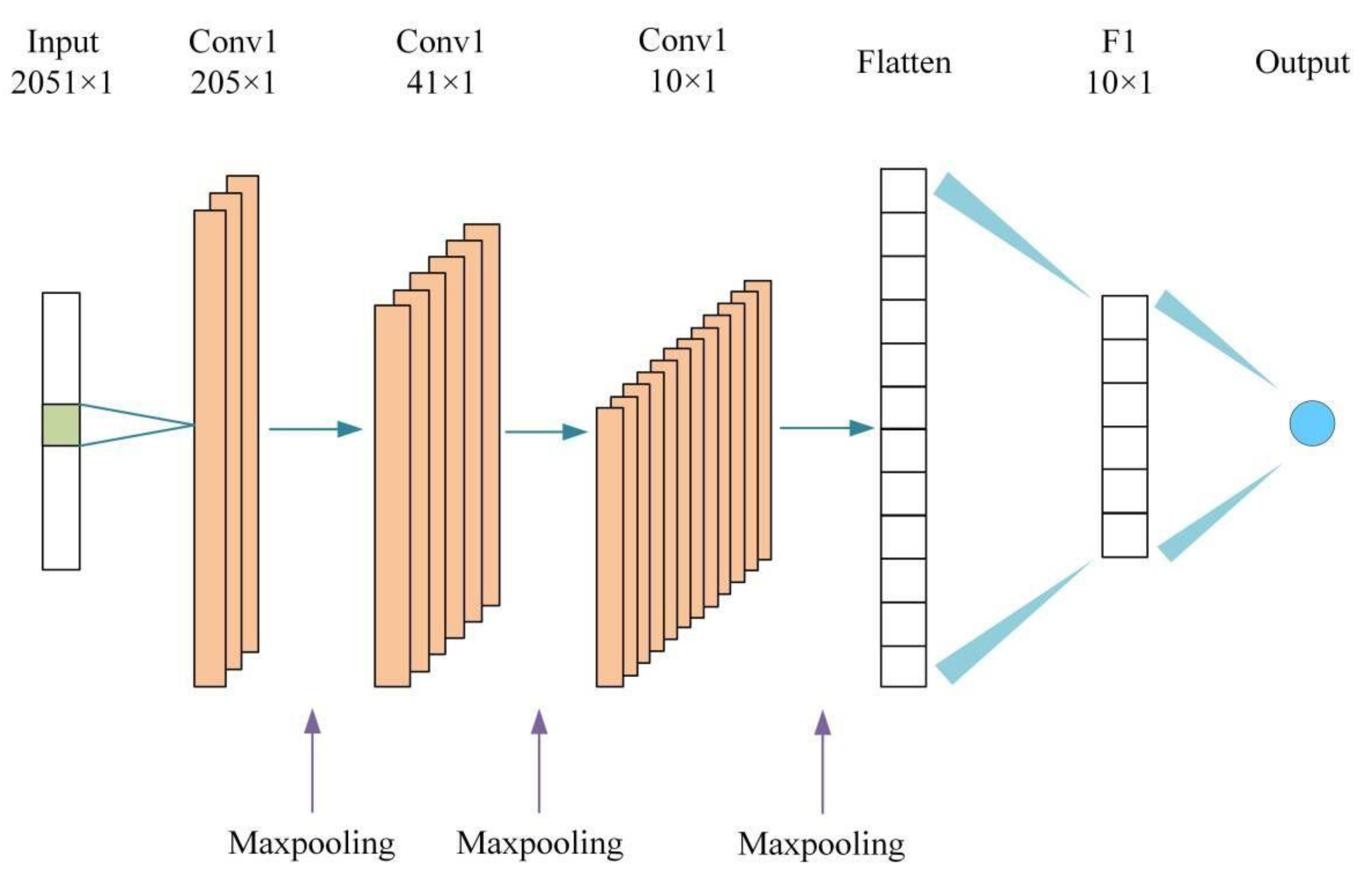
The 1D-CNN structure constructed in this study is shown in Figure 2. The input layer of the model uses the spectral data corresponding to the SOM, with 2051 data samples in total. The estimated values of the SOM content are used for the output layer. For this model, there are three convolutional layers (respectively labeled Conv1, Conv2 and Conv3), a flat layer (labeled Flatten), a fully connected layer (labeled F1) and an output layer. The hyperparameters set in this model are shown in Table 1. The specific settings are as follows: the optimizer is adam, the learning rate is 0.00005, and the number of iterations is 1000. The numbers of filters for the three convolutional layers are 5, 10 and 20, respectively. The stride size of the convolution layer is 1, and the stride size of each pooling layer is 2. The Relu function was chosen as the activation function.

2.6. Model Accuracy Evaluation

The estimation accuracy and stability of the model were determined using the coefficient of determination (R2), root mean square error (RMSE) and residual prediction deviation (RPD) together. The R2 characterizes the stability of a model, and the closer that R2 approaches 1, the more stable the model is and the better the fit. The RMSE reflects the difference between a valuation and a measured value, and the smaller the RMSE, the better the estimation ability of a model is. The RPD is the ratio of the sample standard deviation to the RMSE. When the RPD < 1.4, the estimation ability of the model is poor; 1.4 < RPD < 1.8 indicates fair estimation ability in a model, which could be used for rough estimation of SOM; 1.8 < RPD < 2.0 indicates a model with good estimation ability; 2.0 < RPD < 2.5 represents a very good estimation ability in a model; and RPD > 2.5 indicates excellent estimation ability in a model [46].

3. Results

3.1. Descriptive Statistics for Soil Organic Matter (SOM) Content

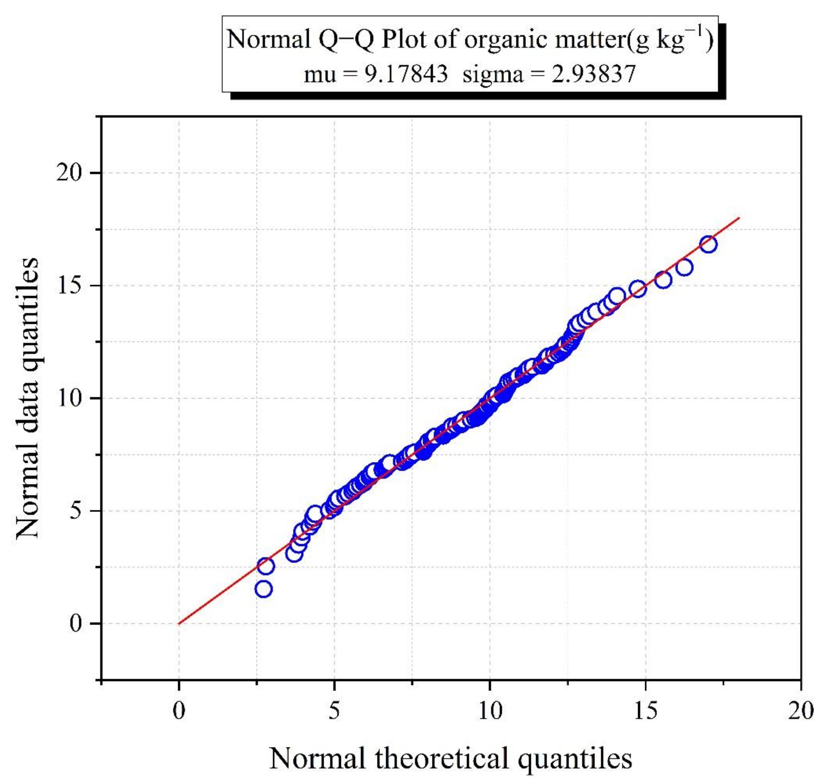
To improve the accuracy of model estimation, the 135 samples were divided into calibration and validation sets in a ratio of 2:1 in accordance with the Kennard–Stone algorithm [47]. As can be seen from Figure 3, the 135 soil samples were normally distributed. Most of the samples were distributed along the diagonal line, except for some slight deviations for individual samples. As seen in Table 2, both the total sample and the modeling set had SOM contents that ranged from 2.72 to 18.18 g kg−1, while the validation set had SOM content that ranged from 2.80 to 17.02 g kg−1. The average value of the 135 samples was less than 10.00 g kg−1, indicating a low organic matter content compared to the mean value of the global soil spectral library (21.60 g kg−1) [48]. The SOM content range of the validation set was narrower than those of the total sample set and the calibration set, which ensured that the SOM content of the validation set samples did not exceed the range of the estimated model. The coefficients of variation for the total sample set, calibration set and validation set were 32.87%, 32.94% and 32.91%.

3.2. Feature Variable Selected by PSO, ACO and SA algorithms

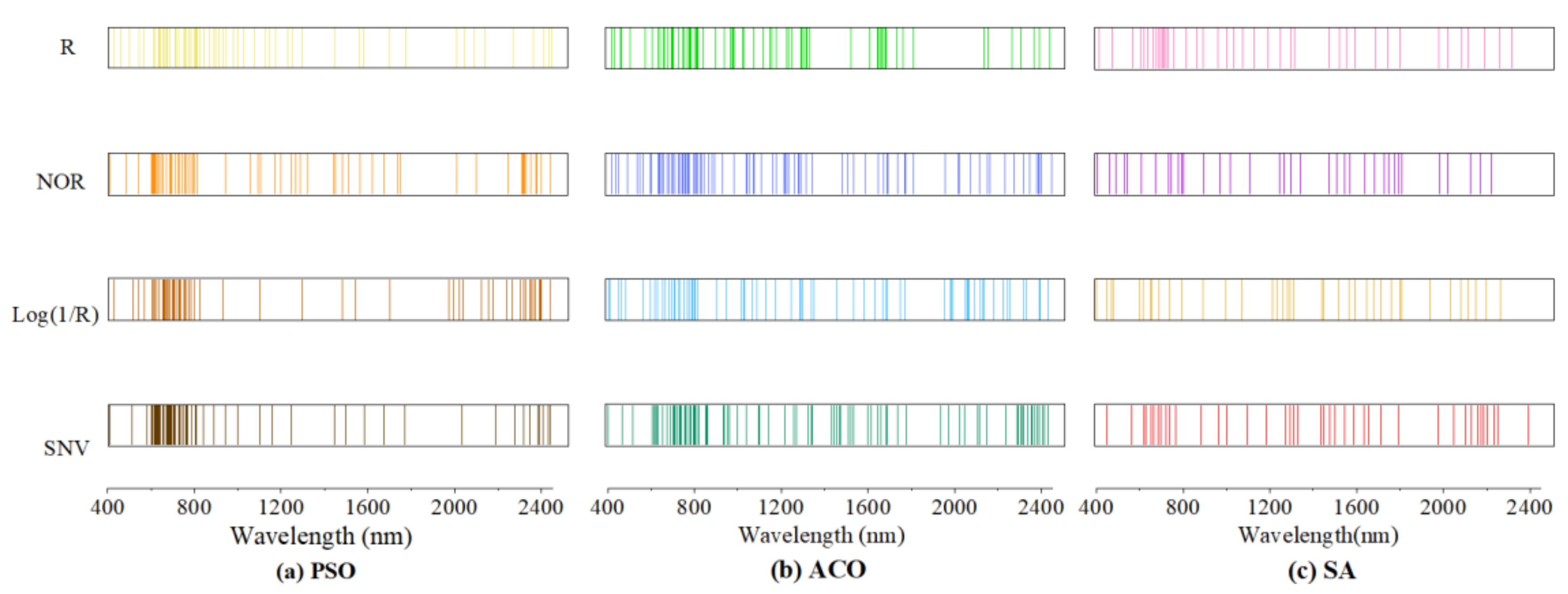
In order to screen out the characteristic bands of SOM that were less influenced by environmental factors, we used three characteristic variable selection methods, the PSO, ACO, and SA algorithms, to select the characteristic bands of SOM for the raw spectral data (R) and three pre-processed spectral datasets (SNV, Log(1/R) and NOR), and the feature variable selection results are shown in Figure 4. The R, SNV, Log(1/R) and NOR were screened using the PSO, ACO, and SA algorithms, and the number of bands screened out was more than 90% of the total. Among them, ACO retained about 71–93 of the characteristic bands, PSO selected 63–65 and SA selected 36–42 of the characteristic bands. The proportion of characteristic bands distributed in the 600–800 nm range was the largest (38.1%) with PSO and the smallest with SA (20%).
On the whole, the bands screened by the three band-selection methods were mainly located in the 600–800 nm range, and no spectral response bands with SOM were selected near 1400 nm and 1900 nm, and a large number of studies have shown that the vicinity around 1400 nm and 1900 nm is the band that is more affected by moisture [49]. Therefore, the characteristic variable selection method can effectively be used to select the characteristic bands associated with SOM with less external environmental influence.

3.3. Estimation Accuracy for SOM with Different Models and Validation

Table 3 shows the results from comparing the accuracy of the PLSR, BPNN and CNN models established using the SOM content with the corresponding full-band spectral data, as well as the characteristic bands screened by the different methods. Compared with R, the accuracy of the model estimation after SNV, NOR and Log (1/R) preprocessing was improved to different degrees, with the accuracy of the model that used SNV processing being the highest, with R2, RPD and RMSE values up to 0.71, 1.67 and 1.88 g kg−1. For all three feature variable selection methods, the estimation accuracy of the model established based on the characteristic band outperformed the full-band spectral data (400–2450 nm) modeling for both the validation and calibration sets. In particular, the SNV-PSO method obtained characteristic band modeling with 64 modeling variables, only accounting for 3.40% of the full band, but achieved the best stability for the SOM estimation model. The ranking of the three methods’ ability to improve the model accuracy had the following order: PSO > ACO > SA.
The ranking of the estimation accuracy of the three modeling methods for SOM content was in the order CNN > BPNN > PLSR. In the PLSR model, only the model developed with the characteristic bands screened by PSO could provide a rough estimate of SOM with an RPD between 1.4 and 1.49. The method based only on the SNV-ACO and PSO-selected characteristic bands in the BPNN model was capable of providing a rough estimate of SOM (1.4 < RPD < 1.8). All the models constructed with CNN could estimate the SOM content, except for the model constructed with full-band spectral data, which could not effectively estimate the SOM content. Among them, the SNV-PSO-CNN (R2 = 0.71, RPD = 1.67, RMSE = 1.88 g kg−1) model had the best estimation for quantitative estimation of SOM.
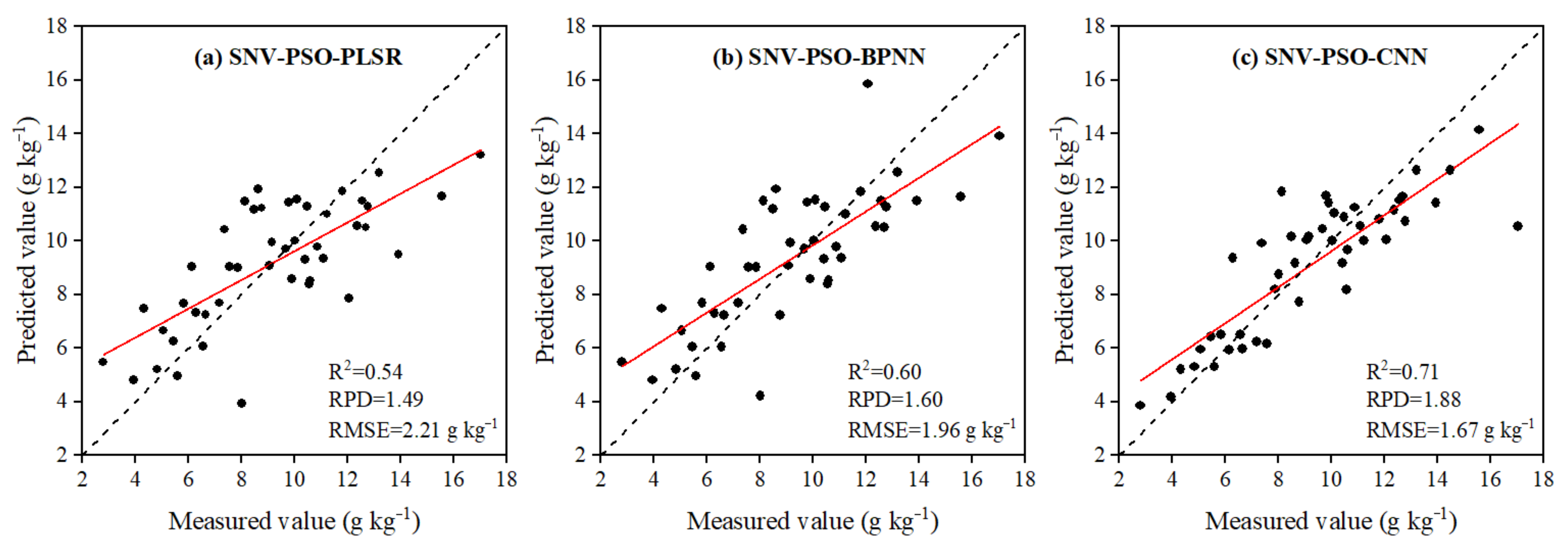
Comparing the evaluation parameters of the PLSR, BPNN and CNN models, it could be seen that the three modeling methods all attained the highest accuracy levels among the models built with PSO combined with SNV preprocessing screening of the characteristic bands (Figure 5). In this case, the actual and estimated values with SNV-PSO-CNN were closer to the 1:1 line, and the model accuracy was higher. Compared with SNV-PSO-PLSR and SNV-PSO-BPNN, the R2 and RPD values for the validation set were improved by 0.17 and 0.39 and 0.11 and 0.28, respectively, and the RMSE values were reduced by 0.54 g kg−1 and 0.29 g kg−1, respectively.

4. Discussion

4.1. The Factors Affecting the Prediction of SOM with Vis-NIR In Situ Hyperspectral Data

The estimation efficiency for SOM can be improved by using Vis-NIR in situ spectroscopy compared to indoor spectroscopy, but there is a loss in model accuracy due to the influence of environmental factors on the spectra in the field. This is attributed to the fact that Vis-NIR in situ spectroscopy measurements are influenced by factors such as soil moisture content, atmospheric water vapor, light intensity variations and soil surface roughness [50,51]. Waiser et al. found that the estimation accuracy of models constructed using laboratory spectra for air-dried, unground soil samples was higher than that of in situ spectral models for moist soils, indicating that soil moisture is an important factor suppressing the model prediction accuracy [52]. Hutengs et al. achieved high-precision estimation of soil organic carbon in soil samples with relatively dry air and soil moisture content between 1.50 and 16.80% [53]. However, the study area was located in Aksu in northwestern China, where water is scarce and soil is relatively dry. The moisture content of the collected soil samples ranged from 1.13% to 15.67%. October, during the dry season, was chosen as the sampling time, which further served to avoid the effect of soil moisture. The roughness of the soil surface also affects the soil spectral reflectance when measuring in situ spectra, which in turn affects the accuracy of SOM estimation. Wu et al. revealed that soil surface roughness and unevenness caused a partial loss of soil reflectance, resulting in a decrease in the measured soil spectral reflectance, consequently affecting the accuracy of SOM estimation [54]. Numerous studies have shown that the interference caused by soil roughness on spectral acquisition is relatively limited when a relatively homogeneous area of the surface is selected for measurement when determining in situ spectra [53,55]. Therefore, sites with relatively flat surfaces and no vegetation cover were selected for sample collection and Vis-NIR in situ spectroscopy measurements in this study. In addition, the presence of atmospheric water vapor also affects Vis-NIR in situ spectroscopy measurements. Bishop et al. identified the band near 1400 nm and 1900 nm as the band where moisture has a strong influence [49]. As influenced by atmospheric water vapor, light and other environmental effects, the spectral reflectance near 1400 nm and 1900 nm was more than 1 when measuring in situ spectral data in the field in this study, which greatly affected the inversion accuracy for SOM. However, this study used three methods to screen the characteristic bands of SOM and found that no spectral variables were screened near 1400 nm and 1900 nm. Consequently, the use of the PSO, ACO, and SA algorithms could effectively remove the effects of noise and environmental factors and improve the performance of models with Vis-NIR in situ spectral data in estimating SOM.

4.2. The Effect of Feature Variable Selection Algorithms on Model Accuracy

Existing studies have shown that SOM estimation models developed using characteristic bands can reduce data redundancy and improve the efficiency of data analysis [56,57]. The CARS and GA have achieved relatively good results as common feature variable selection algorithms [18]. However, the CARS and GA showed poor effects in this study due to the special soil conditions in south Xinjiang, where salinization is more serious. Therefore, three methods, the PSO, ACO, and SA algorithms, were selected for this study, and the characteristic bands were selected to establish a model for estimation of SOM and compared with the model constructed from full-band spectral data. As the results showed, the accuracy of the SOM estimation model developed using the characteristic bands was higher than that of the model established by the full-band spectral data. This was attributed to the fact that the feature variable selection method can effectively filter out unrelated spectral information, retain the effective spectral information and reduce the signal-to-noise ratio, thus improving the model estimation accuracy. The selected spectral variables of the three methods in this study were mainly focused around 600–800 nm. This region is an important spectral response band for SOM, as has been demonstrated by numerous studies [19,27,58]. Analysis of the model evaluation metrics comparing the three modeling approaches revealed that, regardless of the modeling approach, the PSO-based model had the highest accuracy, ACO second highest and SA the worst. Li et al. also observed high accuracy for the model built based on bands selected by the PSO [59], which is consistent with the conclusions obtained in this study. We believe that SA has the worst prediction accuracy because of the lowest number of remaining characteristic bands, over-excluding some of the spectral variables related to SOM. Although ACO selected the most spectral variables, the model accuracy was lower than that of PSO, which may have been due to the interference of redundant information in the spectral variables selected by ACO.

4.3. Influence of the Different Modeling Methods on the SOM Prediction Accuracy

When building a model for hyperspectral estimation of SOM, the influence on the determination of soil spectra varies across different geographic regions. Therefore, it is difficult to establish a model for estimating SOM content suitable for all regions [60]. In this paper, we analyzed and compared the evaluation metrics of the constructed models and found that the model built with the CNN was better than those with BPNN and PLSR in estimating SOM content, which is the same conclusion obtained by Khosravi et al. [61]. The PLSR, which is a classical linear model, can solve the linear problem well, but the SOM and the corresponding spectral variables are not simply linear. Therefore, it is difficult to fully explain the complex nonlinearity between SOM and spectral variables using PLSR, and there are limitations [62]. The BPNN has a strong nonlinear mapping capability that can better simulate the relationship between SOM and spectral reflectance; however, because of the large amount of data obtained with hyperspectral techniques, the BPNN has a limited ability to handle complex relationships between bands, which greatly reduces the accuracy and efficiency of the estimation of SOM content [63]. In contrast, the CNN, as the earliest proposed deep learning model, has better model estimation capabilities than traditional models, with deeper network layers and stronger feature extraction capabilities, and it can dig out the important information contained in the spectrum, simplify the computational procedure and improve the model estimation accuracy [64]. This study demonstrated that SNV-PSO-CNN is the optimal combined model for estimating SOM. However, this study is a regional study, and the applicability of models varies from region to region due to differences in soil texture, soil water content and the external environment [65]. Therefore, the conclusions obtained in this study can provide research ideas for the study of soil properties in different regions, and further research is needed to explore whether this model is applicable to other regions.

5. Conclusions

In this study, three feature variable selection methods—the particle swarm algorithm (PSO), ant colony algorithm (ACO) and simulated annealing (SA)—were used to extract characteristic bands by combining the original spectral data and three pre-processed spectral datasets, using three modeling methods—partial least squares (PLSR), the back propagation neural network (BPNN) and the convolutional neural network (CNN)—to establish the inversion model for SOM based on Vis-NIR in situ spectra. The ranking of the estimation accuracy of the three modeling methods for SOM content was in the order CNN > BPNN > PLSR. Compared to the models constructed from full-band spectral data, all three feature selection methods could improve the accuracy of SOM estimation, but PSO showed the most significant improvement. In addition, the CNN model developed with SNV combined with PSO selection of characteristic bands was the optimal model for estimating SOM (R2 = 0.71, RPD = 1.88, RMSE = 1.67 g kg−1), providing a good estimation of SOM content and an effective method for monitoring SOM in desert areas using in situ Vis-NIR spectroscopy.

Author Contributions

All authors contributed in a substantial way to the manuscript. Methodology, J.H. and P.Y.; formal analysis, D.L. and P.Y.; data curation, P.Y.; writing—original draft preparation, P.Y.; writing—review and editing, J.P.; conceptualization, J.H.; investigation, P.Y.; project administration, J.P.; funding acquisition, J.P.; visualization, B.H. All authors have read and agreed to the published version of the manuscript.

Funding

This research was supported by grants from the Tarim University President’s Fund (grant nos TDZKCX202205 and TDZKSS202227), the National Key Research and Development Program of China (grant nos. 2018YFE0107000) and the National Science Foundation of China (grant nos. 42071068, 41061031 and 42201073).

Institutional Review Board Statement

Not applicable.

Informed Consent Statement

Not applicable.

Data Availability Statement

Not applicable.

Conflicts of Interest

The authors declare no conflict of interest.

References

  1. De Santana, F.B.; de Giuseppe, L.O.; de Souza, A.M.; Poppi, R.J. Removing the moisture effect in soil organic matter determination using NIR spectroscopy and PLSR with external parameter orthogonalization. Microchem. J. 2019, 145, 1094–1101. [Google Scholar] [CrossRef]
  2. McBratney, A.; Field, D.J.; Koch, A. The dimensions of soil security. Geoderma 2014, 213, 203–213. [Google Scholar] [CrossRef] [Green Version]
  3. Lehmann, J.; Kleber, M. The contentious nature of soil organic matter. Nature 2015, 528, 60–68. [Google Scholar] [CrossRef] [PubMed]
  4. Muhammad, S.; Müller, T.; Joergensen, R.G. Decomposition of pea and maize straw in Pakistani soils along a gradient in salinity. Biol. Fert. Soils 2006, 43, 93–101. [Google Scholar] [CrossRef]
  5. Xu, S.; Zhao, Y.; Wang, M.; Shi, X. Comparison of multivariate methods for estimating selected soil properties from intact soil cores of paddy fields by Vis–NIR spectroscopy. Geoderma 2018, 310, 29–43. [Google Scholar] [CrossRef]
  6. Liu, Y.; Liu, Y.; Chen, Y.; Zhang, Y.; Shi, T.; Wang, J.; Hong, Y.; Fei, T.; Zhang, Y. The influence of spectral pretreatment on the selection of representative calibration samples for soil organic matter estimation using Vis-NIR reflectance spectroscopy. Remote Sens. 2019, 11, 450. [Google Scholar] [CrossRef] [Green Version]
  7. Bao, N.; Wu, L.; Ye, B.; Yang, K.; Zhou, W. Assessing soil organic matter of reclaimed soil from a large surface coal mine using a field spectroradiometer in laboratory. Geoderma 2017, 288, 47–55. [Google Scholar] [CrossRef]
  8. Rossel, R.V.; McBratney, A.B. Soil chemical analytical accuracy and costs: Implications from precision agriculture. Aust. J. Exp. Agric. 1998, 38, 765–775. [Google Scholar] [CrossRef]
  9. Jiang, Q.; Chen, Y.; Guo, L.; Fei, T.; Qi, K. Estimating soil organic carbon of cropland soil at different levels of soil moisture using VIS-NIR spectroscopy. Remote Sens. 2016, 8, 755. [Google Scholar] [CrossRef] [Green Version]
  10. Selige, T.; Böhner, J.; Schmidhalter, U. High resolution topsoil mapping using hyperspectral image and field data in multivariate regression modeling procedures. Geoderma 2006, 136, 235–244. [Google Scholar] [CrossRef]
  11. Nocita, M.; Kooistra, L.; Bachmann, M.; Müller, A.; Powell, M.; Weel, S. Predictions of soil surface and topsoil organic carbon content through the use of laboratory and field spectroscopy in the Albany Thicket Biome of Eastern Cape Province of South Africa. Geoderma 2011, 167, 295–302. [Google Scholar] [CrossRef] [Green Version]
  12. Swierenga, H.; De Groot, P.J.; De Weijer, A.P.; Derksen, M.W.J.; Buydens, L.M.C. Improvement of PLS model transferability by robust wavelength selection. Chemometr. Intell. Lab. Syst. 1998, 41, 237–248. [Google Scholar] [CrossRef]
  13. Swierenga, H.; Wülfert, F.; De Noord, O.E.; De Weijer, A.P.; Smilde, A.K.; Buydens, L.M.C. Development of robust calibration models in near infra-red spectrometric applications. Anal. Chim. Acta. 2000, 411, 121–135. [Google Scholar] [CrossRef]
  14. Galvão, R.K.H.; Araújo, M.C.U.; Silva, E.C.; José, G.E.; Soares, S.F.C.; Paiva, H.M. Cross-validation for the selection of spectral variables using the successive projections algorithm. J. Am. Chem. Soc. 2007, 18, 1580–1584. [Google Scholar] [CrossRef]
  15. Zou, X.; Zhao, J.; Povey, M.J.; Holmes, M.; Mao, H. Variables selection methods in near-infrared spectroscopy. Anal. Chim. Acta 2010, 667, 14–32. [Google Scholar]
  16. Shi, T.; Chen, Y.; Liu, H.; Wang, J.; Wu, G. Soil organic carbon content estimation with laboratory-based visible–near-infrared reflectance spectroscopy: Feature selection. Appl. Spectrosc. 2014, 68, 831–837. [Google Scholar] [CrossRef]
  17. Xu, S.; Zhao, Y.; Wang, M.; Shi, X. Determination of rice root density from Vis–NIR spectroscopy by support vector machine regression and spectral variable selection techniques. Catena 2017, 157, 12–23. [Google Scholar] [CrossRef]
  18. Xie, S.; Ding, F.; Chen, S.; Wang, X.; Li, Y.; Ma, K. Prediction of soil organic matter content based on characteristic band selection method. Spectrochim. Acta A Mol. Biomol. Spectrosc. 2022, 273, 120949. [Google Scholar] [CrossRef]
  19. Hong, Y.; Chen, Y.; Yu, L.; Liu, Y.; Liu, Y.; Zhang, Y.; Liu, Y.; Cheng, H. Combining fractional order derivative and spectral variable selection for organic matter estimation of homogeneous soil samples by VIS–NIR spectroscopy. Remote Sens. 2018, 10, 479. [Google Scholar] [CrossRef] [Green Version]
  20. Xie, S.; Li, Y.; Wang, X.; Liu, Z.; Ma, K.; Ding, L. Research on estimation models of the spectral characteristics of soil organic matter based on the soil particle size. Spectrochim. Acta A Mol. Biomol. Spectrosc. 2021, 260, 119963. [Google Scholar] [CrossRef]
  21. Sun, W.; Liu, S.; Zhang, X.; Li, Y. Estimation of soil organic matter content using selected spectral subset of hyperspectral data. Geoderma 2022, 409, 115653. [Google Scholar] [CrossRef]
  22. Bai, Z.; Xie, M.; Hu, B.; Luo, D.; Wan, C.; Peng, J.; Shi, Z. Estimation of Soil Organic Carbon Using Vis-NIR Spectral Data and Spectral Feature Bands Selection in Southern Xinjiang, China. Sensors 2022, 22, 6124. [Google Scholar] [CrossRef]
  23. Mahesh, S.; Jayas, D.S.; Paliwal, J.; White, N.D.G. Comparison of partial least squares regression (PLSR) and principal components regression (PCR) methods for protein and hardness predictions using the near-infrared (NIR) hyperspectral images of bulk samples of Canadian wheat. Food Bioprocess Technol. 2015, 8, 31–40. [Google Scholar] [CrossRef]
  24. Wold, S.; Ruhe, A.; Wold, H.; Dunn, W.J., III. The collinearity problem in linear regression. The partial least squares (PLS) approach to generalized inverses. SIAM. J. Sci Comput. 1984, 5, 735–743. [Google Scholar] [CrossRef] [Green Version]
  25. Wijewardane, N.K.; Ge, Y.; Morgan, C.L. Moisture insensitive prediction of soil properties from VNIR reflectance spectra based on external parameter orthogonalization. Geoderma 2016, 267, 92–101. [Google Scholar] [CrossRef] [Green Version]
  26. Cheng, H.; Wang, J.; Du, Y. Combining multivariate method and spectral variable selection for soil total nitrogen estimation by Vis–NIR spectroscopy. Arch. Agron. Soil Sci. 2021, 67, 1665–1678. [Google Scholar] [CrossRef]
  27. Liu, H.; Zhang, Y.; Zhang, B. Novel hyperspectral reflectance models for estimating black-soil organic matter in Northeast China. Environ. Monit. Assess. 2009, 154, 147–154. [Google Scholar] [CrossRef] [PubMed]
  28. Ng, W.; Minasny, B.; Montazerolghaem, M.; Padarian, J.; Ferguson, R.; Bailey, S.; McBratney, A.B. Convolutional neural network for simultaneous prediction of several soil properties using visible/near-infrared, mid-infrared, and their combined spectra. Geoderma 2019, 352, 251–267. [Google Scholar] [CrossRef]
  29. LeCun, Y.; Bengio, Y.; Hinton, G. Deep learning. Nature 2015, 521, 436–444. [Google Scholar] [CrossRef]
  30. Xu, Z.; Zhao, X.; Guo, X.; Guo, J. Deep learning application for predicting soil organic matter content by VIS-NIR spectroscopy. Comput. Intell. Neurosci. 2019, 2019, 3563761. [Google Scholar] [CrossRef]
  31. World Reference Base for Soil Resources. International Soil Classification System For naming Soils and Creating Legends for Soil Maps; Food and Agriculture Organization of the United Nations: Rome, Italy, 2014. [Google Scholar]
  32. Peng, J.; Biswas, A.; Jiang, Q.; Zhao, R.; Hu, J.; Hu, B.; Shi, Z. Estimating soil salinity from remote sensing and terrain data in southern Xinjiang Province, China. Geoderma 2019, 337, 1309–1319. [Google Scholar] [CrossRef]
  33. Liang, Z.; Chen, S.; Yang, Y.; Zhao, R.; Shi, Z.; Rossel, R.A.V. National digital soil map of organic matter in topsoil and its associated uncertainty in 1980’s China. Geoderma 2019, 335, 47–56. [Google Scholar] [CrossRef]
  34. Ji, W.; Li, S.; Chen, S.; Shi, Z.; Rossel, R.A.V.; Mouazen, A.M. Prediction of soil attributes using the Chinese soil spectral library and standardized spectra recorded at field conditions. Soil Tillage Res. 2016, 155, 492–500. [Google Scholar] [CrossRef]
  35. De Santis, R.; Montanari, R.; Vignali, G.; Bottani, E. An adapted ant colony optimization algorithm for the minimization of the travel distance of pickers in manual warehouses. Eur. J. Oper. Res. 2018, 267, 120–137. [Google Scholar] [CrossRef]
  36. Liu, J.; Ma, X.; Li, X.; Liu, M.; Shi, T.; Li, P. Random convergence analysis of particle swarm optimization algorithm with time-varying attractor. Swarm. Evol. 2021, 61, 100819. [Google Scholar] [CrossRef]
  37. Kirkpatrick, S.; Gelatt, C.D., Jr.; Vecchi, M.P. Optimization by simulated annealing. Science 1983, 220, 671–680. [Google Scholar] [CrossRef]
  38. Siarry, P.; Berthiau, G.; Durdin, F.; Haussy, J. Enhanced simulated annealing for globally minimizing functions of many-continuous variables. ACM Trans. Math. Softw. 1997, 23, 209–228. [Google Scholar] [CrossRef]
  39. Hörchner, U.; Kalivas, J.H. Further investigation on a comparative study of simulated annealing and genetic algorithm for wavelength selection. Anal. Chim. Acta 1995, 311, 1–13. [Google Scholar] [CrossRef]
  40. Araújo, S.R.; Wetterlind, J.; Dematte, J.A.M.; Stenberg, B. Improving the prediction performance of a large tropical vis-NIR spectroscopic soil library from Brazil by clustering into smaller subsets or use of data mining calibration techniques. Eur. J. Soil Sci. 2014, 65, 718–729. [Google Scholar] [CrossRef]
  41. Morellos, A.; Pantazi, X.E.; Moshou, D.; Alexandridis, T.; Whetton, R.; Tziotzios, G.; Wiebensohn, J.; Bill, R.; Mouazen, A.M. Machine learning based prediction of soil total nitrogen, organic carbon and moisture content by using VIS-NIR spectroscopy. Biosyst. Eng. 2016, 152, 104–116. [Google Scholar] [CrossRef] [Green Version]
  42. Wang, L.; Zeng, Y.; Chen, T. Back propagation neural network with adaptive differential evolution algorithm for time series forecasting. Expert Syst. Appl. 2015, 42, 855–863. [Google Scholar] [CrossRef]
  43. Kavzoglu, T.; Mather, P.M. The use of backpropagating artificial neural networks in land cover classification. Int. J. Remote Sens. 2003, 24, 4907–4938. [Google Scholar] [CrossRef]
  44. LeCun, Y.; Bottou, L.; Bengio, Y.; Haffner, P. Gradient-based learning applied to document recognition. Proc. IEEE 1998, 86, 2278–2324. [Google Scholar] [CrossRef] [Green Version]
  45. Qu, J.L.; Yu, L.; Yuan, T.; Tian, Y.; Gao, F. Adaptive fault diagnosis algorithm for rolling bearings based on one-dimensional convolutional neural network. Chin. J. Sci. Instrum. 2018, 39, 134–143. [Google Scholar]
  46. Gholizadeh, A.; Žižala, D.; Saberioon, M.; Borůvka, L. Soil organic carbon and texture retrieving and mapping using proximal, airborne and Sentinel-2 spectral imaging. Remote Sens. Environ. 2018, 218, 89–103. [Google Scholar] [CrossRef]
  47. Kennard, R.W.; Stone, L.A. Computer aided design of experiments. Technometrics 1969, 11, 137–148. [Google Scholar] [CrossRef]
  48. Viscarra Rossel, R.A.; Behrens, T.; Ben-Dor, E.; Brown, D.J.; Demattê, J.A.M.; Shepherd, K.D.; Shi, Z.; Stenberg, B.; Stevens, A.; Adamchuk, V. A global spectral library to characterize the world’s soil. Earth-Sci. Rev. 2016, 155, 198–230. [Google Scholar] [CrossRef] [Green Version]
  49. Bishop, J.L.; Lane, M.D.; Dyar, M.D.; Brown, A.J. Reflectance and emission spectroscopy study of four groups of phyllosilicates: Smectites, kaolinite-serpentines, chlorites and micas. Clay Miner. 2008, 43, 35–54. [Google Scholar] [CrossRef]
  50. Christy, C.D. Real-time measurement of soil attributes using on-the-go near infrared reflectance spectroscopy. Comp. Electron. Agric. 2008, 61, 10–19. [Google Scholar] [CrossRef]
  51. Rinnan, Å.; Van Den Berg, F.; Engelsen, S.B. Review of the most common pre-processing techniques for near-infrared spectra. Trends Anal. Chem. 2009, 28, 1201–1222. [Google Scholar] [CrossRef]
  52. Waiser, T.H.; Morgan, C.L.; Brown, D.J.; Hallmark, C.T. In situ characterization of soil clay content with visible near-infrared diffuse reflectance spectroscopy. Soil Sci. Soc. Am. J. 2007, 71, 389–396. [Google Scholar] [CrossRef]
  53. Hutengs, C.; Seidel, M.; Oertel, F.; Ludwig, B.; Vohland, M. In situ and laboratory soil spectroscopy with portable visible-to-near-infrared and mid-infrared instruments for the assessment of organic carbon in soils. Geoderma 2019, 355, 113900. [Google Scholar] [CrossRef]
  54. Wu, C.Y.; Jacobson, A.R.; Laba, M.; Baveye, P.C. Accounting for surface roughness effects in the near-infrared reflectance sensing of soils. Geoderma 2009, 152, 171–180. [Google Scholar] [CrossRef]
  55. Stevens, A.; van Wesemael, B.; Bartholomeus, H.; Rosillon, D.; Tychon, B.; Ben-Dor, E. Laboratory, field and airborne spectroscopy for monitoring organic carbon content in agricultural soils. Geoderma 2008, 144, 395–404. [Google Scholar] [CrossRef] [Green Version]
  56. Lao, C.; Chen, J.; Zhang, Z.; Chen, Y.; Ma, Y.; Chen, H.; Ma, Y.; Chen, H.; Gu, X.; Ning, J.; et al. Predicting the contents of soil salt and major water-soluble ions with fractional-order derivative spectral indices and variable selection. Comp. Electron. Agric. 2021, 182, 106031. [Google Scholar] [CrossRef]
  57. Li, H.; Liang, Y.; Xu, Q.; Cao, D. Key wavelengths screening using competitive adaptive reweighted sampling method for multivariate calibration. Anal. Chim. Acta 2009, 648, 77–84. [Google Scholar] [CrossRef]
  58. Wu, Y.; Chen, J.; Ji, J.; Gong, P.; Liao, Q.; Tian, Q.; Ma, H. A mechanism study of reflectance spectroscopy for investigating heavy metals in soils. Soil Sci. Soc. Am. J. 2007, 71, 918–926. [Google Scholar] [CrossRef]
  59. Li, L.; Zhang, Y.; Fung, J.C.; Qu, H.; Lau, A.K. A coupled computational fluid dynamics and back-propagation neural network-based particle swarm optimizer algorithm for predicting and optimizing indoor air quality. Build. Environ. 2022, 207, 108533. [Google Scholar] [CrossRef]
  60. Chen, Y.; Wang, J.; Liu, G.; Yang, Y.; Liu, Z.; Deng, H. Hyperspectral estimation model of forest soil organic matter in northwest Yunnan Province, China. Forests 2019, 10, 217. [Google Scholar] [CrossRef] [Green Version]
  61. Khosravi, V.; Ardejani, F.D.; Yousefi, S.; Aryafar, A. Monitoring soil lead and zinc contents via combination of spectroscopy with extreme learning machine and other data mining methods. Geoderma 2018, 318, 29–41. [Google Scholar] [CrossRef]
  62. Liu, F.; Jiang, Y.; He, Y. Variable selection in visible-near infrared spectra for linear and nonlinear calibrations: A case study to determine soluble solids content of beer. Anal. Chim. Acta 2009, 635, 45–52. [Google Scholar] [CrossRef] [PubMed]
  63. Yuan, Q.; Shen, H.; Li, T.; Li, Z.; Li, S.; Jiang, Y.; Xu, H.; Tan, W.; Yang, Q.; Wang, J.; et al. Deep learning in environmental remote sensing: Achievements and challenges. Remote. Sens. Environ. 2020, 241, 111716. [Google Scholar] [CrossRef]
  64. Zhang, M.; Zhao, Z. Near Infrared Spectral Analysis Modeling Method Based on Deep Belief Network. Spectrosc. Spect. Anal. 2020, 40, 2512. [Google Scholar]
  65. Zhang, Z.; Ding, J.; Zhu, C.; Wang, J.; Ma, G.; Ge, X.; Li, Z.; Han, L. Strategies for the efficient estimation of soil organic matter in salt-affected soils through Vis-NIR spectroscopy: Optimal band combination algorithm and spectral degradation. Geoderma 2021, 382, 114729. [Google Scholar] [CrossRef]
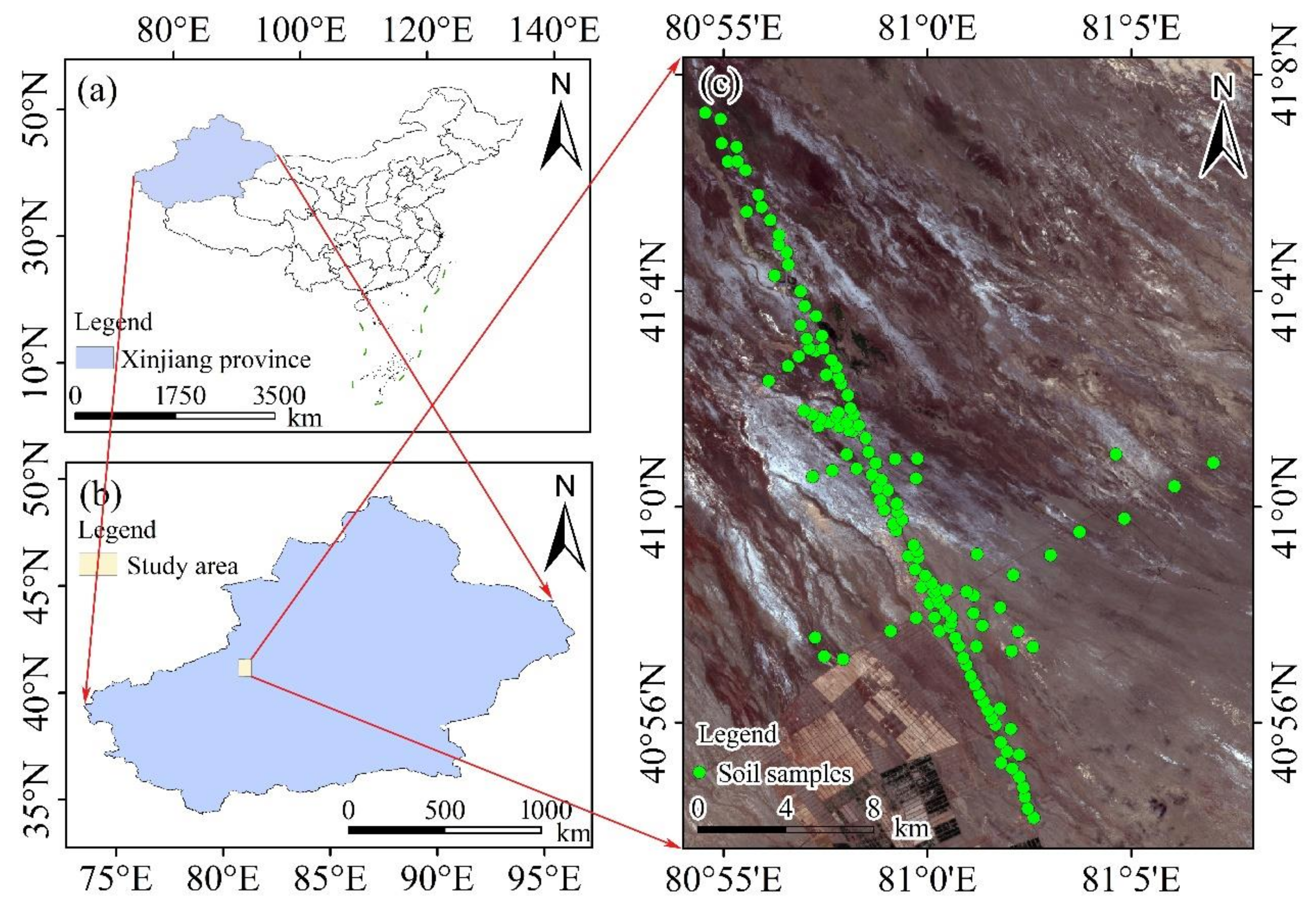
Figure 1. The geographical locations of Xinjiang province, China (a), and the study area (b) and the spatial distribution of the sampling points (c).
Remotesensing 14 05221 g001
Figure 2. The CNN structure of the SOM estimation model.
Remotesensing 14 05221 g002
Figure 3. Q−Q plot for organic matter.
Remotesensing 14 05221 g003
Figure 4. The distributions of characteristic bands with different feature variable selection algorithms. (a) the characteristic bands of SOM screened by particle swarm algorithm; (b) the characteristic bands screened by ant colony algorithm; and (c) the characteristic bands screened by simulated annealing algorithm.
Remotesensing 14 05221 g004
Figure 5. Scatter plots of measured versus estimated SOM contents based on PLSR (a), BPNN (b) and CNN models (c) combined with PSO and SNV (for validation dataset). The solid red and gray lines in each plot represent the regression line and 1:1 line, respectively.
Remotesensing 14 05221 g005
Table 1. Hyperparameter settings in the deep learning SOM estimation model.
HyperparameterValues
Kernel size 110
Kernel size 25
Kernel size 34
Batch size11
Dropout layer0.5
Max. epochs1000
Learning rate0.00005
Learning rate decay0.001
Table 2. Descriptive statistics for soil organic matter (g kg−1).
DatasetNumberMeanMin aMax bSD cCV d (%)
Calibration909.382.7218.183.0932.94
Validation459.362.8017.023.0832.91
Total1359.372.7218.183.0832.87
Note: a minimum; b maximum; c standard deviation; d coefficient of variation.
Table 3. Cross-validation for of the PLSR, BPNN and CNN calibration models for the spectral datasets and the SOM (g kg−1).
ModelSpectral PretreatmentsVariable NumberCalibrationValidation
R2RMSER2RMSERPD
PLSRR20510.352.510.342.541.24
SNV20510.452.350.422.461.28
Log(1/R)20510.422.410.402.491.26
NOR20510.382.440.372.531.24
R-PSO630.532.210.512.191.41
SNV-PSO640.591.810.542.121.49
Log(1/R)-PSO630.522.150.532.141.43
NOR-PSO650.502.250.482.211.40
R-ACO710.452.460.432.501.27
SNV-ACO920.482.390.492.301.35
Log(1/R)-ACO750.472.410.452.471.30
NOR-ACO930.492.310.472.401.31
R-SA410.442.450.432.401.31
SNV-SA420.462.370.452.381.32
Log(1/R)-SA380.442.460.412.481.29
NOR-SA360.432.480.422.431.30
BPNNR20510.372.400.362.531.25
SNV20510.482.000.452.421.29
Log(1/R)20510.442.120.432.471.28
NOR20510.412.250.392.481.27
R-PSO630.581.830.562.171.45
SNV-PSO640.621.740.601.961.60
Log(1/R)-PSO630.591.820.572.101.50
NOR-PSO650.551.950.542.191.43
R-ACO710.512.000.472.421.30
SNV-ACO920.541.940.552.201.43
Log(1/R)-ACO750.531.960.502.291.36
NOR-ACO930.551.920.522.251.40
R-SA410.472.110.452.391.32
SNV-SA420.492.010.472.381.33
Log(1/R)-SA380.452.130.432.411.30
NOR-SA360.442.230.442.401.31
CNNR20510.392.440.382.521.27
SNV20510.471.870.462.391.32
Log(1/R)20510.461.890.442.421.30
NOR20510.441.920.422.481.27
R-PSO630.651.650.641.871.69
SNV-PSO640.731.510.711.671.88
Log(1/R)-PSO630.681.640.661.841.71
NOR-PSO650.631.690.621.941.63
R-ACO710.551.860.542.201.45
SNV-ACO920.661.520.631.891.67
Log(1/R)-ACO750.621.550.582.001.57
NOR-ACO930.611.690.601.971.60
R-SA410.531.860.542.211.44
SNV-SA420.591.610.572.151.46
Log(1/R)-SA380.551.820.522.251.40
NOR-SA360.531.850.532.241.42
Publisher’s Note: MDPI stays neutral with regard to jurisdictional claims in published maps and institutional affiliations.