Article

Geostatistical Modelling of Soil Spatial Variability by Fusing Drone-Based Multispectral Data, Ground-Based Hyperspectral and Sample Data with Change of Support

by
Antonella Belmonte
1,
Carmela Riefolo
2,*,
Francesco Lovergine
1 and
Annamaria Castrignanò
3
1
Institute for Electromagnetic Sensing of the Environment, National Research Council (CNR-IREA), Via Amendola 122/D, 70126 Bari, Italy
2
CREA-AA—Council for Agricultural Research and Economics, Via Celso Ulpiani, 5, 70125 Bari, Italy
3
Department of Engineering and Geology (InGeo), Gabriele D’Annunzio University of Chieti-Pescara, 66013 Chieti, Italy
*
Author to whom correspondence should be addressed.
Remote Sens. 2022, 14(21), 5442; https://doi.org/10.3390/rs14215442
Submission received: 7 October 2022 / Revised: 24 October 2022 / Accepted: 25 October 2022 / Published: 29 October 2022
(This article belongs to the Special Issue Topsoil Characterization by Means of Remote Sensing)

Abstract

:
Traditional soil characterization methods are time consuming, laborious and invasive and do not allow for long-term repeatability of measurements. The overall aim of this paper was to assess and model spatial variability of the soil in an olive grove in south Italy by using data from two sensors of different types: a multi-spectral on-board drone radiometer and a hyperspectral visible-near infrared-shortwave infrared (VIS-NIR-SWIR) reflectance radiometer, as well as sample data, to arrive at a delineation of homogeneous areas. The hyperspectral data were processed using Continuum Removal (CR) methodology to obtain information about the content and composition of clay. Differently, the multispectral data were firstly upscaled to the support of soil data using geostatistics and taking into account the change of support. Secondly, the data acquired with the two different sensors were integrated with soil granulometric properties by using two multivariate geostatistical techniques: multi-collocated cokriging to achieve a more exhaustive and finer-scale soil characterization, and multi-collocated factor cokriging to extract synthetic scale-dependent indices (regionalized factors) for the delineation of soil in homogeneous zones. This paper shows the impact of change of support on the uncertainty of soil prediction that can have a significant effect on decision making in Precision Agriculture. Moreover, four regionalized factors at two different scales (two for each scale) were retained and mapped. Each factor provided a different delineation of the field with areas characterized by different granulometries and clay compositions. The applied method is sufficiently flexible and could be applied to any number and type of sensors.

1. Introduction

In recent years, agriculture has been undergoing a profound revolution, moving from an era characterized by widespread mechanization to an intensive use of information [1,2] such as Precision Agriculture (PA) [3]. Agriculture is currently much more complex than in the past, and its success depends strongly on the efficiency and reliability of the methods used to collect site-specific within-field information and to process this large amount of data.
Among the various components of an agricultural system, soil is undoubtedly one of the most important due to its significant impact on plant growth, yield and product quality/safety [2,3,4]. Farmers have always been well aware of this, since for centuries, they have been using soil information to make their agronomic management decisions. Traditionally, soil information has been collected with grid sampling at both regional and local scales. While this method has produced useful results in the past, it currently shows all its limitations in modern agriculture, having its disadvantages. The information obtained with sampling is generally expensive and inevitably sparse, i.e., it is not available at every point in the field. To make informed management decisions in agriculture, it is necessary to have soil information at more detailed scales, sometimes even at sub-metric scales for certain agricultural operations such as pathogen control [5] and weed detection [6], which would make grid sampling almost impractical.
Fortunately, modern technology offers several opportunities to make effective use of the massive amount of data made available to the farmer today. However, appropriate data processing techniques are needed to integrate the limited soil information from sampling with the higher spatial density information provided by remote (RS) and proximal (PS) sensing.
These are two techniques that acquire the information about an object without physical contact (case RS) either in direct contact or at a maximum height of 2 m from the surface (case PS). The RS uses distinct platforms as satellites, airborne or UAV with different sensors. Instead, the PS are mounted on platforms ranging from handheld, fixed installations, or robotics and tractor-embedded [7] sensors. Many studies have used RS images of bare soil and soil reflectance to map and quantitatively characterize soil attributes [8,9,10,11,12], although these remotely sensed data cannot be considered as a substitute for direct soil sampling and lab measurements. A more efficient way of considering soil data acquired by RS is to see them as a new, complementary and valuable source of soil information to provide more precise predictions [11,12,13].
Moreover, images of bare soil from satellite or aircraft can cover large areas with a sufficient degree of detail, to allow for the estimation of some key properties of the soil, even where ground samplings could be considered sparse by traditional soil surveyors [8]. Although the technical characteristics of satellite products have improved a lot in recent years, such as those commercially offered by EOS (Earth Observation System, ww.eos.com (accessed on 24 October 2022)), their spatial resolution may not be adequate in PA.
To improve the predictions of crop yield models based on aerial images of the plant at one meter or tens of meters scale, there is need to supplement them with soil data at least at a similar scale [14,15,16]. Furthermore, in order to be able to intervene promptly with some agronomic operation, there is need to have an on-time record of the state of the crop and/or soil. Aerial measurements from a drone (UAV) make it possible to obtain images of soil or crop at a centimetric spatial resolution and at the time desired by the farmer. This explains the increasing use of drones for PA in recent times also in combination with lower prices and fewer restrictions on flight authorization.
Although the use of hyperspectral radiometers on board drones is becoming increasingly popular, it is currently not yet common in PA, due to both the still high costs and the complexity of signal processing. Multispectral images with low spectral density may sometimes limit interpretation of spatial variability of soil properties.
Furthermore, spectroscopic reflectance measurements on soil samples obtained in the laboratory allow for quantitative determinations of soil properties. It has now become common laboratory practice for soil analytical measurements. However, hyperspectral data captured with spectrometers are generally noisy and difficult to interpret even under well-controlled laboratory conditions [2,17,18]. It is therefore extremely critical to use appropriate procedures for both data pre-processing and analysis. Currently three distinct estimation techniques are widely applied to characterize qualitative and quantitative soil attributes: (1) chemometric techniques by regression models as partial least square regression (PLSR) models [19]; (2) machine learning techniques [20] widely used in recent years, and (3) continuum removal (CR) [21].
While pre-treatment methods are required to correct baseline shifts in reflectance spectra across the wavelength range due to the scattering effect [22,23], CR is a normalization treatment of spectra which only concerns those absorption regions to be compared against a common baseline [24]. This technique has the advantage of identifying specific absorption features that should persist at different observation conditions.
After the application of the CR method, intensity values of absorption at specific bands can be calculated from VNIR-SWIR spectra to estimate minerals, rocks and some soil properties. The absorption characteristics of several minerals, including clay and CaCO3, have been extensively studied using this technique both under laboratory conditions [25] and from remotely sensed data [26]. New machine learning techniques are being developed but to determine mainly the main chemical and physical properties of soil such as organic carbon, clay and pH [20].
Soil samples for lab spectroscopic analysis are usually collected with grid sampling, which inevitably limits their number.
After this brief examination of the potential and limitations of the different methods of measurement, it is evident that there is no single sensor capable of providing accurate measurements of all soil properties. To improve the accuracy of spatial predictions, a successful approach may be used for several different sensors in addition to direct laboratory measurements of soil attributes, a process called data fusion [27,28,29]. The fusion of sensors allows the inputs from different sensors to be combined synergistically into a single image of the environment/soil under study [30,31,32,33,34,35].
The resulting model is more accurate because it balances the strengths of the different sensors. It is then possible to use the information provided by sensor fusion to support more informed actions. This is by no means a trivial problem since it involves jointly analysing heterogeneous multi-source spatial data with different statistical properties and spatial resolution [34,35]. Furthermore, when delineating management zones in PA, predictions are made at a higher level of spatial association than the one of the original data (upscaling). This process, known as change of support [36,37,38], reduces spatial heterogeneity and estimate uncertainty by producing a smoothing effect. Geostatistics offers various solutions to data fusion and change of support problems specifically in PA. Block cokriging for modelling spatial variability and block factor cokriging for partitioning field into homogeneous sub-field areas are the traditional geostatistical techniques used to treat these critical issues. The advantages of using geostatistics derive from the fact that it explicitly takes into account the spatial correlation between observations and allows the reduction in uncertainty, due to upscaling, to be evaluated quantitatively.
The objective of this work is the definition of a geostatistical approach of multi-spectral drone soil data fusion with hyperspectral ground-based data and laboratory granulometry measurements for field delineation in homogeneous areas, which is also capable of estimating the uncertainty reduction due to scale change.

2. Materials and Methods

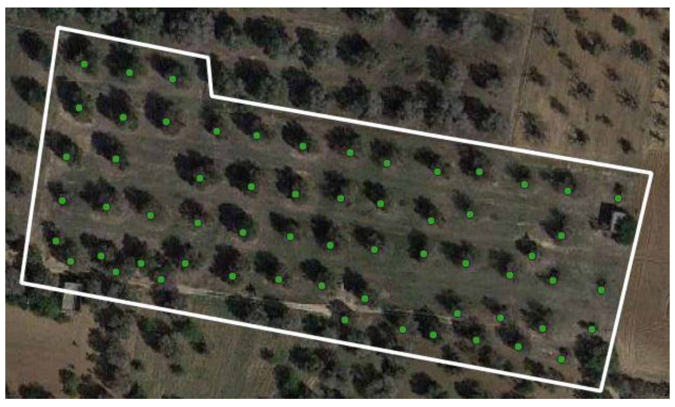
2.1. Soil Sampling and Study Site

The sampling was carried out in an olive grove of 100-year-old trees of the Ogliarola Salentina cultivar in July 2019, located in Oria (province of Brindisi, southeast of Italy). Topsoil (0–0.20 m) subsamples were collected in three different places under each of the 61 plants of the olive grove field, with a sampling scale of 16 m on average. The sampling design was therefore determined by the particular geometry of the olive grove planting. Since the soil was compact, we dug with a spade a small vertical-walled hole to the chosen depth. Then, we took a vertical slice covering the entire layer, trying to keep a constant weight of the sample (about 2 kg). This operation was repeated for each of the three subsamples. Finally, they were placed on a clean plastic tarp and mixed to form a composite sample and stored in a plastic bag. The sampling design (Figure 1) is formed by centroids of plants, around which (at about 1 m) the soil was taken. It was chosen because one objective of the project was also to investigate whether the occurrence of xylella infection might change the properties of the soil surrounding the plant. The distance between trees was of 15 m on average.
The field is flat and gravel free. The inter-plant soil remains dry and free of weeds for long periods in summer due to drought. It is classified as Calcic Haploxeralf, fine, mixed, thermic (USDA, 1999), which is widespread in Mediterranean areas where grapes and olives are cultivated. The term “Haploxeralf” involves a loamy granulometry and a relatively thin argillic or kandic horizon, whereas “Calcic” regards a calcic horizon with its upper boundary within 1 m of the mineral soil surface. Since in this study a topsoil (0–0.20 m) was surveyed, this characteristic is not quite relevant.

2.2. Drone Data

The images were acquired from a multispectral sensor mounted on a multi-rotor DJI Mavic Pro drone in August 2019 when most of the soil was free of weeds. The platform had a total payload mass of ~800 g and a flight range of ~7 km [31,35]. The camera (Parrot Sequoia) allowed for acquiring multispectral images at high resolution (0.07 m) from an altitude of 70 m and with a sampling distance (GSD) of 0.066 m/pixel. The high spatial resolution was required because this study was part of a research project aimed at early detection of olive plants affected by Xylella [29].
The characteristics of the multispectral sensor are reported in the Table 1.
The acquisitions were performed using the typical aerial-mapping “serpentine” profile (Figure 2a) with planned overlap and 80% sidelap.
All of the spectral data sets were processed with Pix4d Mapper 4.4.12 software applying photogrammetric techniques, to create a quoted point cloud for 3D reconstruction and an orthophoto image for each band as the final result (Figure 2b).
The drone image had previously been classified into three classes (crown, shadow and soil) [35]. The classification product was then cut using the polygon shapefile of the field boundary (Oria-RE). In the following, there is the description of the different steps of the applied methodology for extracting soil pixels alone from the drone image:
  • Recombining classes and mask generation
In this step, the procedure ‘combine classes’ of the commercial ENVI (ENvironment for Visualizing Images) 5.1 software (Harris Geospatial) was applied. In this way, two classes (crown and shadow) were merged into one class ‘not-soil’, and then, the corresponding binary image (not soil 0, soil 1) was extracted.
2.
Point shapefile of soil
Four point shapefiles containing soil information were extracted from each drone band using the tool (r.tovector) of the Grass (Geographic Resources Analysis Support System) module integrated in the open source software: QGIS (Quantum Geographic Information System) version 3.22, Białowieża, Poland.
3.
CSV file
To use soil drone data in the subsequent geostatistical analysis, the point shapefile was converted into CSV format. This step was performed by applying the plugin MMQGIS in QGIS.
The methodology to extract the soil information from drone data is shown in the following flowchart (see Figure 3).

2.3. Laboratory-Based Granulometry Measurement

The granulometric determinations were based on taking the suspension of particles with diameters less than 200 µm at different heights and at predetermined times according to the pipette method [39,40]. The following soil particle size fractions (%) were determined directly: coarse sand (2.0–0.2 mm), silt (0.05–0.002 mm) and clay (<0.002 mm). The fine sand (0.2–0.05 mm) was calculated as the complement to 100 of the previous components. Total sand was calculated as the sum of coarse and fine sand.

2.4. Hyperspectral Data and Their Analysis

The three soil samples, collected under the 61 plants, were dried, ground, sieved to 2 mm and mixed to compose a representative, homogeneous soil sample for each tree. They were analysed in the laboratory with ASD FieldSpec IV spectroradiometer (Analytical Spectral Devices Inc., Boulder, CO, USA) over 350–2500 nm spectral range, and VIS-NIR-SWIR reflectance was measured.
The raw data over the whole spectral range were elaborated with principal component analysis in a previous paper [31], and the retained components (PCs) were elaborated with continuum removal [41] in the ranges around 1400, 1900, 2200 nm, to assess the influence of clay composition illite (1400 nm), montmorillonite (1900 nm), kaolinite (2200 nm) [24] on PCs’ structure. As described in the paper of Riefolo et al., 2022 [31], the three retained PCs cumulatively explained a proportion of the variance greater than 98%; more particularly, PC1 explained the 92.2%, PC2 4% and PC3 2% of total variance. Significant loading values were those above a threshold level of 80. PC1 had significant loadings around 1400 nm and from 1710 to 1810 nm. Between these two wavelength ranges, the one most directly associable to a clay component was 1400 nm (illite), according Dufrechou et al., 2015 [41]. Given the high percentage of total variance explained, PC1 could be interpreted as a kind of average soil reflectance over the entire spectrum explored. PC2 showed significant loadings in the ranges between 1970 and 1990 nm and at 2500 nm; therefore, it could be associated with the montmorillonite component [41]. Finally, PC3, showing significant loadings in the 370–440 nm range, was associated with iron oxides and more specifically with geothite.
One of the objectives of this paper was not only to estimate the granulometric components of soil but also to characterize the composition of the clay. Due to the fact that soil is a complex system comprising several different substances and not a pure mineral, it is likely that other water-containing components may affect the spectra at some specified wavelengths, although the samples were desiccated in the laboratory. To make it comparable, the depth parameters previously calculated at 1400 nm (D1400) and at 1900 nm (D1900) were standardized with respect to the parameter depth at 2200 m (D2200) [41]. Therefore, the following ratios: R1 = D1400/D2200 and R2 = D1900/D2200, were calculated and were related spatially to other soil variables, regarding the particular granulometry discussed in this paper.

2.5. Spectral Index of Soil Samples

In order to characterize, using only one index, the spectral properties of a soil sample provided by the hundreds of spectral bands of the ASD sensor, a discrimination measure was used, called SID-SAM, which is a mixture of the widely used RS spectral angle mapper (SAM) and the spectral information divergence (SID) [31,32,33,34,35,36,37,38,39,40,41,42].
It is a stochastic measure of discrimination between two spectra and therefore is well suited to be interpolated according to the techniques of geostatistics. To make the values referring to the 61 soil samples comparable to each other, these measurements were determined with respect to the same spectrum, corresponding to the maximum reflectance for all samples over the entire spectrum (Figure 4).
In Figure 4, the characteristic absorption bands at 1400, 1900 and 2200 nm are also visible in all spectra of soil samples, mainly assignable to the presence of illite, montmorillonite and kaolinite, respectively.

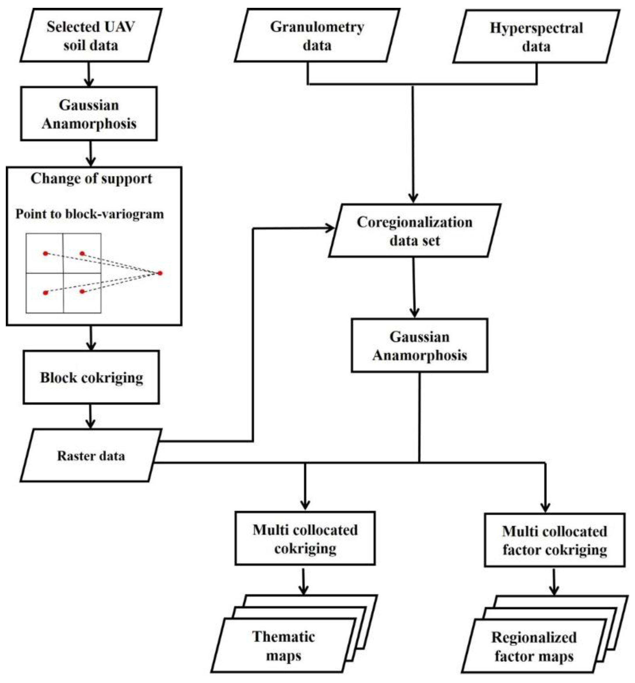
2.6. Geostatistical Procedures

Firstly, exploratory data analysis was performed to calculate the basic statistics of the study variables including mean, median, minimum and maximum values, standard deviation, skewness and kurtosis.
If the data distributions appeared asymmetrical with a skewness coefficient greater than 1, the variables were transformed into standardized Gaussian variables with mean 0 and variance 1, before performing multivariate geostatistical analysis. For this purpose, a Hermite polynomial series was used, and the approach is called Gaussian Anamorphosis [43,44].
Therefore, all geostatistical procedures were performed in the Gaussian domain, and only the end the estimates were back-transformed to the raw data by using the fitted anamorphosis model.
The multivariate data sets, both the one containing only drone data and the combined one resulting from the fusion of multi-band drone data, hyperspectral data and soil granulometric measurements, were spatially modelled under the scope of the linear model of coregionalization (LMC) [43,45]. LMC considers the study variables as generated by the same independent physical processes acting over Ns different spatial scales. All experimental direct and cross-variograms were then jointly modelled as linear combinations of the same set of Ns basic variograms gu(h) for each spatial scale u standardized to sill 1:
γ i j ( h ) = u = 1 N s b i j u g u ( h ) i , j = 1 , , p
where γij(h) is the cross-variogram model between variables Zi and Zj; h is a distance vector, called lag, and b i j u are the partial sills of the variograms gu(h), specific for each pair of variables i and j and for each spatial scale u.
By assembling all b i j u coefficients related to a specific scale u, a symmetric Bu matrix is determined, which is called the coregionalization matrix. This could be considered as the analogue of the variance–covariance matrix but for a specific scale u. Therefore, according to the LMC perspective, the variance–covariance matrix could be decomposed into the sum of the coregionalization matrices relating to Ns spatial scales [46]. Fitting of LMC was performed with weighted least-squares method under the constraint of positive semi-definiteness of the Bu by using an iterative approach developed by Rivoirard (2001) [47]. The results were evaluated with cross-validation techniques [48] using mean and variance of the standardized error (SE) against the cokriging standard deviation as error statistics [49]. The optimal values of the two statistics should be 0 and 1, respectively.

2.7. Change of Support

Geostatistical techniques are used to model the statistical effects of change of scale when soil measurements are made on point support (soil cores, pits, etc.), but the estimates are to be calculated on blocks (support) bigger than the one of observations (field, land unit). This is obtained by modifying the spatial functions (covariance, variogram) that describe the spatial dependence between observations, thus avoiding a new soil survey [49,50,51]. This procedure in geostatistics is called regularization [44].
The change of support of the drone data was made necessary in order to fuse heterogeneous data (multi-band drone, hyperspectral and granulometric data) with different supports in the multivariate geostatistical analysis.
The point support was assumed to be that of multispectral drone data (0.07 m × 0.07 m), while the estimates were obtained on a 1 × 1 m block, because this was the support of the measurements on the ground (granulometry and hyperspectral reflectance). To transform the point variograms of the drone data into block variograms, each block of 1 by 1 m size of the interpolation grid was discretized into equal cells with mesh of 0.10 m. After that, pseudo-point experimental variograms were calculated in the fictitious cell centres within the block, and then, the point variograms were averaged (regularized) over the block.
To provide the estimates of multi-spectral drone data on a 1 by 1 m block support, block cokriging was applied, which is one of the traditional geostatistical interpolation methods to solve the change of support problem [44,52,53]. It allows one to predict the variables at a scale larger than the one of observation through the process of regularization as described before. Block support variograms of drone data were then calculated from point support variograms to provide mean estimates on a 1 m mesh grid [5]. Block cokriging allows one to refer the estimates of different variables to the same support (block), thus solving the crucial problem of combining sensor data with different spatial resolutions [33].

2.8. Data Fusion and Partitioning of the Field

2.8.1. Multi-Collocated Cokriging

Cokriging is the traditional multivariate estimator in geostatistics which enables one to improve the accuracy of poorly sampled variables by using more densely sampled auxiliary variables [54,55].
In particular, the variant multi-collocated cokriging was used in this work to fuse sparse primary variables with gridded auxiliary variables, with the aim of improving the spatial resolution of soil properties as compared to sampling resolution (tens of meters). Multi-collocated cokriging [27,47] is a simplified version of full cokriging, which makes use of the much more densely sampled auxiliary variable(s) only at the target point and at all locations where the primary variable(s) of interest is(are) available [56]. This approach requires that the auxiliary variable(s) is(are) known at all nodes of the interpolation grid besides at the locations where the interest variable(s) is(are) measured. It is particularly useful when the auxiliary variables are redundant (raster variables), whereby the use of the full neighbourhood for interpolation would cause the inversion of the matrices to be very time-consuming or even impossible [43,44].
In this work, the multi-band drone variables were first interpolated onto a 1 m mesh grid with block cokriging and then assumed as auxiliary grid variables in the application of multi-collocated cokriging and multi-collocated factor cokriging to the complete fusion data set.

2.8.2. Multi-Collocated Factor Cokriging

The same LMC fitted for the fusion data set was used in multi-collocated factorial cokriging analysis to extract few synthetic scale-dependent indicators to be used for field partition. Factor cokriging is a geostatistical technique for assessing and modelling the spatial correlations of a multivariate spatial data set at the different scales, developed by Matheron (1982) [57]. Besides LMC fitting, it consists of two additional steps: (i) analysing the correlation structure of variables at each scale by applying traditional principal component analysis (PCA) on the corresponding coregionalization matrix to extract a set of orthogonal components known as scale-dependent regionalized factors; and (ii) cokriging and mapping regionalized factors by solving a modified cokriging system [43]. The variant multi-collocated factor cokriging was used in the same manner as illustrated earlier. Regionalized factors are but mathematical constructions with no prior physical meaning [37]; therefore, they were interpreted on the basis of the prevalent loading coefficients in their formulation.
The proposed data fusion approach is depicted in the flowchart of Figure 5.

2.9. Estimation Uncertainty

Estimation uncertainty of the granulometric variables (silt, clay), which were the target variables of this work, was assessed by calculating the confidence interval (95% CI), which provides the range of variation of the estimate at each node of the interpolation grid with an error less than or equal to 5% [5]. The upper and lower 95% CI limits pertaining to the Gaussian estimate were calculated by summing or subtracting the 1.96 cokriging standard deviation to the estimate, respectively. Upper and lower limits and estimate of Gaussian-transformed variables were then back-transformed to the raw data by using the Gaussian anamorphosis model, previously fitted. This made it possible to calculate the estimation uncertainty of even strongly skewed variables.

3. Results and Discussion

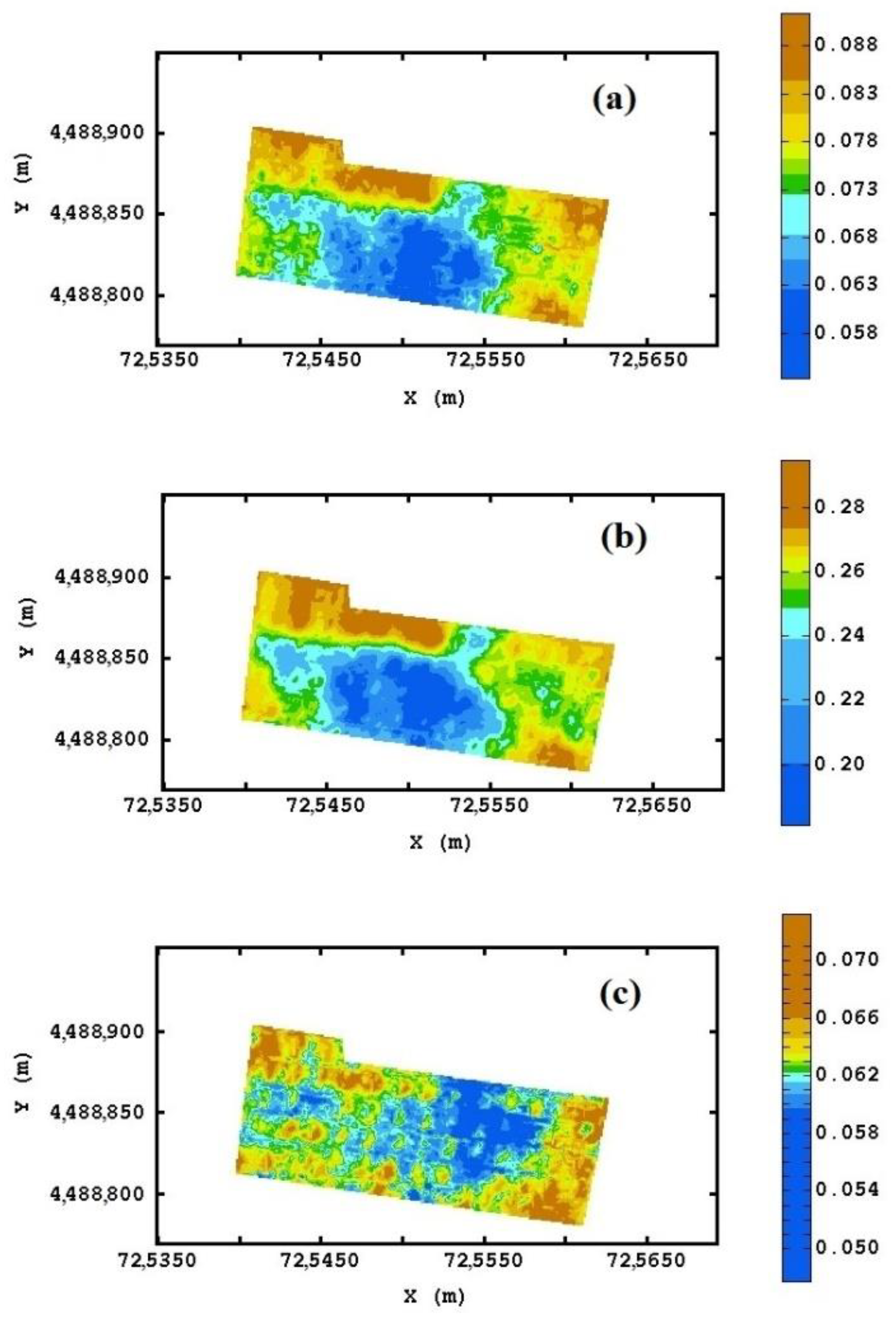
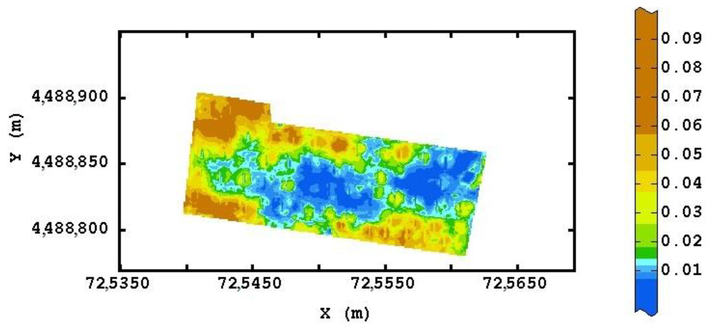
3.1. Geostatistical Analysis of Drone Data and Change of Support

From the original drone image, 2,032,972 pixels were extracted attributable to soil, and in Table 2, the basic statistics of the four bands of soil reflectance are reported. All four variables showed a skewness coefficient greater than 1, which means that the data distributions were asymmetric due to the presence of numerous large outliers.
Therefore, all four variables were transformed to standardized Gaussian variables by fitting a point model of Gaussian anamorphosis with a number of Hermite polynomials equal to 100. However, to calculate the set of experimental direct and cross-variograms of the Gaussian-transformed data in a workable computer time, it was necessary to reduce the number of pixels. This was realized by superimposing a regular grid with 1 m mesh on the study area and then randomly selecting one point within each cell, thus retaining 12,974 pixels. The LMC fitted to the set of experimental variograms of the transformed variables consisted of three basic spatial structures: a nugget effect, a spherical model with a range equal to 7.78 m, and a spherical model with a range of 76.59 m. The results of cross-validation (Table 3) were quite good because the mean and variance of the standardized error were very close to 0 and 1, respectively, for all variables.
By summing the structure-specific eigenvalues, it was possible to decompose the total spatial variance into three components accounting for 43%, (nugget effect), 43% (short-range) and 14% (long range). These results show a clear prevalence of the variability at short scales, within about 7 m, most likely due to the very fine scale (0.07 m) of drone data monitoring.
To fuse the drone data with the ground-based data with larger support (1 by 1 m), the experimental variograms were regularized on the larger support, and then, a block LMC was fitted (Figure 6) including a nugget effect, a spherical model with a range of 10.93 m, and a spherical model with a range of 77.59 m.
The percentages of total spatial variance explained by the three components were: 41% (nugget effect), 33% (short-range) and 26% (long-range). The effect of the change of support was therefore to leave LMC practically unchanged in the mathematical form of its basic structures, while the proportions of total variance explained by each component were varied. There was a proportional reduction in short-range variability in favour of long-range variability, although the error component (nugget effect) remained high. Differently, there was a significant reduction in the total spatial variance from 5.26 for the point model to 2.93 for the block model (about 56%), as it results from the sum of all respective eigenvalues.
Block LMC was then used in block cokriging to obtain the estimates of drone-transformed data both at the nodes of a 1 m-mesh grid (auxiliary grid data) and at the locations of the soil samples (sample data), in order to create the complete coregionalization data set including all variables used in data fusion.

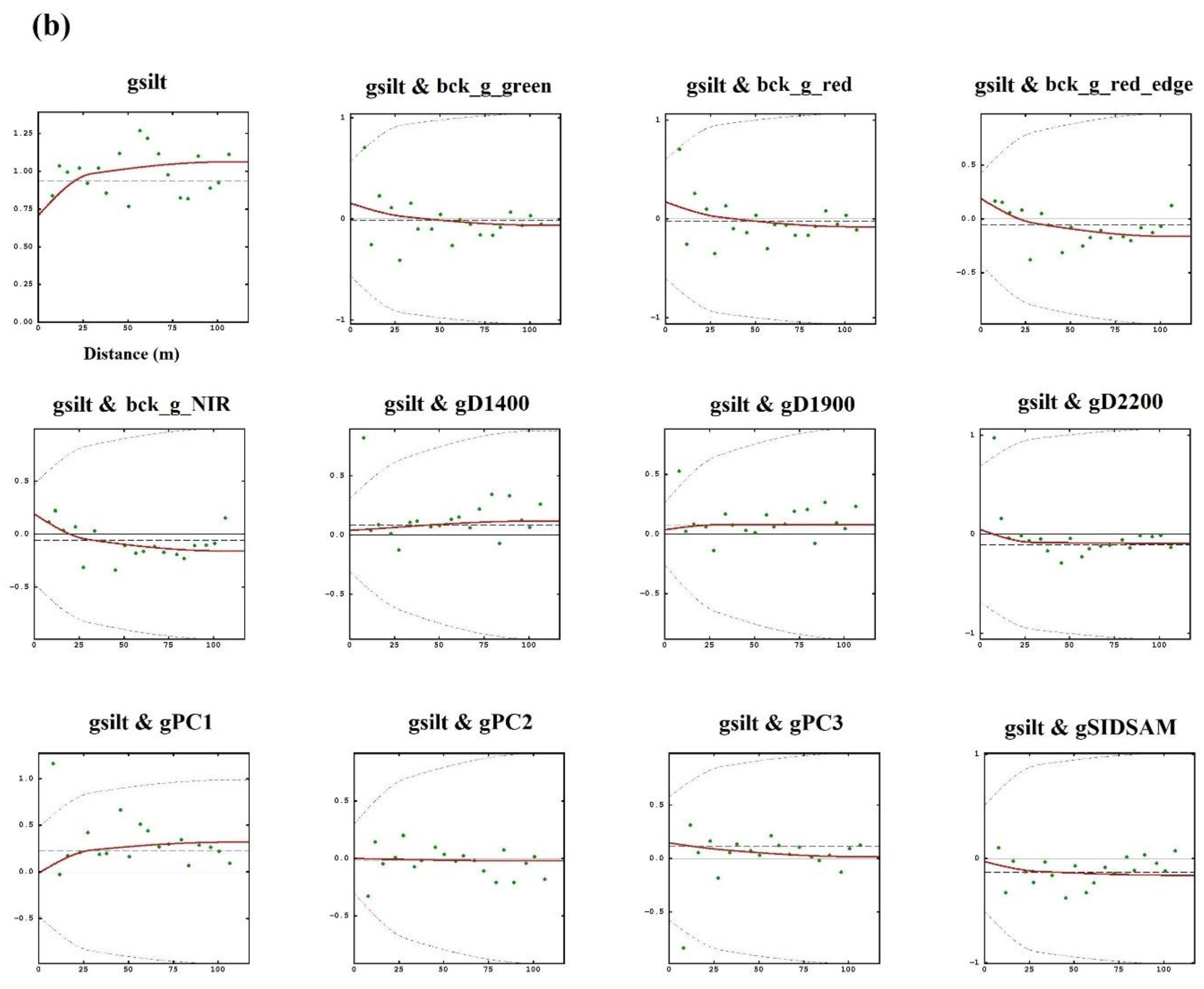
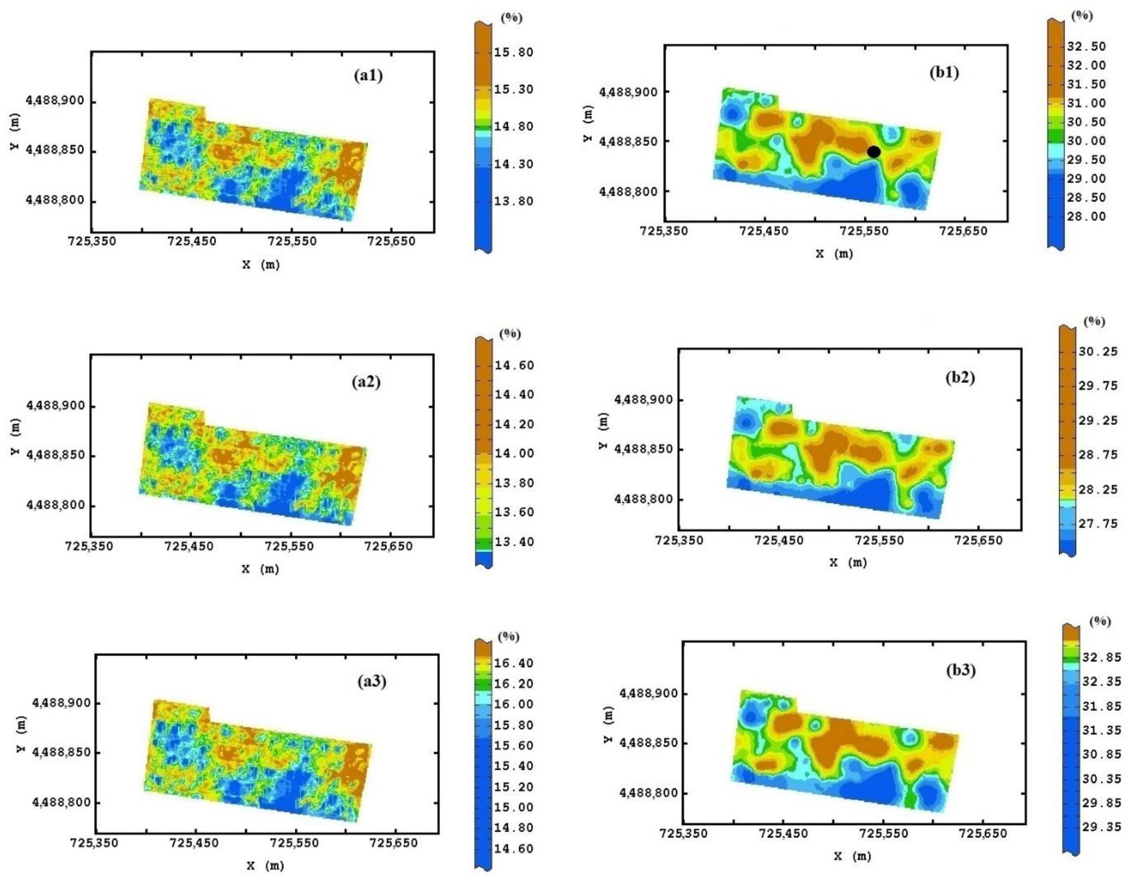
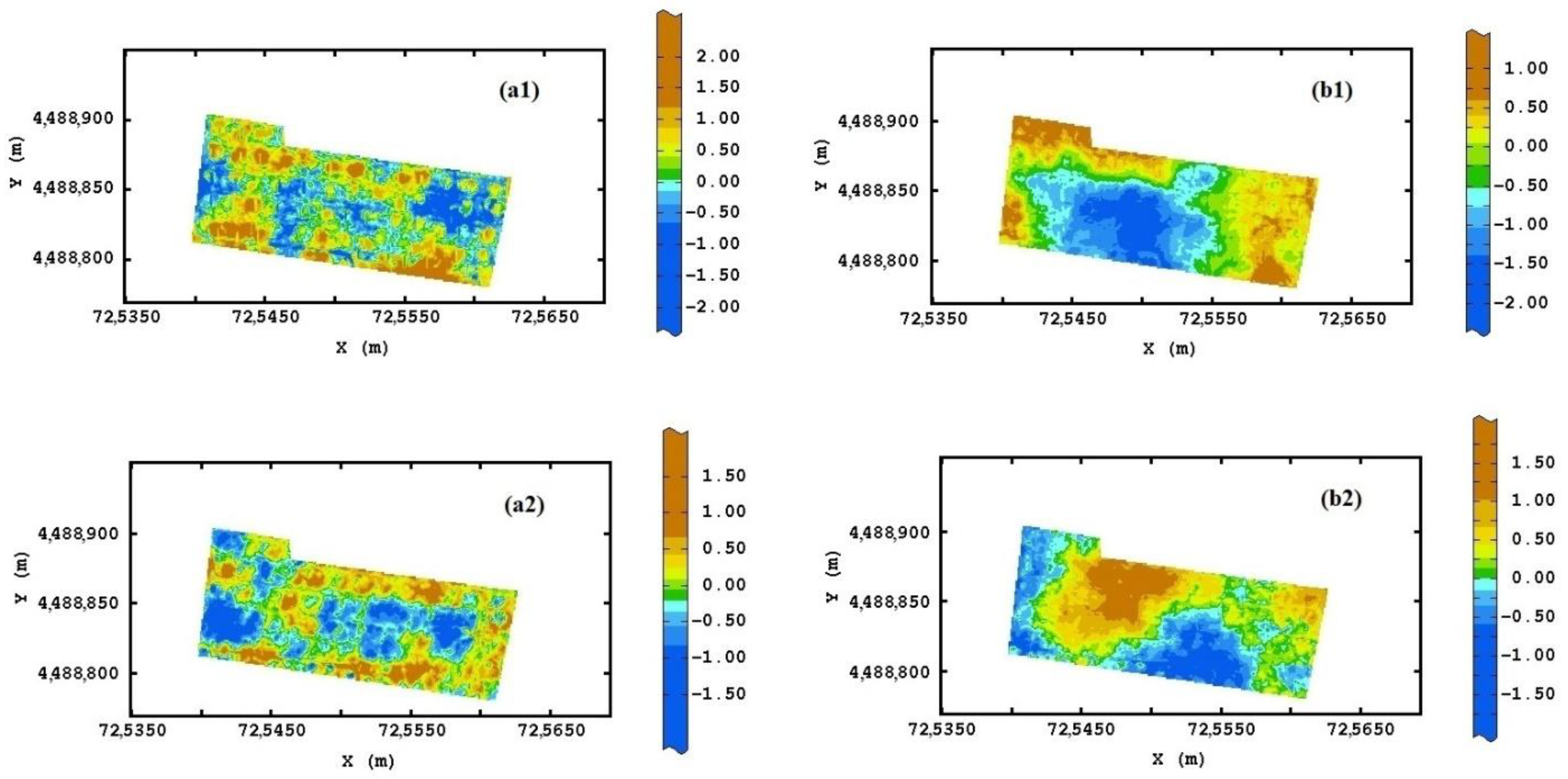
3.2. Geostatistical Soil Data Fusion

Table 4 shows the basic statistics of the complete coregionalization data set. It was preferrable to include only the individual variables D1400, D1900 and D2200 in the interpolation process, while the two ratios were calculated subsequently from their estimates.
Furthermore, sand was excluded from the multivariate geostatistical analysis, as it was linearly related to clay and silt. Since the variables were expressed in different units and with different magnitudes, and some of them deviated significantly from the Gaussian distribution, it was preferred to apply a Gaussian anamorphosis with 100 Hermite polynomials to all 13 variables. Given the limited number of samples (61), it was not possible to discover any anisotropy in the spatial variation of the variables. An isotropic LMC was then fitted to the set of direct and cross variograms of the Gaussian-transformed variables, comprising the following spatial structures: a nugget effect, a spherical model with a range of 29.89 m and a spherical model with a range of 104.21 (Figure S1). Each of these spatial components explained a percentage of the total variance of 33.7%, 23.6% and 42.7%, respectively. The cross-validation results for the two variables of main interest in this work (gclay and gsilt) were very good (Table 5).
Analysing in particular the direct variogram of gclay and its cross variograms with the remaining variables (Figure 7a), it can be seen that in the direct variogram, the unstructured component (nugget effect) was high, more than 75 per cent of the total sill. With regard to the cross variograms, by assessing the distance of the model (bold line) from the intrinsic correlation hub (dashed line), an evaluation of the strength of the spatial correlation between the variables of the pair is obtained. Intrinsic correlation describes the maximum possible spatial correlation between a pair of variables [43]. It can therefore be noted that these correlations were very low for gclay with all variables, with a partial exception for the positive correlations with gD1400 and gD1900, which was quite expected since gD1400 and gD1900 can be considered as approximate indicators of the specific clay components in the soil for the reasons explained in Section 2.4.
The same considerations apply largely to gsilt (Figure 7b). Again, the direct variogram has a high nugget effect (more than 75% of the total sill) and the cross variograms indicate that the spatial correlations with the other variables were generally low, with the exception of the positive correlation with gclay, the negative correlation with gSIDSAM, and the positive correlation with gPC1. The last two spatial correlations indicate that the areas of the field with the highest silt contents were also the most reflective. The general low spatial correlations of the two granulometric components were mostly due to the high nugget effect of both direct variograms, therefore indicating that soil sampling should be intensified.
In particular, the low spatial correlation between the drone radiometric variables and soil particle size components is essentially due to two factors: one the high nugget effects of the variograms of the soil parameters, resulting from the too coarse (sampling scale of about 16 m on average) and limited (only 61 samples) sampling, and second from the very fine sampling scale of the drone data with 0.07 m size pixels even if scaled to 1 m. This resulted in approximately 70% of the total variance explained by the drone data being attributable to a spatial scale of less than 10 m. However, it was intended to include the drone data in the data fusion process both to investigate its potential in improving the prediction of soil properties and as auxiliary variables at high sampling density to downscale the soil data.
These results suggest that if the objective of the research is to partition the field into homogeneous areas to be subjected to differentiated agronomic operations, such as mechanical tillage or fertigation, a recording scheme should be planned in which the different measured variables do not have very different sampling scales.
In the process of data fusion, it was not necessary to subject the variograms to regularization, since all variables considered were defined on the same 1 × 1 m size support. Furthermore, the comparison of the block LMC of the drone data alone with the LMC of the complete fusion data set reveals an increase in the range of spatial structures, a proportional reduction in the error component, and a prevalence of the long-range structured component over the short-range one. These results should highlight how modelling of spatial variation depends significantly on the sampling scheme (size, sampling distance, sample localization) and the measurement support. It is therefore critical in a data fusion process to uniform the supports of all variables used to the same support on which estimates are to be made.
The raw data maps of clay and silt with their respective 95% lower limit and 95% upper limit maps are shown in Figure 8, so as to be able to determine the uncertainty of estimates at each point.
The upper and lower limit maps appear very similar to those of the corresponding estimates except in the absolute values, indicating that they reproduce essentially the same spatial dependence structures.
The clay and silt maps show some affinities, although the one of clay is noisier, probably due to the low clay content compared to that of silt. The field can then roughly be divided into two parts according to the longer axis: the northern part characterized by a greater proportion of fine component and the southern one. This field partition is also consistent with the sand map drawn from the previous two (Figure 9), indicating a coarser grain size in the southern part and in the northwestern corner.
To better characterize the detected within-field homogeneous zones and to detail the spatial relationships between the granulometric components and hyperspectral measurements, the maps of D1400, D1900 and D2200 are also shown (Figure 10).
According to the Dufrechou model [41] and our considerations exposed in Section 2.4, the first two maps might be associated approximately with the two clay components called illite (Figure 10a) and montmorillonite (Figure 10b), which look very similar and have the lowest D values in the southwest area. The third map, representing the clay component called kaolinite (Figure 10c), is noisier with the area of the lows shifted more towards the northeast. Moreover, after normalization of D values with respect to granulometry, the maps of R1 (Figure 11a) and R2 (Figure 11b) ratios confirm the geometrical pattern of the illite and montmorillonite clay components. The ratio maps consistently provide information not only on the spatial distribution of clay content (Figure 8a), but also on its composition, in terms of the relative proportion among the three clay components. These are not quantified but are expressed through D and R values as an indication of the prevalence of one component over the others.
The SIDSAM map (Figure 12) displays a broad strip in the northeast to southwest direction characterized by the lowest values, which according to the SIDSAM definition, are to be interpreted as areas of higher reflectance over the whole spectrum (350–2500 nm range). Radiation reflection/absorption properties in the VIS-NIR-SWIR range depend on multiple factors, among which soil granulometry plays an important role [31]. The SIDSAM lows should therefore mostly correspond to the coarser granulometry areas of the field.
Examination of the cross variograms of gSIDSAM with the other variables (Figure S1) can help us interpret its spatial distribution. gSIDSAM shows negative spatial correlation with gsilt, the radiometric indices over the entire spectrum (gPC1, gPC2 above all, and gPC3), and positive correlation with gD1400 and gD1900. Since SIDSAM is inversely related to soil reflectivity, it can be assumed as a direct indicator of clay content (less reflective) but an inverse indicator of silt content (more reflective).
The location of the absolute most reflective spectrum taken as a reference (Figure 8(b1)) seems to be consistent with the above. It corresponds to a quite high content of silt, although not the maximum, since the reflectivity of a soil sample depends on a multitude of physical and chemical properties and not only on the physical size of the soil particles.
To synthetize the complex relationships between the spatial structures of the different variables, omitting the factors associated with the nugget effect as they were mostly affected by error, the first two regionalized factors of each spatial structure with eigen values > 1 were retained (Table 6).
On the first factor at short range, which explained about 40% of the variance at this scale, the drone reflectances, which correlated poorly with the other variables, and gF2 weighted mainly and positively, while gD1900 and gSIDSAM weighted negatively. In light of the interpretation of the variables described above, this factor can be considered an indicator of the soil reflectance as recorded by both multiband and hyperspectral sensors. Unlike on the second short-range factor, which accounts for 37.0% of the variance, gF1 and gSIDSAM weighted mainly negatively and positively, respectively. It may thus be interpreted as an indicator of the radiation absorption by clay.
On the first long-range regionalized factor, which explained more than 63% of the variance at this scale, gD1400 and gD1900 weighted mainly and positively. It can therefore be interpreted as an indicator of the clay content in the forms of illite and montmorillonite. On the second long-range factor, which explained about 30% of the variance, the multi-band reflectances from the drone weighted positively and at less extent and negatively D1400. Highs in the second factor might be associated with higher silt contents while lows with less clay contents. For this factor, it is however more difficult to assign it a unique meaning.
In Figure 13(a1,a2), the maps of the two short-range factors are displayed, which are characterized by a high level of noise. The highs of the first factor would indicate higher reflectivity areas (greater silt and sand contents), while the highs of the second factor would identify higher radiative absorption areas and then with greater clay contents.
Figure 13(b1) shows the map of the first long-range factor, which almost faithfully reproduces the spatial patterns of the D1400 and D1900 maps. Therefore, it depicts the distribution of clay characterized by a large central southern zone with low content, while the content increases along the edges of the field except in the south centre, consistently with contents of two main components of clay. A map of the second long-range factor is shown in Figure 13(b2) where the highs might be attributed to greater silt content and the lows to greater sand content.
It is clear from what has been said above that the soil particle size composition significantly controls the partitioning of this soil into homogenous areas. More specifically, based on the first long-range factor, the field could be split into three main areas approximately of equal size, defined as low, medium and high (Figure 14) with respect to the content of the finer components of the granulometry. While there remains residual variability of clay, silt and sand within each class (Figure 7 and Figure 8), a representative value of these variables for each class can be calculated as an expected value [35,58] (Figure 14).
Evidently, to arrive at a site-specific agronomic management of the olive grove in terms of mechanical tillage, fertilization and possible rescue irrigation, further determinations would be needed both on the soil and on the plant. However, the combined use of remote and laboratory sensors can certainly provide an effective support for field partitioning.

4. Conclusions

The objective of this work was to investigate the use of remote sensing and in particular of drone data to assess spatial variability of soil and then arrive at a field partition that could advantageously be used in differential management. To this end, a geostatistical data fusion approach was defined that could integrate RS data with hyperspectral data and granulometric measurements from the laboratory.
The study has revealed the key advantages of remote sensing, especially in PA applications: nondestructive method of collecting data on soil parameters; supply of information at fine spatial resolution over the entire field; useful complement to costly and time-consuming sampling. However, it has also shown the disadvantages or limitations of using RS alone, whose variables did not show strong spatial relationships with soil parameters. It is then necessary to integrate these measurements with those of other sensors, such as hyperspectral sensors that allow for better physical and chemical characterisation, and with direct laboratory determinations of soil properties.
The use of collecting soil samples for laboratory measurements inevitably reduces the size of the data; therefore, a future challenge is the increase in data volume in addition to an increase in spectral bands through the implementation of a hyperspectral radiometer in remote and/or proximal sensing.
Finally, a crucial issue in which the remote sensing community should be concerned is about scale effects. Infusing RS data with different pixel sizes and with data from various sources, the impact of change of support on prediction and uncertainty should be carefully evaluated since it might significantly affect decision making, for example in PA.

Supplementary Materials

The following supporting information can be downloaded at: https://www.mdpi.com/article/10.3390/rs14215442/s1, Figure S1: Isotropic LMC fitted to the set of direct and cross variograms of the Gaussian transformed variables.

Author Contributions

Conceptualization, A.C. and A.B.; methodology, A.C., A.B., C.R., and F.L.; formal analysis, A.C., A.B., C.R., and F.L.; writing—original draft preparation, A.C.; writing—review and editing, A.C., A.B., and C.R.; visualization, A.B.; supervision, A.C.; funding acquisition, A.C. All authors have read and agreed to the published version of the manuscript.

Funding

Project ‘XylMap—Identification of CoDiRO diffusion dynamics after analysis of progression mechanisms and development of enhanced monitoring and mapping tools and methods’ was financed by the Apulia Region (Italy) with reference to DD n. 494 of 14/10/2015 and n. 278 of 9/8/2016 (Cod. A).

Conflicts of Interest

The authors declare no conflict of interest. The funders had no role in the design of the study; in the collection, analyses, or interpretation of data; in the writing of the manuscript; or in the decision to publish the results.

References

  1. Fountas, S.; Wulfsohn, D.; Blackmore, B.S.; Jacobsen, H.L.; Pedersen, S.M. A model of decision-making and information flows for information-intensive agriculture. Agric. Syst. 2006, 87, 192–210. [Google Scholar] [CrossRef]
  2. Ge, Y.; Thomasson, J.A.; Ruixiu, S. Remote sensing of soil properties in precision agriculture: A review. Front. Earth Sci. 2011, 5, 229–238. [Google Scholar] [CrossRef]
  3. ISPA International Society of Precision Agriculture. Available online: https://www.ispag.org/about/definition (accessed on 24 October 2022).
  4. Berge, H.F.M.; Schroder, J.J.; Olesen, J.E.; Cervera, J.V.G. Research for AGRI Committee—Preserving agricultural soils in the EU, European Parliament, Policy Department for Structural and Cohesion Policies, Brussels. Available online: http://www.europarl.europa.eu/committees/en/supporting-analyses-search.html (accessed on 31 March 2017).
  5. Castrignanò, A.; Quarto, R.; Venezia, A.; Buttafuoco, G. A comparison between mixed support kriging and block cokriging for modelling and combining spatial data with different support. Precis. Agric. 2019, 20, 193–213. [Google Scholar] [CrossRef]
  6. Jurado-Expósito, M.; López-Granados, F.; Jiménez-Brenes, F.M.; Torres-Sánchez, J. Monitoring the Spatial Variability of Knapweed (Centaurea diluta Aiton) in Wheat Crops Using Geostatistics and UAV Imagery: Probability Maps for Risk Assessment in Site-Specific Control. Agronomy 2021, 11, 880. [Google Scholar] [CrossRef]
  7. Rossel, R.A.V.; Adamchuk, V.I.; Sudduth, K.A.; McKenzie, N.J.; Lobsey, C. Chapter Five-Proximal Soil Sensing: An Effective Approach for Soil Measurements in Space and Time. Adv. Agron. 2011, 113, 243–291. [Google Scholar] [CrossRef]
  8. De Benedetto, D.; Castrignanò, A.; Sollitto, D.; Modugno, F.; Buttafuoco, G.; Lo Papa, G. Integrating geophysical and geostatistical techniques to map the spatial variation of clay. Geoderma 2012, 171–172, 53–63. [Google Scholar] [CrossRef]
  9. Loiseau, T.; Chen, S.; Mulder, V.L.; Dobarco, M.R.; Richer-de-Forges, A.C.; Lehmann, S.; Bourennane, H.; Saby, N.P.A.; Martin, M.P.; Vaudour, E.; et al. Satellite data integration for soil clay content modelling at a national scale. Int. J. Appl. Earth Obs. Geoinf. 2019, 82, 101905. [Google Scholar] [CrossRef]
  10. Vaudour, E.; Gomez, C.; Fouad, Y.; Lagacherie, P. Sentinel-2 image capacities to predict common topsoil properties of temperate and Mediterranean agroecosystems. Remote Sens. Environ. 2019, 223, 21–33. [Google Scholar] [CrossRef]
  11. Mitran, T.; Meena, R.S.; Chakraborty, A. Geospatial Technologies for Crops and Soils; Springer Nature: Singapore, 2021. [Google Scholar]
  12. Demattê, J.A.M.; Fongaro, C.T.; Rizzo, R.; Safanelli, J.L. Geospatial Soil Sensing System (GEOS3): A powerful data mining procedure to retrieve soil spectral reflectance from satellite images. Remote Sens. Environ. 2018, 212, 161–175. [Google Scholar] [CrossRef]
  13. Vaudour, E.; Gholizadeh, A.; Castaldi, F.; Saberioon, M.; Borůvka, L.; Urbina-Salazar, D.; Fouad, Y.; Arrouays, D.; Richer-de-Forges, A.C.; Biney, J.; et al. Satellite Imagery to Map Topsoil Organic Carbon Content over Cultivated Areas: An Overview. Remote Sens. 2022, 14, 2917. [Google Scholar] [CrossRef]
  14. von Hebel, C.; Matveeva, M.; Verweij, E.; Rademske, P.; Kaufmann, M.S.; Brogi, C.; Vereecken, H.; Rascher, U.; van der Kruk, J. Understanding soil and plant interaction by combining ground-based quantitative electromagnetic induction and airborne hyperspectral data. Geophys. Res. Lett. 2018, 45, 7571–7579. [Google Scholar] [CrossRef] [Green Version]
  15. Gonzalez-de-Santos, P.; Ribeiro, A.; Fernandez-Quintanilla, C.; Lopez-Granados, F.; Brandstoetter, M.; Tomic, S.; Pedrazzi, S.; Peruzzi, A.; Pajares, G.; Kaplanis, G.; et al. Fleets of robots for environmentally-safe pest control in agriculture. Precis. Agric. 2017, 18, 574–614. [Google Scholar] [CrossRef] [Green Version]
  16. Maes, W.; Steppe, K. Perspectives for remote sensing with unmanned aerial vehicles in precision agriculture. Trends Plant Sci. 2019, 24, 152–164. [Google Scholar] [CrossRef]
  17. Stenberg, B. Effects of soil sample pretreatments and standardised rewetting as interacted with sand classes on Vis-NIR predictions of clay and soil organic carbon. Geoderma 2010, 158, 15–22. [Google Scholar] [CrossRef] [Green Version]
  18. Rinnan, A.; Berg, F.V.D.; Engelsen, S.B. Review of the most common pre-processing techniques for near-infrared spectra. Trends Analyt. Chem. 2009, 28, 1201–1222. [Google Scholar] [CrossRef]
  19. Riefolo, C.; Castrignanò, A.; Colombo, C.; Conforti, M.; Ruggieri, S.; Vitti, C.; Buttafuoco, G. Investigation of soil surface organic and inorganic carbon contents in a low-intensity farming system using laboratory visible and near-infrared spectroscopy. Arch. Agron. 2020, 66, 1436–1448. [Google Scholar] [CrossRef]
  20. Rossel, R.A.V.; Behrens, T.; Ben-Dor, E.; Chabrillat, S.; Demattê, J.A.M.; Ge, Y.; Gomez, C.; Guerrero, C.; Peng, Y.; Ramirez-Lopez, L.; et al. Diffuse reflectance spectroscopy for estimating soil properties: A technology for the 21st century. Eur. J. Soil Sci. 2022, 73, e13271. [Google Scholar] [CrossRef]
  21. Gomez, C.; Lagacherie, P.; Coulouma, G. Continuum removal versus PLSR method for clay and calcium carbonate content estimation from laboratory and airborne hyperspectral measurements. Geoderma 2008, 148, 141–148. [Google Scholar] [CrossRef]
  22. Geladi, P.; Macdougall, D.; Martens, H. Linearization and scatter-correction for near-infrared reflectance spectra of meat. Appl. Spectrosc. 1985, 39, 491–500. [Google Scholar] [CrossRef]
  23. Barnes, R.J.; Dhanoa, M.S.; Lister, S.J. Standard normal variate transformation and de-trending of near-infrared diffuse reflectance spectra. Appl. Spectrosc. 1989, 43, 772–777. [Google Scholar] [CrossRef]
  24. Clark, R.N.; Roush, T.L. Reflectance spectroscopy: Quantitative analysis techniques for remote sensing applications. J. Geophys. Res. 1984, 89, 6329–6340. [Google Scholar] [CrossRef]
  25. Gaffey, S.J. Spectral reflectance of carbonate minerals in the visible and near infrared (0.35–2.55 m): Calcite, aragonite and dolomite. Am. Mineral. 1986, 71, 151–162. [Google Scholar] [CrossRef]
  26. Chabrillat, S.; Goetz, A.F.H.; Krosley, L.; Olsen, H.W. Use of hyperspectral images in the identification and mapping of expansive clay soils and the role of spatial resolution. Remote Sens. Environ. 2002, 82, 431–445. [Google Scholar] [CrossRef]
  27. Chatterjee, A.; Michalak, A.M.; Kahn, R.A.; Paradise, S.R.; Braverman, A.J.; Miller, C.E. A geostatistical data fusion technique for merging remote sensing and groundbased observations of aerosol optical thickness. J. Geophys. Res. 2010, 115, D20207. [Google Scholar] [CrossRef] [Green Version]
  28. Nguyen, H.; Cressie, N.; Braverman, A. Spatial statistical data fusion for remote sensing applications. J. Am. Stat. Assoc. 2012, 107, 1004–1018. [Google Scholar] [CrossRef]
  29. Castrignanò, A.; Belmonte, A.; Antelmi, I.; Quarto, R.; Quarto, F.; Shaddad, S.; Sion, V.; Muolo, M.R.; Ranieri, N.A.; Gadaleta, G.; et al. A geostatistical fusion approach using UAV data for probabilistic estimation of Xylella fastidiosa subsp. pauca infection in olive trees. Sci. Total Environ. 2021, 752, 141814. [Google Scholar] [CrossRef]
  30. De Benedetto, D.; Castrignanò, A.; Rinaldi, M.; Ruggieri, S.; Santoro, F.; Figorito, B.; Gualano, S.; Diacono, M.; Tamborrino, R. An approach for delineating homogeneous zones by using multi-sensor data. Geoderma 2013, 199, 117–127. [Google Scholar] [CrossRef]
  31. Riefolo, C.; Belmonte, A.; Quarto, R.; Quarto, F.; Ruggieri, S.; Castrignanò, A. Potential of GPR data fusion with hyperspectral data for precision agriculture of the future. Comput. Electron. Agric. 2022, 199, 107109. [Google Scholar] [CrossRef]
  32. Castrignanò, A.; Buttafuoco, G.; Quarto, R.; Parisi, D.; Rossel, R.A.V.; Terribile, F.; Langella, G.; Venezia, A. A geostatistical sensor data fusion approach for delineating homogeneous management zones in Precision Agriculture. Catena 2018, 167, 293–304. [Google Scholar] [CrossRef]
  33. Castrignanò, A.; Buttafuoco, G.; Quarto, R.; Vitti, C.; Langella, G.; Terribile, F.; Venezia, A. A Combined Approach of Sensor Data Fusion and Multivariate Geostatistics for Delineation of Homogeneous Zones in an Agricultural Field. Sensors 2017, 17, 2794. [Google Scholar] [CrossRef]
  34. Gotway, C.A.; Young, L.J. Combining incompatible spatial data. J. Am. Stat. Assoc. 2002, 97, 632–648. [Google Scholar] [CrossRef] [Green Version]
  35. Castrignanò, A.; Buttafuoco, G. Data processing: Chapter 3. In Agricultural Internet of Things and Decision Support for Precision Smart Farming, 1st ed.; Castrignanò, A., Buttafuoco, G., Khosla, R., Mouazen, A.M., Moshou, D., Naud, O., Eds.; Academic Press: Cambridge, MA, USA, 2020; pp. 139–182. [Google Scholar]
  36. Cressie, N. Change of support and the modifiable areal unit problem. Geogr. Syst. 1996, 3, 159–180. [Google Scholar]
  37. Goovaerts, P. Sample support. Wyley Stats Ref: Statistics Reference Online; John Wiley & Sons, Ltd.: Hoboken, NJ, USA, 2016. [Google Scholar] [CrossRef]
  38. Harding, B.E.; Deutsch, C.V. Change of Support and the Volume Variance Relation. Available online: http://geostatisticslessons.com/lessons/changeofsupport (accessed on 13 January 2019).
  39. Moshrefi, N. A new method of sampling soil suspension for particle-size analysis. Soil Sci. 1993, 155, 245–248. [Google Scholar] [CrossRef]
  40. Indorante, S.J.; Follmer, L.R.; Hammer, R.D.; Koenig, P.G. Particle-size analysis by a modified pipette procedure. Soil Sci. Soc. Am. J. 1990, 54, 560–563. [Google Scholar] [CrossRef]
  41. Dufrechou, G.; Grandjean, G.; Bourguignon, A. Geometrical analysis of laboratory soil spectra in the short-wave infrared domain: Clay composition and estimation of the swelling potential. Geoderma 2015, 243-244, 92–107. [Google Scholar] [CrossRef]
  42. Du, Y.; Chang, C.I.; Ren, H.; Chang, C.-C.; Jensen, J.O.; D’Amico, F.M. New hyperspectral discrimination measure for spectral characterization. Opt. Eng. 2004, 43, 1777–1786. [Google Scholar] [CrossRef] [Green Version]
  43. Wackernagel, H. Multivariate Geostatistics: An Introduction with Applications; Springer Nature: London, UK, 2003; ISBN 139783540441427. [Google Scholar]
  44. Chilès, J.P.; Delfiner, P. Geostatistics: Modeling Spatial Uncertainty, 2nd ed.; John Wiley & Sons, Inc.: Hoboken, NJ, USA, 2012. [Google Scholar] [CrossRef]
  45. Castrignanò, A.; Giugliarini, L.; Risaliti, R.; Martinelli, N. Study of spatial relationships among soil physical-chemical properties using Multivariate Geostatistics. Geoderma 2000, 97, 39–60. [Google Scholar] [CrossRef]
  46. Goovaerts, P. Geostatistics for Natural Resources Evaluation; Oxford University Press: New York, NY, USA, 1997; p. 483. [Google Scholar]
  47. Rivoirard, J. Which models for collocated cokriging? J. Math. Geol. 2001, 33, 117–131. [Google Scholar] [CrossRef]
  48. Isaaks, E.H.; Srivastava, R.M. An Introduction to Applied Geostatistics, 1st ed.; Oxford University Press: New York, NY, USA, 1989; p. 413. [Google Scholar]
  49. Carroll, S.S.; Cressie, N. A comparison of geostatistical methodologies used to estimate snow water equivalent. Water Resour. Bull. 1996, 32, 267–278. [Google Scholar] [CrossRef]
  50. Atkinson, P.M.; Tate, N.J. Spatial Scale Problems and Geostatistical Solutions: A Review. Prof. Geogr. 2000, 52, 607–623. [Google Scholar] [CrossRef]
  51. Malone, B.P.; McBratney, A.B.; Minasny, B. Spatial Scaling for Digital Soil Mapping. Soil Sci. Soc. Am. J. 2012, 77, 890–902. [Google Scholar] [CrossRef] [Green Version]
  52. Journel, A.G.; Huijbregts, C.J. Mining Geostatistics; Academic Press: London, UK, 1978; p. 600. [Google Scholar]
  53. Armstrong, M. Basic Linear Geostatistics; Springer: Berlin/Heidelberg, Germany; New York, NY, USA, 1998; p. 22. [Google Scholar]
  54. Olea, R.A. Geostatistical Glossary and Multilingual Dictionary; Oxford University Press: New York, NY, USA, 1991; p. 192. [Google Scholar]
  55. Myers, D.E. Matrix formulation of Co-Kriging. Math. Geol. 1982, 14, 249–257. [Google Scholar] [CrossRef] [Green Version]
  56. Castrignanò, A.; Costantini, E.; Barbetti, R.; Sollito, D. Accounting for extensive topographic and pedologic secondary information to improve soil mapping. Catena 2009, 77, 28–38. [Google Scholar] [CrossRef]
  57. Matheron, G. Pour Une Analyse Krigeante Des Données Regionalisées; Technical Report n. 732; Ecole Nationale Superieure des Mines: Paris, France, 1982; p. 22. [Google Scholar]
  58. Diacono, M.; Castrignanò, A.; Vitti, C.; Stellacci, A.M.; Marino, L.; Cocozza, C.; De Benedetto, D.; Troccoli, A.; Rubino, P.; Ventrella, D. An approach for assessing the effects of site-specific fertilization on crop growth and yield of durum wheat in organic agriculture. Precis. Agric. 2014, 15, 479–498. [Google Scholar] [CrossRef]
Figure 1. The soil sampling design in the olive grove of Oria.
Remotesensing 14 05442 g001
Figure 2. The multi-rotor DJI Mavic Pro drone and its flight plan (a), an example of orthophoto image (green band) (b).
Remotesensing 14 05442 g002
Figure 3. Flow chart of automatic extraction of soil information from drone data.
Remotesensing 14 05442 g003
Figure 4. Reference reflectance spectrum for the calculation of SID-SAM.
Remotesensing 14 05442 g004
Figure 5. A flowchart of the proposed approach.
Remotesensing 14 05442 g005
Figure 6. Regularized block LMC of the Gaussian-transformed drone reflectance variables. Experimental variogram (dots), model (bold line), intrinsic correlation hub (dashed line).
Remotesensing 14 05442 g006
Figure 7. The direct and cross variograms of the two variables: gclay (a) and gsilt (b).
Remotesensing 14 05442 g007aRemotesensing 14 05442 g007b
Figure 8. The raw data maps of clay (a1) and silt (b1) with their respective lower limit (a2,b2) and upper limit maps (a3,b3). In (b1), the position of the reference spectrum is shown (dot). Colour scale uses isofrequency classes.
Remotesensing 14 05442 g008
Figure 9. The sand map. Colour scale uses isofrequency classes.
Remotesensing 14 05442 g009
Figure 10. The maps of D1400 (a), D1900 (b) and D2200 (c). Colour scale uses isofrequency classes.
Remotesensing 14 05442 g010
Figure 11. The R1 (a) and R2 (b) ratio maps. Colour scale uses isofrequency classes.
Remotesensing 14 05442 g011
Figure 12. The SIDSAM map. Colour scale uses isofrequency classes. The position of the reference spectrum is indicated (red circle).
Remotesensing 14 05442 g012
Figure 13. Maps of the first two regionalized factors at short range (a1,a2) and of the first two regionalized factors at long range (b1,b2). Colour scale uses isofrequency classes.
Remotesensing 14 05442 g013
Figure 14. The map of the first long-range factor split into three areas of about equal size on the basis of the content of the finest component of granulometry.
Remotesensing 14 05442 g014
Table 1. Properties of the multispectral sensor Parrot Sequoia.
Camera ResolutionImage SizeBandsMassSize
1.2 Mpx * 1280 × 960 pixelsGreen (550 ± 20 nm)
Red (660 ± 20 nm)
Red Edge (735 ± 5 nm)
NIR (790 ± 20 nm)
72 g59 × 41 × 28 mm
* Mpx (megapixel) is equivalent to one million pixels.
Table 2. Basic statistics of the four bands of drone reflectance.
VariableMinimumMaximumMeanMedianStd. Dev.SkewnessKurtosis
green0.0270.2560.0980.0940.0181.567.73
Red0.0210.3620.1330.1280.0301.356.33
red_edge0.0280.4010.1830.1770.0341.155.78
NIR0.0320.5580.2350.2280.0411.085.65
Table 3. The results of cross-validation for fitting of point LMC of the Gaussian-transformed drone reflectance variables. g before the band name stands for the Gaussian-transformed drone variable.
VariableMeanVariance
g_green0.00311.01
g_red−0.00831.00
g_red_edge−0.00071.07
g_NIR0.00011.06
Table 4. The statistics of the complete coregionalization data set. bck before the name of the variable stands for block cokriging estimate.
VariableCountMinimumMaximumMeanStd. Dev.SkewnessKurtosis
Clay6113.3416.4814.940.720.002.50
Silt6127.5333.2230.161.380.192.19
Sabbia6151.1957.9854.901.90−0.121.79
D1400610.050.090.070.01−0.232.73
D1900610.180.300.240.03−0.562.43
D2200610.050.070.060.01−0.293.29
R1610.881.611.180.140.303.14
R2612.995.203.940.500.032.46
PC161−1.433.580.000.991.726.06
PC261−1.752.370.000.990.592.47
PC361−1.142.390.000.991.133.13
SIDSAM610.000.090.030.030.902.82
bck_g_green61−2.740.29−1.820.501.266.61
bck_g_red61−2.660.48−1.710.511.356.98
bck_g_red_edge61−2.420.36−0.930.69−0.182.08
bck_g_NIR61−2.270.98−0.660.76−0.212.19
Table 5. The cross-validation results of the two variables (gclay and gsilt) in the data fusion process.
VariableSE MeanSE Variance
gclay−0.0091.03
gsilt0.0061.03
Table 6. Structure of the first two regionalized factors at short range (29.89 m) and of the first two regionalized factors at long range (104.91 m), shown with the corresponding loading coefficients, the eigen value and the percentage of explained variance. g before the name of the variable stands for Gaussian-transformed variable.
VariableScale 29.89 mScale 104.21 m
F1F2F1F2
gbck_g_green0.45310.20320.10010.3298
gbck_g_red0.40370.20320.08890.3472
gbck_g_red_edge0.30060.35920.22200.4524
gbck_g_NIR0.24930.36740.22000.4212
gD1400−0.23160.14180.5128−0.2657
gD1900−0.32750.17870.5088−0.1050
gD2200−0.21140.13800.1546−0.0488
gPC10.0649−0.45850.1814−0.3510
gPC20.3377−0.2675−0.48470.1061
gPC30.2400−0.14330.12310.2514
gSIDSAM−0.29980.44430.22090.1623
gclay0.0002−0.08360.0816−0.1830
gsilt−0.0885−0.2489−0.0161−0.2170
Eigen Val.1.43581.33554.12921.9889
Var. Perc.39.7737.0063.2630.47
Publisher’s Note: MDPI stays neutral with regard to jurisdictional claims in published maps and institutional affiliations.

