

Multistage Adaptive Point-Growth Network for Dense Point Cloud Completion
Abstract
1. Introduction
- A new point cloud completion network, MAPGNet, is proposed, which completes missing point clouds in a phased manner into complete dense high-quality point clouds in an adaptive point cloud growth manner. Compared with previous point cloud completion tasks, our method can preserve the details of the input missing point cloud and generate the missing point cloud parts with high quality.
- A composite encoder structure is proposed in which different encoding structures in the composite encoder can focus on different complementary phases. Different from the previous single encoder, the composite encoder with Offset Transformer fully extracts the global frame information, local detail information and context information associated with the input missing point cloud, which further improves the ability of the point cloud completion task.
- The point cloud growth module proposed combines the features of the missing point cloud and complete skeleton point cloud to grow dense point clouds adaptively in the predetermined spherical neighborhood. The resultant point cloud surface is smoother and the edge is sharper.
- It is shown on different datasets that our neural network is superior to the existing algorithm in the dense point cloud completion task.
2. Related Work
3. Methods
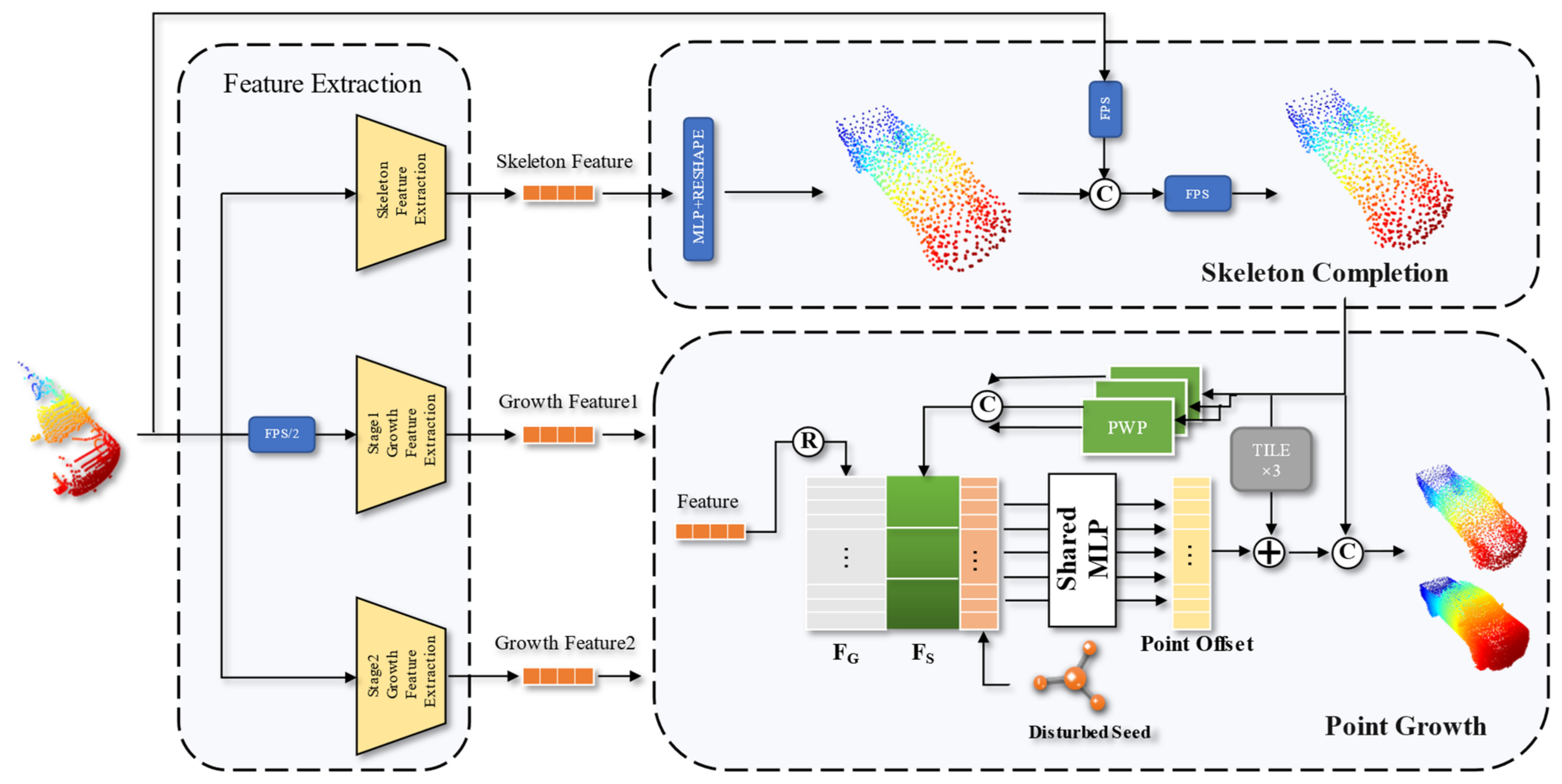
3.1. Overview
3.2. Composite Encoder Feature Extraction Module
3.3. Skeleton Point Cloud Generation Module
3.4. Point Cloud Growth Module
3.5. Training Loss
4. Experiments
4.1. Dataset
4.2. Metrics
4.3. Implementation Details
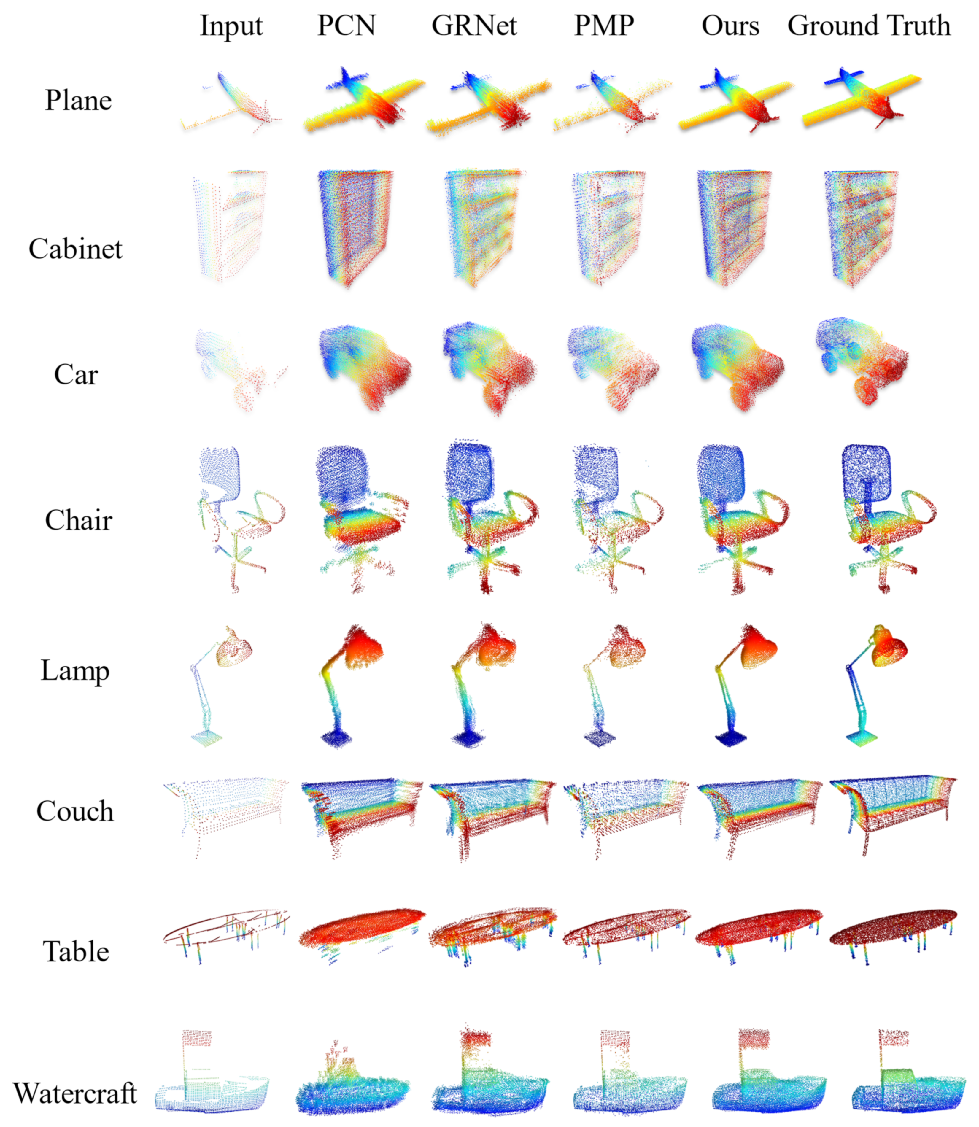
4.4. Completion Results on PCN
4.5. Completion Results on Completion3D
5. Model Analysis
5.1. Analysis of Composite Encoder Module
5.2. Analysis of Limited Sphere Neighborhood Radius
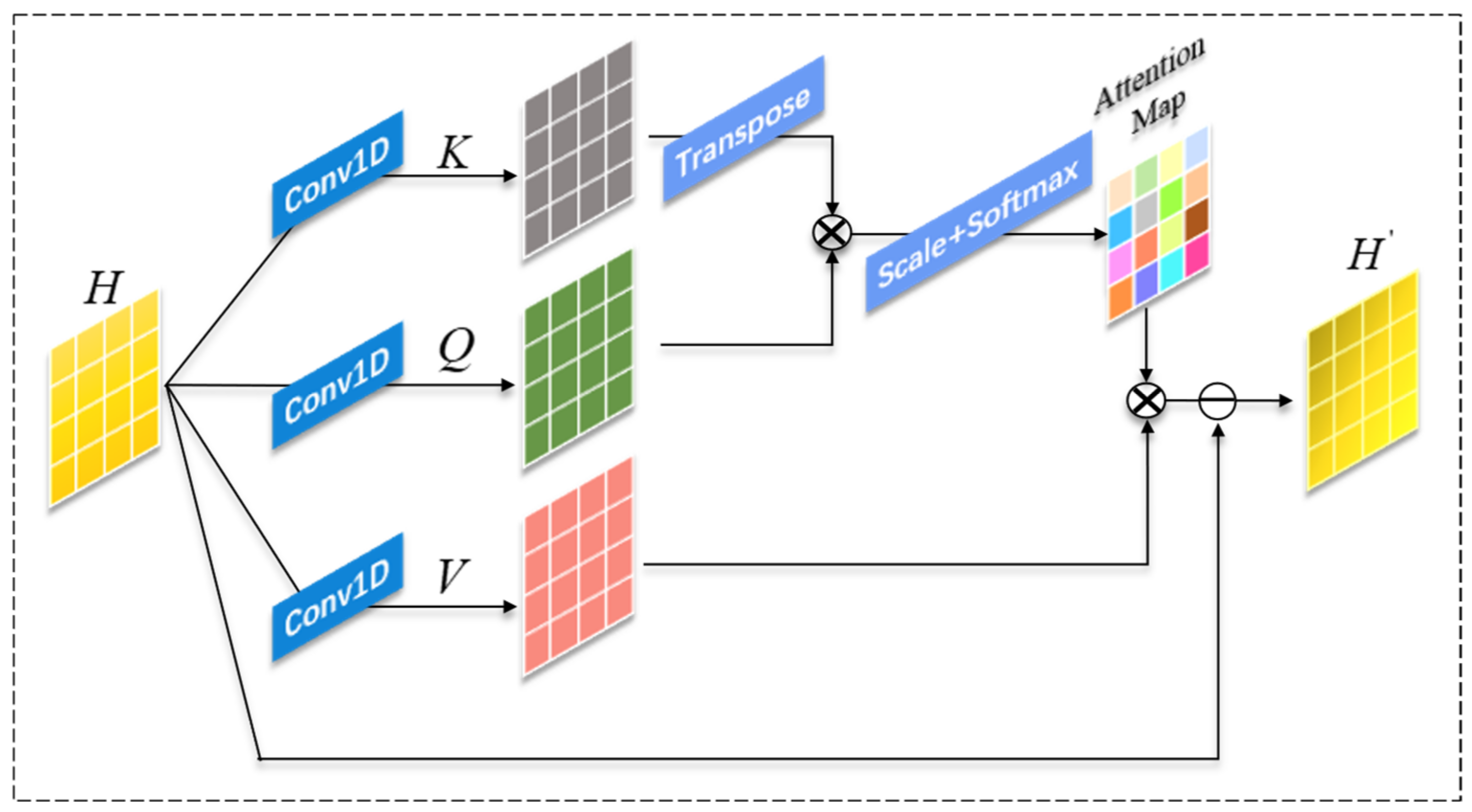
5.3. Analysis of Offset Transformer Structure
- (1)
- Remove Offset Transformer.
- (2)
- Replace Offset Transformer with channel-attention mechanism SE-Net [47].
- (3)
- Replace Offset Transformer with normal Transformer.
5.4. Analysis of PWP Decoding Structure
- (1)
- Splicing directly with the skeleton point coordinates and DFE features.
- (2)
- Splicing DFE features using folding in PCN.
- (3)
- No disturbance vector.
5.5. Ablation Experiments
6. Discussion
7. Conclusions
Author Contributions
Funding
Data Availability Statement
Conflicts of Interest
References
- Wang, Q.; Kim, M.-K. Applications of 3D point cloud data in the construction industry: A fifteen-year review from 2004 to 2018. Adv. Eng. Inform. 2019, 39, 306–319. [Google Scholar]
- Bisheng, Y.; Fuxun, L.; Ronggang, H. Progress, challenges and perspectives of 3D LiDAR point cloud processing. Acta Geod. Et Cartogr. Sin. 2017, 46, 1509. [Google Scholar]
- Horaud, R.; Hansard, M.; Evangelidis, G.; Ménier, C. An overview of depth cameras and range scanners based on time-of-flight technologies. Mach. Vis. Appl. 2016, 27, 1005–1020. [Google Scholar] [CrossRef]
- Teppati Losè, L.; Spreafico, A.; Chiabrando, F.; Giulio Tonolo, F. Apple LiDAR Sensor for 3D Surveying: Tests and Results in the Cultural Heritage Domain. Remote Sens. 2022, 14, 4157. [Google Scholar] [CrossRef]
- Van Oosterom, P.; Martinez-Rubi, O.; Ivanova, M.; Horhammer, M.; Geringer, D.; Ravada, S.; Tijssen, T.; Kodde, M.; Gonçalves, R. Massive point cloud data management: Design, implementation and execution of a point cloud benchmark. Comput. Graph. 2015, 49, 92–125. [Google Scholar] [CrossRef]
- Pang, G.; Qiu, R.; Huang, J.; You, S.; Neumann, U. Automatic 3D industrial point cloud modeling and recognition. In Proceedings of the 2015 14th IAPR International Conference on Machine Vision Applications (MVA), Tokyo, Japan, 18–22 May 2015. [Google Scholar]
- Pérez, L.; Rodríguez, Í.; Rodríguez, N.; Usamentiaga, R.; García, D.F. Robot guidance using machine vision techniques in industrial environments: A comparative review. Sensors 2016, 16, 335. [Google Scholar] [CrossRef]
- Kim, P.; Chen, J.; Cho, Y.K. SLAM-driven robotic mapping and registration of 3D point clouds. Autom. Constr. 2018, 89, 38–48. [Google Scholar] [CrossRef]
- Pi, D.; Liu, J.; Wang, Y. Review of computer-generated hologram algorithms for color dynamic holographic three-dimensional display. Light Sci. Appl. 2022, 11, 1–17. [Google Scholar] [CrossRef]
- Iglesias, L.; De Santos-Berbel, C.; Pascual, V.; Castro, M. Using Small Unmanned Aerial Vehicle in 3D Modeling of Highways with Tree-Covered Roadsides to Estimate Sight Distance. Remote Sens. 2019, 11, 2625. [Google Scholar] [CrossRef]
- Qi, C.R.; Su, H.; Mo, K.; Guibas, L.J. Pointnet: Deep learning on point sets for 3d classification and segmentation. In Proceedings of the IEEE Conference on Computer Vision and Pattern Recognition, Honolulu, HI, USA, 21–26 July 2017. [Google Scholar]
- Uy, M.A.; Pham, Q.-H.; Hua, B.-S.; Nguyen, T.; Yeung, S.-K. Revisiting point cloud classification: A new benchmark dataset and classification model on real-world data. In Proceedings of the IEEE/CVF International Conference on Computer Vision, Seoul, Korea, 27 October–2 November 2019. [Google Scholar]
- Li, J.; Chen, B.; Lee, G.H. So-net: Self-organizing network for point cloud analysis. In Proceedings of the IEEE Conference on Computer Vision and Pattern Recognition, Salt Lake City, UT, USA, 18–23 June 2018. [Google Scholar]
- Zhu, K.; He, X.; Gao, Y.; Hao, R.; Wei, Z.; Long, B.; Mu, Z.; Wang, J. Invalid point removal method based on error energy function in fringe projection profilometry. Results Phys. 2022, 41, 105904. [Google Scholar] [CrossRef]
- Song, W.; Li, D.; Sun, S.; Zhang, L.; Xin, Y.; Sung, Y.; Choi, R. 2D&3DHNet for 3D Object Classification in LiDAR Point Cloud. Remote Sens. 2022, 14, 3146. [Google Scholar]
- Singer, N.; Asari, V.K. View-Agnostic Point Cloud Generation for Occlusion Reduction in Aerial Lidar. Remote Sens. 2022, 14, 2955. [Google Scholar] [CrossRef]
- Liu, G.; Wei, S.; Zhong, S.; Huang, S.; Zhong, R. Reconstruction of Indoor Navigation Elements for Point Cloud of Buildings with Occlusions and Openings by Wall Segment Restoration from Indoor Context Labeling. Remote Sens. 2022, 14, 4275. [Google Scholar] [CrossRef]
- Qi, C.R.; Yi, L.; Su, H.; Guibas, L.J. Pointnet++: Deep hierarchical feature learning on point sets in a metric space. Adv. Neural Inf. Process. Syst. 2017, 30, 5105–5114. [Google Scholar]
- Ni, P.; Zhang, W.; Zhu, X.; Cao, Q. Pointnet++ grasping: Learning an end-to-end spatial grasp generation algorithm from sparse point clouds. In Proceedings of the 2020 IEEE International Conference on Robotics and Automation (ICRA), Paris, France, 31 May–31 August 2020. [Google Scholar]
- Chen, Y.; Liu, G.; Xu, Y.; Pan, P.; Xing, Y. PointNet++ network architecture with individual point level and global features on centroid for ALS point cloud classification. Remote Sens. 2021, 13, 472. [Google Scholar] [CrossRef]
- Yang, Y.; Feng, C.; Shen, Y.; Tian, D. Foldingnet: Point cloud auto-encoder via deep grid deformation. In Proceedings of the IEEE Conference on Computer Vision and Pattern Recognition, Salt Lake City, UT, USA, 18–23 June 2018. [Google Scholar]
- Yuan, W.; Khot, T.; Held, D.; Mertz, C.; Hebert, M. Pcn: Point completion network. In Proceedings of the 2018 International Conference on 3D Vision (3DV), Verona, Italy, 5–8 September 2018. [Google Scholar]
- Tchapmi, L.P.; Kosaraju, V.; Rezatofighi, H.; Reid, I.; Savarese, S. Topnet: Structural point cloud decoder. In Proceedings of the IEEE/CVF Conference on Computer Vision and Pattern Recognition, Long Beach, CA, USA, 15–20 June 2019. [Google Scholar]
- Xie, H.; Yao, H.; Zhou, S.; Mao, J.; Zhang, S.; Sun, W. Grnet: Gridding residual network for dense point cloud completion. In Proceedings of the European Conference on Computer Vision, Glasgow, UK, 23–28 August 2020; Springer: Berlin/Heidelberg, Germany, 2020. [Google Scholar]
- Zhang, J.; Shao, J.; Chen, J.; Yang, D.; Liang, B.; Liang, R. PFNet: An unsupervised deep network for polarization image fusion. Opt. Lett. 2020, 45, 1507–1510. [Google Scholar]
- Wen, X.; Xiang, P.; Han, Z.; Cao, Y.-P.; Wan, P.; Zheng, W.; Liu, Y.-S. Pmp-net: Point cloud completion by learning multi-step point moving paths. In Proceedings of the IEEE/CVF Conference on Computer Vision and Pattern Recognition, Nashville, TN, USA, 20–25 June 2021. [Google Scholar]
- Carr, J.C.; Beatson, R.K.; Cherrie, J.B.; Mitchell, T.J.; Fright, W.R.; McCallum, B.C.; Evans, T.R. Reconstruction and representation of 3D objects with radial basis functions. In Proceedings of the 28th Annual Conference on Computer Graphics and Interactive Techniques, Los Angeles, CA, USA, 12–17 August 2001. [Google Scholar]
- Li, Y.; Dai, A.; Guibas, L.; Nießner, M. Database-assisted object retrieval for real-time 3d reconstruction. In Computer Graphics Forum; Wiley Online Library: Hoboken, NJ, USA, 2015. [Google Scholar]
- Pauly, M.; Mitra, N.J.; Wallner, J.; Pottmann, H.; Guibas, L.J. Discovering structural regularity in 3D geometry. In ACM SIGGRAPH 2008 Papers; Association for Computing Machinery: New York, NY, USA, 2008; pp. 1–11. [Google Scholar]
- Gupta, S.; Arbeláez, P.; Girshick, R.; Malik, J. Aligning 3D models to RGB-D images of cluttered scenes. In Proceedings of the IEEE Conference on Computer Vision and Pattern Recognition, Boston, MA, USA, 7–12 June 2015. [Google Scholar]
- Su, H.; Maji, S.; Kalogerakis, E. Learned-Miller Multi-view convolutional neural networks for 3d shape recognition. In Proceedings of the IEEE International Conference on Computer Vision, Santiago, Chile, 7–13 December 2015. [Google Scholar]
- Pang, G.; Neumann, U. 3D point cloud object detection with multi-view convolutional neural network. In Proceedings of the 23rd International Conference on Pattern Recognition (ICPR), Cancun, Mexico, 4–8 December 2016. [Google Scholar]
- Yang, B.; Wen, H.; Wang, S.; Clark, R.; Markham, A.; Trigoni, N. 3D object reconstruction from a single depth view with adversarial learning. In Proceedings of the IEEE International Conference on Computer Vision Workshops, Venice, Italy, 22–29 October 2017. [Google Scholar]
- Dai, A.; Qi, C.R.; Nießner, M. Shape completion using 3D-encoder-predictor cnns and shape synthesis. In Proceedings of the IEEE Conference on Computer Vision and Pattern Recognition, Honolulu, HI, USA, 21–26 July 2017. [Google Scholar]
- Wang, W.; Huang, Q.; You, S.; Yang, C.; Neumann, U. Shape inpainting using 3d generative adversarial network and recurrent convolutional networks. In Proceedings of the IEEE International Conference on Computer Vision, Venice, Italy, 22–29 October 2017. [Google Scholar]
- Wang, Y.; Sun, Y.; Liu, Z.; Sarma, S.E.; Bronstein, M.M.; Solomon, J.M. Dynamic graph cnn for learning on point clouds. Acm Trans. Graph. 2019, 38, 1–12. [Google Scholar] [CrossRef]
- Li, Y.; Bu, R.; Sun, M.; Wu, W.; Di, X.; Chen, B. Pointcnn: Convolution on x-transformed points. Adv. Neural Inf. Process. Syst. 2018, 31. [Google Scholar]
- Liu, M.; Sheng, L.; Yang, S.; Shao, J.; Hu, S.-M. Morphing and sampling network for dense point cloud completion. In Proceedings of the AAAI Conference on Artificial Intelligence, New York, NY, USA, 7–12 February 2020. [Google Scholar]
- Wang, Y.; Tan, D.J.; Navab, N.; Tombari, F. Softpoolnet: Shape descriptor for point cloud completion and classification. In Proceedings of the European Conference on Computer Vision, Glasgow, UK, 23–28 August 2020; Springer: Berlin/Heidelberg, Germany, 2020. [Google Scholar]
- Vaswani, A.; Shazeer, N.; Parmar, N.; Uszkoreit, J.; Jones, L.; Gomez, A.N.; Kaiser, Ł.; Polosukhin, I. Attention is all you need. Adv. Neural Inf. Process. Syst. 2017, 30, 6000–6010. [Google Scholar]
- Guo, M.-H.; Cai, J.-X.; Liu, Z.-N.; Mu, T.-J.; Martin, R.R.; Hu, S.-M. Pct: Point cloud transformer. Comput. Vis. Media 2021, 7, 187–199. [Google Scholar] [CrossRef]
- Zhao, H.; Jiang, L.; Jia, J.; Torr, P.H.; Koltun, V. Point transformer. In Proceedings of the IEEE/CVF International Conference on Computer Vision, Montreal, QC, Canada, 11–17 October 2021. [Google Scholar]
- Tatarchenko, M.; Richter, S.R.; Ranftl, R.; Li, Z.; Koltun, V.; Brox, T. What do single-view 3d reconstruction networks learn? In Proceedings of the IEEE/CVF Conference on Computer Vision and Pattern Recognition, Long Beach, CA, USA, 15–20 June 2019.
- Groueix, T.; Fisher, M.; Kim, V.G.; Russell, B.C.; Aubry, M. A papier-mâché approach to learning 3d surface generation. In Proceedings of the IEEE Conference on Computer Vision and Pattern Recognition, Salt Lake City, UT, USA, 18–23 June 2018. [Google Scholar]
- Zhang, J.; Chen, W.; Wang, Y.; Vasudevan, R.; Johnson-Roberson, M. Point set voting for partial point cloud analysis. IEEE Robot. Autom. Lett. 2021, 6, 596–603. [Google Scholar] [CrossRef]
- Wen, X.; Li, T.; Han, Z.; Liu, Y.-S. Point cloud completion by skip-attention network with hierarchical folding. In Proceedings of the IEEE/CVF Conference on Computer Vision and Pattern Recognition, Seattle, WA, USA, 13–19 June 2020. [Google Scholar]
- Hu, J.; Shen, L.; Sun, G. Squeeze-and-excitation networks. In Proceedings of the IEEE Conference on Computer Vision and Pattern Recognition, Salt Lake City, UT, USA, 18–23 June 2018. [Google Scholar]


| Methods | Average | Plane | Cabinet | Car | Chair | Lamp | Couch | Table | Watercraft |
|---|---|---|---|---|---|---|---|---|---|
| 3D-EPN [34] | 20.15 | 13.16 | 21.8 | 20.31 | 18.81 | 25.75 | 21.09 | 21.72 | 18.54 |
| POINTNET++ [18] | 14 | 10.3 | 14.74 | 12.19 | 15.78 | 17.62 | 16.18 | 11.68 | 13.52 |
| FOLDINGNET [21] | 14.31 | 9.49 | 15.8 | 12.61 | 15.55 | 16.41 | 15.97 | 13.65 | 14.99 |
| TOPNET [23] | 12.15 | 7.61 | 13.31 | 10.9 | 13.82 | 14.44 | 14.78 | 11.22 | 11.12 |
| ATLASNET [44] | 10.85 | 6.37 | 11.94 | 10.1 | 12.06 | 12.37 | 12.99 | 10.33 | 10.61 |
| PCN [22] | 9.64 | 5.5 | 22.7 | 10.63 | 10.99 | 11 | 11.34 | 11.68 | 8.59 |
| SOFTPOOLNET [39] | 9.205 | 6.93 | 10.91 | 9.78 | 9.56 | 8.59 | 11.22 | 8.51 | 8.14 |
| MSN [38] | 9.97 | 5.6 | 11.96 | 10.78 | 10.62 | 10.71 | 11.9 | 8.7 | 9.49 |
| GRNET [24] | 8.83 | 6.45 | 10.37 | 9.45 | 9.41 | 7.96 | 10.51 | 8.44 | 8.04 |
| PMP [26] | 8.73 | 5.65 | 11.24 | 9.64 | 9.51 | 6.95 | 10.83 | 8.72 | 7.25 |
| OURS | 8.59 | 4.85 | 10.44 | 8.32 | 9.95 | 7.56 | 11.15 | 8.31 | 8.18 |
| Methods | Average | Plane | Cabinet | Car | Chair | Lamp | Couch | Table | Watercraft |
|---|---|---|---|---|---|---|---|---|---|
| ATLASNET [44] | 0.616 | 0.845 | 0.552 | 0.630 | 0.552 | 0.565 | 0.500 | 0.660 | 0.624 |
| PCN [22] | 0.695 | 0.881 | 0.651 | 0.725 | 0.625 | 0.638 | 0.581 | 0.765 | 0.697 |
| FOLDINGNET [21] | 0.322 | 0.642 | 0.237 | 0.382 | 0.236 | 0.219 | 0.197 | 0.361 | 0.299 |
| TOPNET [23] | 0.503 | 0.771 | 0.404 | 0.544 | 0.413 | 0.408 | 0.350 | 0.572 | 0.560 |
| MSN [38] | 0.705 | 0.885 | 0.644 | 0.665 | 0.657 | 0.699 | 0.604 | 0.782 | 0.708 |
| GRNET [24] | 0.708 | 0.843 | 0.618 | 0.682 | 0.673 | 0.761 | 0.605 | 0.751 | 0.750 |
| OURS | 0.729 | 0.913 | 0.650 | 0.749 | 0.680 | 0.749 | 0.612 | 0.788 | 0.754 |
| Methods | Average | Plane | Cabinet | Car | Chair | Lamp | Couch | Table | Watercraft |
|---|---|---|---|---|---|---|---|---|---|
| FOLDINGNET [21] | 19.07 | 12.83 | 23.01 | 14.88 | 25.69 | 21.79 | 21.31 | 20.71 | 11.51 |
| PCN [22] | 18.22 | 9.79 | 22.7 | 12.43 | 25.14 | 22.72 | 20.26 | 20.27 | 11.73 |
| POINTSETV [45] | 18.18 | 6.88 | 21.18 | 15.78 | 22.54 | 18.78 | 28.39 | 19.96 | 11.16 |
| ATLASNET [44] | 17.77 | 10.36 | 23.4 | 13.4 | 24.16 | 20.24 | 20.82 | 17.52 | 11.62 |
| SOFTPOOLNET [39] | 16.15 | 5.81 | 24.53 | 11.35 | 23.63 | 18.54 | 20.34 | 16.89 | 7.14 |
| TOPNET [23] | 14.25 | 7.32 | 18.77 | 12.88 | 19.82 | 14.6 | 16.29 | 14.89 | 8.82 |
| SA-NET [46] | 11.22 | 5.27 | 14.45 | 7.78 | 13.67 | 13.53 | 14.22 | 11.75 | 8.84 |
| GRNET [24] PMP [26] | 10.64 9.23 | 6.13 3.99 | 16.9 14.7 | 8.27 8.55 | 12.23 10.21 | 10.22 9.27 | 14.93 12.43 | 10.08 8.51 | 5.86 5.77 |
| OURS | 8.87 | 2.92 | 13.53 | 6.01 | 11.05 | 10.76 | 9.15 | 11.87 | 5.71 |
| Evaluate | Avg. | Airplane | Car | Couch | Watercraft |
|---|---|---|---|---|---|
| PointNet | 9.125 | 5.72 | 9.32 | 12.15 | 9.23 |
| PointNet++ | 8.53 | 5.50 | 8.97 | 11.43 | 8.22 |
| DGCNN | 8.57 | 5.53 | 8.78 | 11.46 | 8.51 |
| CE | 8.13 | 4.85 | 8.32 | 11.15 | 8.18 |
| Radius | Avg. | Airplane | Car | Couch | Watercraft |
|---|---|---|---|---|---|
| [0.5, 0.25] | 8.46 | 5.05 | 8.9 | 11.51 | 8.39 |
| [0.4, 0.2] | 8.26 | 5.07 | 8.7 | 11.02 | 8.27 |
| [0.2, 0.1] | 8.13 | 4.85 | 8.32 | 11.15 | 8.18 |
| [0.1, 0.05] | 8.29 | 5.11 | 8.27 | 11.32 | 8.46 |
| [0.02, 0.01] | 8.61 | 5.32 | 8.86 | 11.63 | 8.59 |
| Evaluate | Avg. | Airplane | Car | Couch | Watercraft |
|---|---|---|---|---|---|
| w/o Attention | 8.35 | 4.94 | 8.55 | 11.53 | 8.38 |
| SE | 8.26 | 5.01 | 8.33 | 11.46 | 8.22 |
| Normal Transformer | 8.16 | 4.92 | 8.37 | 11.32 | 8.06 |
| Offset Transformer | 8.13 | 4.85 | 8.32 | 11.15 | 8.18 |
| Evaluate | Avg. | Airplane | Car | Couch | Watercraft |
|---|---|---|---|---|---|
| Point cloud coordinates | 9.26 | 5.76 | 10.65 | 11.88 | 8.74 |
| PCN-FOLDING | 8.82 | 5.25 | 10.37 | 11.24 | 8.42 |
| w/o disturb | 8.21 | 4.96 | 8.43 | 11.25 | 8.19 |
| PWP | 8.13 | 4.85 | 8.32 | 11.15 | 8.18 |
| MAPGNet w/o Offset Transformer | MAPGNet w/o CE + POINTNET++ | MAPGNet w/o PWP + FOLDING | MAPGNet | |
|---|---|---|---|---|
| Avg. | 8.35 | 8.53 | 8.82 | 8.13 |
| Enhance Percent | 2.71% | 4.82% | 8.49% | / |
Publisher’s Note: MDPI stays neutral with regard to jurisdictional claims in published maps and institutional affiliations. |
© 2022 by the authors. Licensee MDPI, Basel, Switzerland. This article is an open access article distributed under the terms and conditions of the Creative Commons Attribution (CC BY) license (https://creativecommons.org/licenses/by/4.0/).
Share and Cite
Hao, R.; Wei, Z.; He, X.; Zhu, K.; Wang, J.; He, J.; Zhang, L. Multistage Adaptive Point-Growth Network for Dense Point Cloud Completion. Remote Sens. 2022, 14, 5214. https://doi.org/10.3390/rs14205214
Hao R, Wei Z, He X, Zhu K, Wang J, He J, Zhang L. Multistage Adaptive Point-Growth Network for Dense Point Cloud Completion. Remote Sensing. 2022; 14(20):5214. https://doi.org/10.3390/rs14205214
Chicago/Turabian StyleHao, Ruidong, Zhonghui Wei, Xu He, Kaifeng Zhu, Jun Wang, Jiawei He, and Lei Zhang. 2022. "Multistage Adaptive Point-Growth Network for Dense Point Cloud Completion" Remote Sensing 14, no. 20: 5214. https://doi.org/10.3390/rs14205214
APA StyleHao, R., Wei, Z., He, X., Zhu, K., Wang, J., He, J., & Zhang, L. (2022). Multistage Adaptive Point-Growth Network for Dense Point Cloud Completion. Remote Sensing, 14(20), 5214. https://doi.org/10.3390/rs14205214