
Predicting Habitat Properties Using Remote Sensing Data: Soil pH and Moisture, and Ground Vegetation Cover


Abstract
1. Introduction
2. Materials and Methods
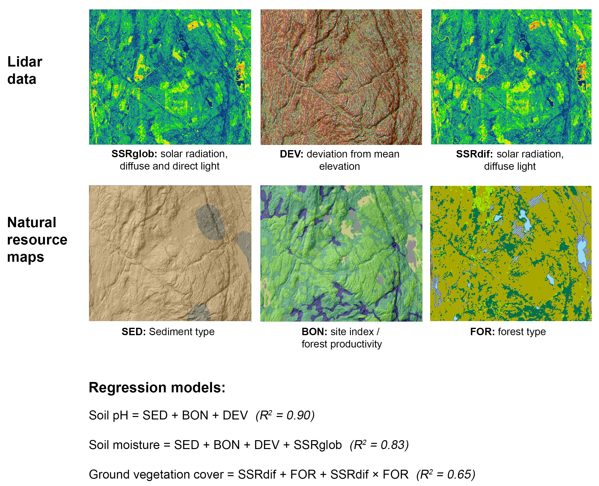
2.1. Study Area
2.2. Field Data Collection and Processing
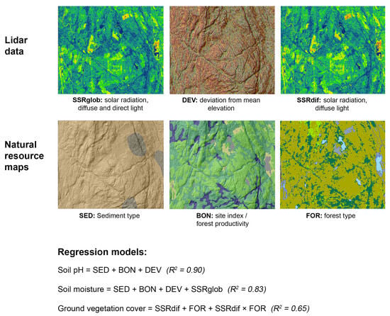
2.3. Generating Predictor Variables from Remote Sensing Data
2.4. Additional Information Included
2.5. Statistical Analysis
3. Results
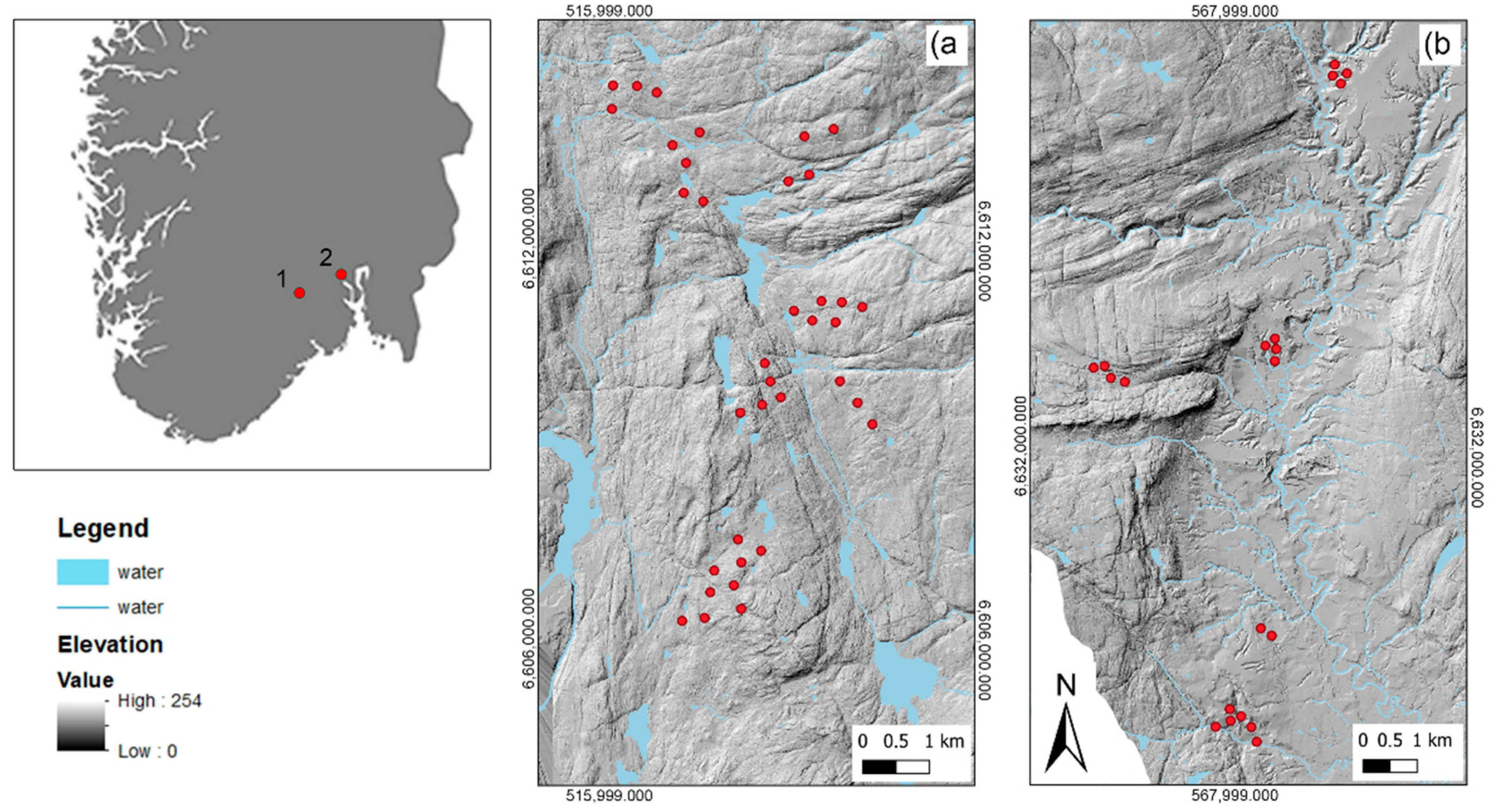
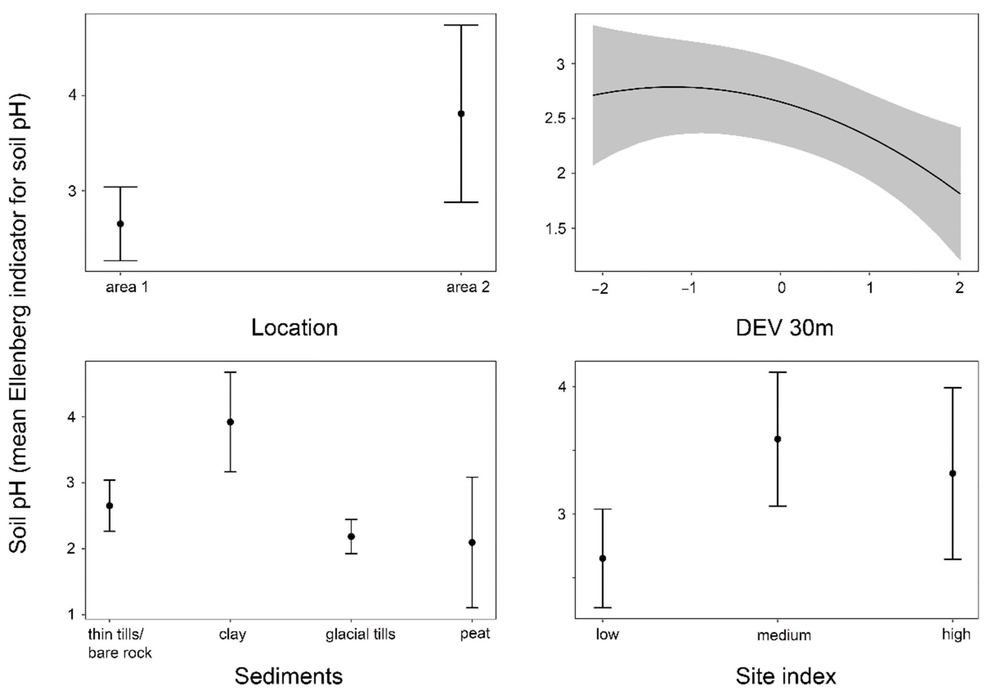
3.1. Soil pH
- Soil pH = a + b1(SED) + b2(LOC) + b3(BON) + b4(DEV30M)2 + e
- Soil pH = a + b1(SED) + b2(LOC) + b3(BON) + b4(DEV30M)2 + b5(SWI1m) +e
- Soil pH = a + b1(SED) + b2(LOC) + b3(BON) + b4(DEV30M)2 + b5(SLOP) + e
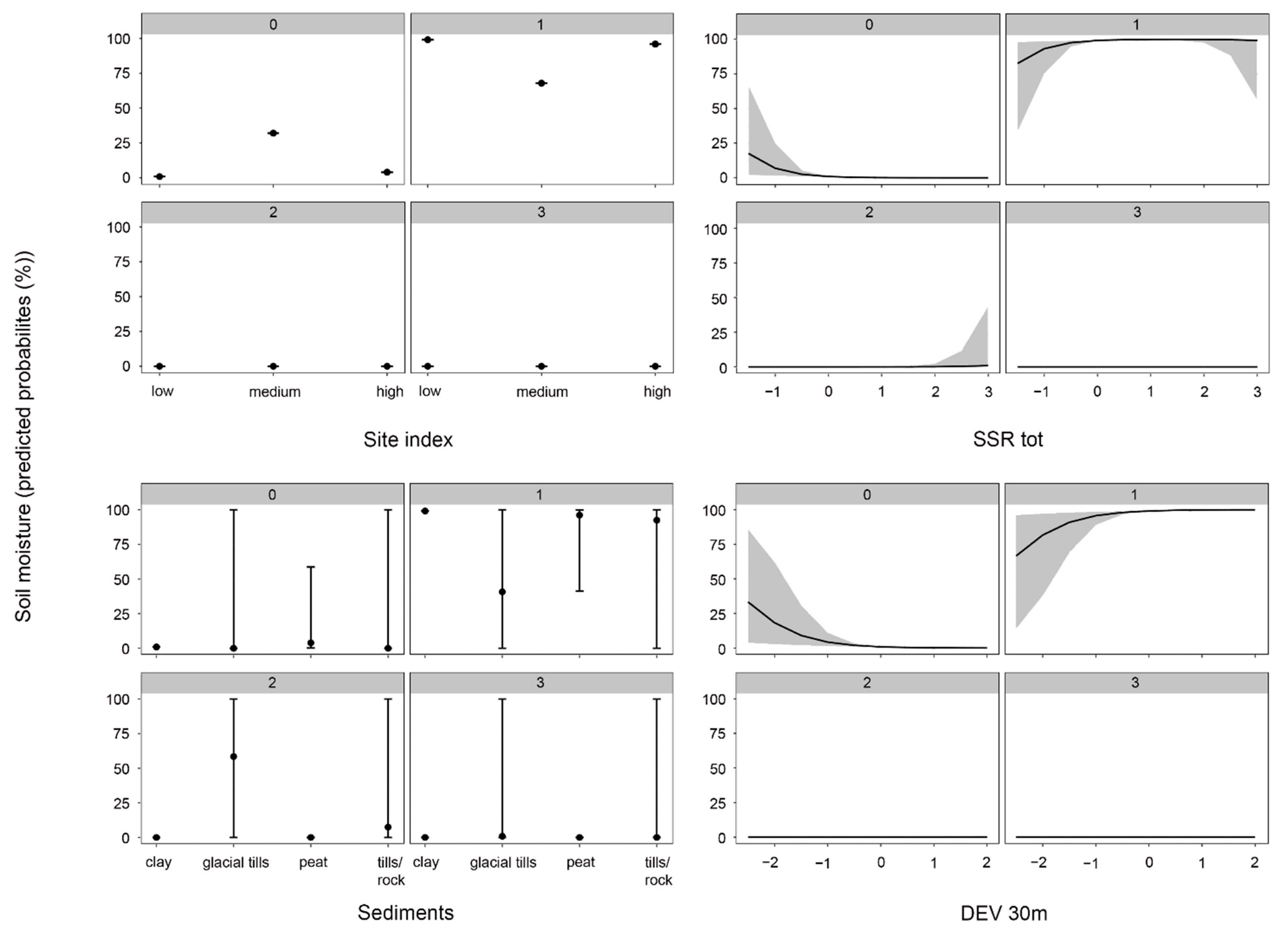
3.2. Soil Moisture
- Soil moist. = a + b1(BON) + b2(SED) + b3(SSRglob) + b4(DEV30M) + e
- Soil moist. = a + b1(BON) + b2(LOC) + b3(SSRglob) + b4(DEV30M) + e
- Soil moist. = a + b1(BON) + b2(SED) + b3(SSRglob) + b4(DEV30M) + b5(DEP)+ e
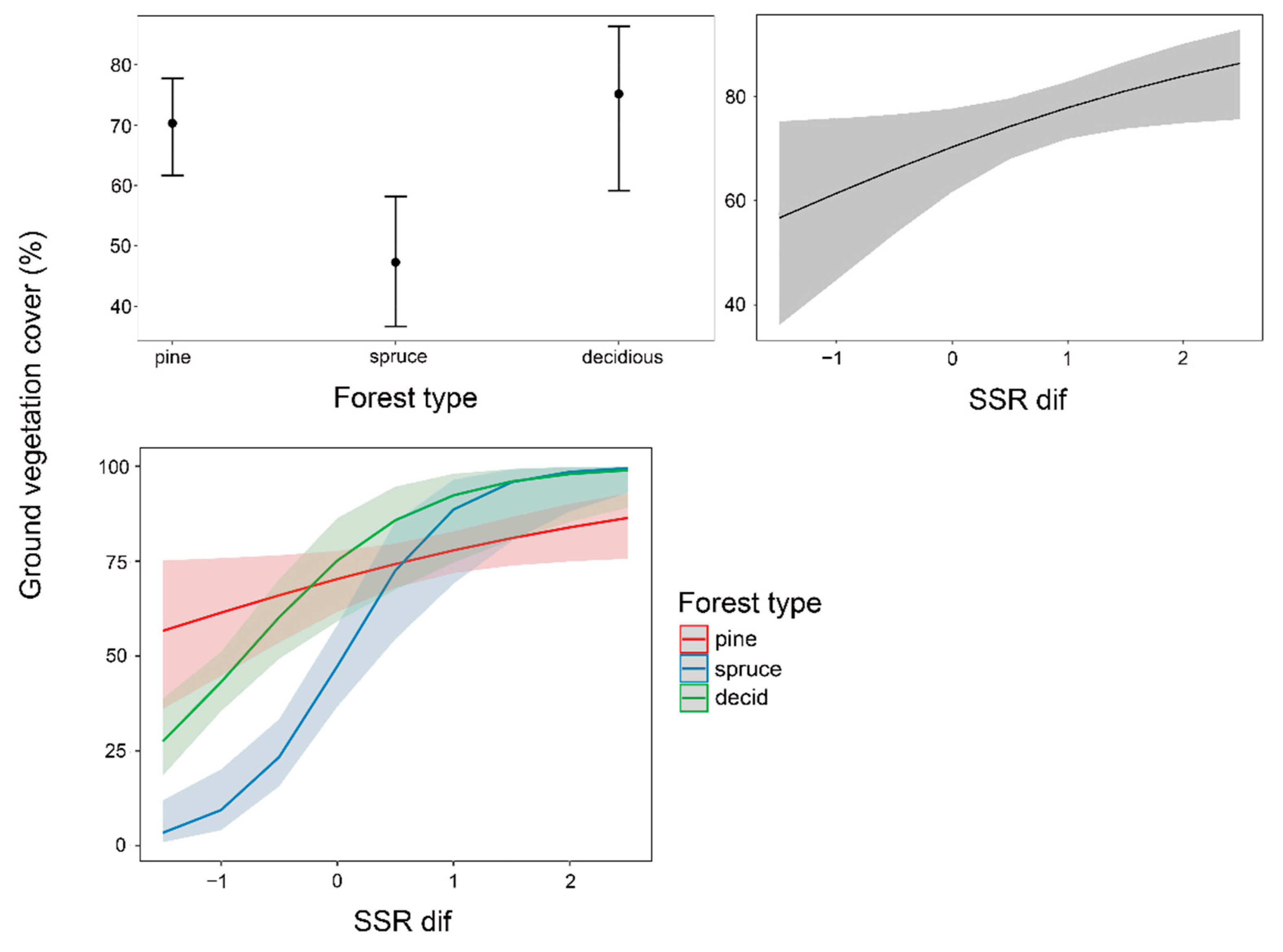
3.3. Ground Vegetation Cover
- G. veg. cov. = a + b1(FOR) + b2(SSRdif) + b3(FOR) × (SSRdif) + e
- G. veg. cov. = a + b1(FOR) + b2(SSRdif) + b3(FOR) × (SSRdif) + b4(DEV30M) + e
- G. veg. cov. = a + b1(FOR) + b2(SSRdif) + b3(FOR) × (SSRdif) + b4(SLOP) + e
4. Discussion
5. Conclusions
Supplementary Materials
Author Contributions
Data Availability Statement
Acknowledgments
Conflicts of Interest
References
- Chuvieco, E. Fundamentals of Satellite Remote Sensing: An Environmental Approach, 3rd ed.; CRC Press: New York, NY, USA, 2020. [Google Scholar]
- Randin, C.F.; Ashcroft, M.B.; Bolliger, J.; Cavender-Bares, J.; Coops, N.C.; Dullinger, S.; Dirnböck, T.; Eckert, S.; Ellis, E.; Fernández, N.; et al. Monitoring biodiversity in the Anthropocene using remote sensing in species distribution models. Remote Sens. Environ. 2020, 239, 111626. [Google Scholar] [CrossRef]
- de Araujo Barbosa, C.C.; Atkinson, P.M.; Dearing, J.A. Remote sensing of ecosystem services: A systematic review. Ecol. Indic. 2015, 52, 430–443. [Google Scholar] [CrossRef]
- Poursanidis, D.; Traganos, D.; Reinartz, P.; Chrysoulakis, N. On the use of Sentinel-2 for coastal habitat mapping and satellite-derived bathymetry estimation using downscaled coastal aerosol band. Int. J. Appl. Earth Obs. Geoinf. 2019, 80, 58–70. [Google Scholar] [CrossRef]
- Ackers, S.H.; Davis, R.J.; Olsen, K.A.; Dugger, K.M. The evolution of mapping habitat for northern spotted owls (Strix occidentalis caurina): A comparison of photo-interpreted, Landsat-based, and lidar-based habitat maps. Remote Sens. Environ. 2015, 156, 361–373. [Google Scholar] [CrossRef]
- Wenger, S.J.; Olden, J.D. Assessing transferability of ecological models: An underappreciated aspect of statistical validation. Methods Ecol. Evol. 2012, 3, 260–267. [Google Scholar] [CrossRef]
- Li, X.; Chang, S.X.; Liu, J.; Zheng, Z.; Wang, X. Topography-soil relationships in a hilly evergreen broadleaf forest in subtropical China. J. Soils Sediments 2016, 17, 1101–1115. [Google Scholar] [CrossRef]
- Aagren, A.M.; Larson, J.; Paul, S.S.; Laudon, H.; Lidberg, W. Use of multiple LIDAR-derived digital terrain indices and machine learning for high-resolution national-scale soil moisture mapping of the Swedish forest landscape. Geoderma 2021, 404, 115280. [Google Scholar] [CrossRef]
- Oltean, G.S.; Comeau, P.G.; White, B. Linking the depth-to-water topographic index to soil moisture on boreal forest sites in Alberta. For. Sci. 2016, 62, 154–165. [Google Scholar] [CrossRef]
- Bode, C.A.; Limm, M.P.; Power, M.E.; Finlay, J.C. Subcanopy Solar Radiation model: Predicting solar radiation across a heavily vegetated landscape using LiDAR and GIS solar radiation models. Remote Sens. Environ. 2014, 154, 387–397. [Google Scholar] [CrossRef]
- Zellweger, F.; Baltensweiler, A.; Schleppi, P.; Huber, M.; Küchler, M.; Ginzler, C.; Jonas, T. Estimating below-canopy light regimes using airborne laser scanning: An application to plant community analysis. Ecol. Evol. 2019, 9, 9149–9159. [Google Scholar] [CrossRef]
- Chew, C.; Shah, R.; Zuffada, C.; Hajj, G.; Masters, D.; Mannucci, A.J. Demonstrating soil moisture remote sensing with observations from the UK TechDemoSat-1 satellite mission. Geophys. Res. Lett. 2016, 43, 3317–3324. [Google Scholar] [CrossRef]
- Baines, D.; Moss, R.; Dugan, D. Capercaillie breeding success in relation to forest habitat and predator abundance. J. Appl. Ecol. 2004, 41, 59–71. [Google Scholar] [CrossRef]
- Telagathoti, A.; Probst, M.; Peintner, U. Habitat, Snow-Cover and Soil pH, Affect the Distribution and Diversity of Mortierellaceae Species and Their Associations to Bacteria. Front. Microbiol. 2021, 12, 669784. [Google Scholar] [CrossRef] [PubMed]
- Wang, J.-T.; Zheng, Y.-M.; Hu, H.-W.; Zhang, L.-M.; Li, J.; He, J.-Z. Soil pH determines the alpha diversity but not beta diversity of soil fungal community along altitude in a typical Tibetan forest ecosystem. J. Soils Sediments 2015, 15, 1224–1232. [Google Scholar] [CrossRef]
- Erlandson, S.; Savage, J.; Cavender-Bares, J.; Peay, K. Soil moisture and chemistry influence diversity of ectomycorrhizal fungal communities associating with willow along an hydrologic gradient. FEMS Microbiol. Ecol. 2016, 92, 1–9. [Google Scholar] [CrossRef] [PubMed]
- Nilsson, M.-C.; Wardle, D.A. Understory Vegetation as a Forest Ecosystem Driver: Evidence from the Northern Swedish Boreal Forest. Front. Ecol. Environ. 2005, 3, 421–428. [Google Scholar] [CrossRef]
- Liu, L.; Gudmundsson, L.; Hauser, M.; Qin, D.; Li, S.; Seneviratne, S.I. Soil moisture dominates dryness stress on ecosystem production globally. Nat. Commun. 2020, 11, 4892. [Google Scholar] [CrossRef]
- Emmett, B.A.; Cooper, D.; Smart, S.; Jackson, B.; Thomas, A.; Cosby, B.; Evans, C.; Glanville, H.; McDonald, J.E.; Malham, S.K.; et al. Spatial patterns and environmental constraints on ecosystem services at a catchment scale. Sci. Total Environ. 2016, 572, 1586–1600. [Google Scholar] [CrossRef]
- Weil, R.R.; Brady, N.C.; Weil, R.R. The Nature and Properties of Soils, 5th ed.; Pearson: Harlow, UK, 2017. [Google Scholar]
- Seibert, J.; Stendahl, J.; Sørensen, R. Topographical influences on soil properties in boreal forests. Geoderma 2007, 141, 139–148. [Google Scholar] [CrossRef]
- Barbier, S.; Gosselin, F.; Balandier, P. Influence of tree species on understory vegetation diversity and mechanisms involved—A critical review for temperate and boreal forests. For. Ecol. Manag. 2008, 254, 1–15. [Google Scholar] [CrossRef]
- Augusto, L.; De Schrijver, A.; Vesterdal, L.; Smolander, A.; Prescott, C.; Ranger, J. Influences of evergreen gymnosperm and deciduous angiosperm tree species on the functioning of temperate and boreal forests: Spermatophytes and forest functioning. Biol. Rev. Camb. Philos. Soc. 2015, 90, 444–466. [Google Scholar] [CrossRef] [PubMed]
- Amaro, A.; Reed, D.; Soares, P. Modelling Forest Systems; CABI: Yuen Long, Hong Kong, 2003. [Google Scholar]
- Farrelly, N.; Ní Dhubháin, Á.; Nieuwenhuis, M. Site index of Sitka spruce (Picea sitchensis) in relation to different measures of site quality in Ireland. Rev. Can. De Rech. For. 2011, 41, 265–278. [Google Scholar] [CrossRef]
- Neina, D. The Role of Soil pH in Plant Nutrition and Soil Remediation. Appl. Environ. Soil Sci. 2019, 2019, 5794869. [Google Scholar] [CrossRef]
- Western, A.W.; Grayson, R.B.; Blöschl, G. SCALING OF SOIL MOISTURE: A Hydrologic Perspective. Annu. Rev. Earth Planet. Sci. 2002, 30, 149–180. [Google Scholar] [CrossRef]
- Oke, T.R. Boundary Layer Climates, 2nd ed.; Routledge: London, UK, 1987; p. 464. [Google Scholar]
- Lid, J.; Lid, D.T.; Elven, R.; Alm, T. Norsk Flora, 7th ed.; Samlaget: Oslo, Norway, 2005. [Google Scholar]
- Hart, S.A.; Chen, H.Y.H. Understory Vegetation Dynamics of North American Boreal Forests. Crit. Rev. Plant Sci. 2006, 25, 381–397. [Google Scholar] [CrossRef]
- Asbjornsen, H.; Goldsmith, G.R.; Alvarado-Barrientos, M.S.; Rebel, K.T.; Osch, F.v.; Rietkerk, M.G.; Chen, J.; Gotsch, S.; Tobon, C.; Geissert, D.R.; et al. Ecohydrological advances and applications in plant-water relations research: A review. Plant Ecol. 2011, 4, 3. [Google Scholar] [CrossRef]
- Burke, I.C.; Lauenroth, W.K.; Vinton, M.A.; Hook, P.B.; Kelly, R.H.; Epstein, H.E.; Aguiar, M.R.; Robles, M.D.; Aguilera, M.O.; Murphy, K.L.; et al. Plant-soil interactions in temperate grasslands. Biogeochemistry 1998, 42, 121–143. [Google Scholar] [CrossRef]
- Bochet, E.; García-Fayos, P. Factors Controlling Vegetation Establishment and Water Erosion on Motorway Slopes in Valencia, Spain. Restor. Ecol. 2004, 12, 166–174. [Google Scholar] [CrossRef]
- Natur i Norge. Available online: https://artsdatabanken.no/NiN (accessed on 14 January 2022).
- Halvorsen, R.; Skarpaas, O.; Bryn, A.; Bratli, H.; Erikstad, L.; Simensen, T.; Lieungh, E.; Zarnetske, P. Towards a systematics of ecodiversity: The EcoSyst framework. Glob. Ecol. Biogeogr. 2020, 29, 1887–1906. [Google Scholar] [CrossRef]
- Ellenberg, H.; Leuschner, C. Vegetation Mitteleuropas mit den Alpen; Ulmer Verlag: Stuttgart, Germany, 2010; Volume 6. [Google Scholar]
- Zonneveld, I.S. Principles of Bio-Indication. In Ecological Indicators for the Assessment of the Quality of Air, Water, Soil, and Ecosystems; Best, E.P.H., Haeck, J., Eds.; Springer: Dordrecht, The Netherlands, 1983. [Google Scholar]
- Rose, J.P.; Malanson, G.P. Microtopographic heterogeneity constrains alpine plant diversity, Glacier National Park, MT. Plant Ecol. 2012, 213, 955–965. [Google Scholar] [CrossRef]
- Kartverket. NDH Lifjell-MælefjellSauherad-Notodden 2 pkt 2017; Kartverket: Hønefoss, Norway, 2017. [Google Scholar]
- Kartverket. NDH Notodden-SauheradHjartdal 5pkt 2017. 2017. Available online: https://hoydedata.no/LaserInnsyn2/ (accessed on 3 June 2022).
- Kartverket. NDH Lier-Røyken-HurumSvelvik 5 pkt 2017. 2017. Available online: https://hoydedata.no/LaserInnsyn2/ (accessed on 3 June 2022).
- Boehner, J.; Conrad, O. SAGA-GIS Module Library Documentation (v2.2.2). Available online: https://saga-gis.sourceforge.io/saga_tool_doc/2.2.2/ta_hydrology_15.html (accessed on 5 May 2022).
- O’Callaghan, J.F.; Mark, D.M. The extraction of drainage networks from digital elevation data. Comput. Vis. Graph. Image Processing 1984, 28, 323–344. [Google Scholar] [CrossRef]
- Gallant, J.C.; Wilson, J.P. Terrain Analysis: Principles and Applications; Wiley: New York, NY, USA, 2000. [Google Scholar]
- Boehner, J.; Selige, T. Spatial prediction of soil attributes using terrain analysis and climate regionalisation. Goettinger Geogr. Abh. 2006, 115, 13–28. [Google Scholar]
- Murphy, P.N.C.; Ogilvie, J.; Connor, K.; Arp, P.A. Mapping Wetlands: A Comparison of Two Different Approaches for New Brunswick, Canada. Wetl. (Wilmington N.C.) 2007, 27, 846–854. [Google Scholar] [CrossRef]
- Weiss, A.D. Topographic Position and Landforms Analysis; The Nature Conservancy: Arlington County, VA, USA, 2001. [Google Scholar]
- ESRI. Area Solar Radiation (Spatial Analyst). Available online: https://desktop.arcgis.com/en/arcmap/latest/tools/spatial-analyst-toolbox/area-solar-radiation.htm (accessed on 1 June 2022).
- NGU. Produktark: Løsmasser N50/N250; NGU: Tigerville, SC, USA, 2016. [Google Scholar]
- Heldal, T.; Torgersen, E. Miljøvariabel Kalkinnhold i Berggrunn: Metode for å Etablere Nasjonale Dataset; Norges Geologiske Undersøkelser (NGU): Trondheim, Norway, 2020. [Google Scholar]
- NIBIO. AR5 Klassifikasjonssystem: Klassifisering av Arealressurser; NIBIO: Aas, Norway, 2019; Volume 5. [Google Scholar]
- Dalponte, M.; Ørka, H.O.; Ene, L.T.; Gobakken, T.; Næsset, E. Tree crown delineation and tree species classification in boreal forests using hyperspectral and ALS data. Remote Sens. Environ. 2014, 140, 306–317. [Google Scholar] [CrossRef]
- Taylor, J.A.; Jacob, F.; Galleguillos, M.; Prévot, L.; Guix, N.; Lagacherie, P. The utility of remotely-sensed vegetative and terrain covariates at different spatial resolutions in modelling soil and watertable depth (for digital soil mapping). Geoderma 2013, 193–194, 83–93. [Google Scholar] [CrossRef]
- Pinheiro, J.; Bates, D. R_Core_Team. nlme: Linear and Nonlinear Mixed Effects Models. R Package Version 2022, 3, 1–89. [Google Scholar]
- Harrell, F.E. Package ‘Rms’; Vanderbilt University: Nashville, TN, USA, 2022. [Google Scholar]
- Venables, W.N.; Ripley, B.D. Modern Applied Statistics with S; Springer Science & Business Media: Berlin, Germany, 2002. [Google Scholar]
- Brant, R. Assessing proportionality in the proportional odds model for ordinal logistic regression. Biometrics 1990, 46, 1171–1178. [Google Scholar] [CrossRef]
- Francisco, C.-N.; Achim, Z. Beta Regression in R. J. Stat. Softw. 2010, 34, 1–24. [Google Scholar]
- R Core Team. R: A Language and Environment for Statistical Computing; R Foundation for Statistical Computing: Vienna, Austria, 2021. [Google Scholar]
- Barton, K. Mu-MIn: Multi-model inference. 2009. Available online: https://www.scirp.org/(S(i43dyn45teexjx455qlt3d2q))/reference/ReferencesPapers.aspx?ReferenceID=753578 (accessed on 14 January 2022).
- Paradis, E.; Schliep, K. ape 5.0: An environment for modern phylogenetics and evolutionary analyses in R. Bioinformatics 2019, 35, 526–528. [Google Scholar]
- Hartig, F.; Lohse, L. DHARMa: Residual Diagnostics for Hierarchical (Multi-Level/Mixed) Regression Models. 2022. [Google Scholar]
- Greenwell, B.; McCarthy, A.; Boehmke, B.; Liu, D. sure: Surrogate Residuals for Ordinal and General Regression Models. 2017. Available online: https://cran.r-project.org/web/packages/DHARMa/vignettes/DHARMa.html (accessed on 14 January 2022).
- Lüdecke, D. sjPlot: Data Visualization for Statistics in Social Science. R Package 2021, 1308357. [Google Scholar]
- Lamarche, J.; Bradley, R.L.; Paré, D.; Légaré, S.; Bergeron, Y. Soil parent material may control forest floor properties more than stand type or stand age in mixedwood boreal forests. Écoscience (St. -Foy) 2004, 11, 228–237. [Google Scholar] [CrossRef]
- Keller, W.D.; Matlack, K. The pH of clay suspensions in the field and laboratory, and methods of measurement of their pH. Appl. Clay Sci. 1990, 5, 123–133. [Google Scholar] [CrossRef]
- Jørgensen, P.; Sørensen, R.; Haldorsen, S. Kvartærgeologi, 2nd ed.; Landbruksforl.: Oslo, Norway, 1997. [Google Scholar]
- Gruba, P.; Socha, J. Effect of parent material on soil acidity and carbon content in soils under silver fir (Abies alba Mill.) stands in Poland. Catena (Giess.) 2016, 140, 90–95. [Google Scholar] [CrossRef]
- Kemppinen, J.; Niittynen, P.; Riihimäki, H.; Luoto, M. Modelling soil moisture in a high-latitude landscape using LiDAR and soil data. Earth Surf. Processes Landf. 2018, 43, 1019–1031. [Google Scholar] [CrossRef]
- Zhang, Y.-Y.; Wu, W.; Liu, H. Factors affecting variations of soil pH in different horizons in hilly regions. PLoS ONE 2019, 14, e0218563. [Google Scholar] [CrossRef]
- Reuter, H.I.; Lado, L.R.; Hengl, T.; Montanarella, L. Continental-Scale Digital Soil Mapping Using European Soil Profile Data: Soil PH.; University of Hamburg: Hamburg, Germany, 2008; pp. 91–102. [Google Scholar]
- Baltensweiler, A.; Heuvelink, G.B.M.; Hanewinkel, M.; Walthert, L. Microtopography shapes soil pH in flysch regions across Switzerland. Geoderma 2020, 380, 114663. [Google Scholar] [CrossRef]
- Aagren, A.M.; Lidberg, W.; Strömgren, M.; Ogilvie, J.; Arp, P.A. Evaluating digital terrain indices for soil wetness mapping—A Swedish case study. Hydrol. Earth Syst. Sci. 2014, 18, 3623–3634. [Google Scholar] [CrossRef]
- Bollandsås; Ørka; Dalponte; Gobakken; Næsset. Modelling Site Index in Forest Stands Using Airborne Hyperspectral Imagery and Bi-Temporal Laser Scanner Data. Remote Sens. (Basel Switz.) 2019, 11, 1020. [CrossRef]
- Western, A.W.; Grayson, R.B.; Blöschl, G.; Willgoose, G.R.; McMahon, T.A. Observed spatial organization of soil moisture and its relation to terrain indices. Water Resour. Res. 1999, 35, 797–810. [Google Scholar] [CrossRef]
- Tinya, F.; Márialigeti, S.; Király, I.; Németh, B.; Ódor, P. The Effect of Light Conditions on Herbs, Bryophytes and Seedlings of Temperate Mixed Forests in Őrség, Western Hungary. Plant Ecol. 2009, 204, 69–81. [Google Scholar] [CrossRef]
- Hagemeier, M.; Leuschner, C. Leaf and Crown Optical Properties of Five Early-, Mid- and Late-Successional Temperate Tree Species and Their Relation to Sapling Light Demand. Forests 2019, 10, 925. [Google Scholar] [CrossRef]
- Renaud, V.; Innes, J.L.; Dobbertin, M.; Rebetez, M. Comparison between open-site and below-canopy climatic conditions in Switzerland for different types of forests over 10 years (1998–2007). Theor. Appl. Climatol. 2010, 105, 119–127. [Google Scholar] [CrossRef]


| Predictors | Description |
|---|---|
| SWI | Topographic wetness index corrected for random flow patterns at low elevation [45] |
| DTW | Approximation of water table depth based on both horizontal and vertical distance to open water [46] |
| TPI | Topographic position estimated by subtracting the elevation at a certain point from the mean elevation of the surrounding neighborhood [47] |
| DEV | TPI divided by the standard deviation to correct for local surface roughness [44] |
| SLOP | Slope (degrees) |
| CC | Canopy cover (%) of vegetation > 2 m height |
| HLI | Solar radiation load estimated from solar angle and topography, without accounting for vegetation cover [48] |
| SSR | Sub-canopy solar radiation estimated by multiplying HLI with the percent of lidar pulses reaching the ground [10] |
| GAP | SSR but accounting for forest gaps and edges [10] |
| SED | Quaternary sediments (clay, peat, glacial tills and bare rock intermixed with glacial tills) [49] |
| CA.bed | Calcium content in bedrock (1–5) [50] |
| CA.sed | Calcium content in bedrock but adjusted for thick layers of marine clay decoupling the vegetation from the bedrock |
| BON | Site index (bonitet), i.e., forest productivity estimated from tree height at a certain age [24,51] |
| FOR | Forest type (spruce-dominated, pine-dominated and deciduous) based on field observations |
| DEP | Soil depth (cm) measured in-field |
| LOC | Location (area 1 and 2) |
| Response | Model Rank | df | logLik | AICc | ΔAICc | AICc Weight | R2 |
|---|---|---|---|---|---|---|---|
| Soil pH | 1 | 11 | −32.79 | 93.58 | 0.00 | 0.45 | 0.91 |
| 2 | 12 | −32.28 | 95.82 | 2.24 | 0.15 | 0.91 | |
| 3 | 12 | −32.79 | 96.83 | 3.24 | 0.09 | 0.91 | |
| Soil moisture | 1 | 10 | −23.46 | 71.81 | 0.00 | 0.20 | 0.83 |
| 2 | 8 | −26.84 | 72.74 | 0.93 | 0.12 | 0.80 | |
| 3 | 11 | −22.53 | 73.07 | 1.25 | 0.11 | 0.84 | |
| Ground vegetation cover | 1 | 7 | 32.24 | −48.14 | 0.00 | 0.18 | 0.65 |
| 2 | 8 | 33.02 | −46.98 | 1.17 | 0.10 | 0.66 | |
| 3 | 8 | 32.95 | −46.84 | 1.30 | 0.09 | 0.66 |
Publisher’s Note: MDPI stays neutral with regard to jurisdictional claims in published maps and institutional affiliations. |
© 2022 by the authors. Licensee MDPI, Basel, Switzerland. This article is an open access article distributed under the terms and conditions of the Creative Commons Attribution (CC BY) license (https://creativecommons.org/licenses/by/4.0/).
Share and Cite
Haugen, H.; Devineau, O.; Heggenes, J.; Østbye, K.; Linløkken, A. Predicting Habitat Properties Using Remote Sensing Data: Soil pH and Moisture, and Ground Vegetation Cover. Remote Sens. 2022, 14, 5207. https://doi.org/10.3390/rs14205207
Haugen H, Devineau O, Heggenes J, Østbye K, Linløkken A. Predicting Habitat Properties Using Remote Sensing Data: Soil pH and Moisture, and Ground Vegetation Cover. Remote Sensing. 2022; 14(20):5207. https://doi.org/10.3390/rs14205207
Chicago/Turabian StyleHaugen, Hanne, Olivier Devineau, Jan Heggenes, Kjartan Østbye, and Arne Linløkken. 2022. "Predicting Habitat Properties Using Remote Sensing Data: Soil pH and Moisture, and Ground Vegetation Cover" Remote Sensing 14, no. 20: 5207. https://doi.org/10.3390/rs14205207
APA StyleHaugen, H., Devineau, O., Heggenes, J., Østbye, K., & Linløkken, A. (2022). Predicting Habitat Properties Using Remote Sensing Data: Soil pH and Moisture, and Ground Vegetation Cover. Remote Sensing, 14(20), 5207. https://doi.org/10.3390/rs14205207