Article

Evaluation of the Spatial Representativeness of In Situ SIF Observations for the Validation of Medium-Resolution Satellite SIF Products

1
Department of Earth and Environmental Sciences, University of Milano-Bicocca, Piazza della Scienza 1, 20126 Milano, Italy
2
HE Space for ESA—European Space Agency, European Space Research and Technology Centre (ESA-ESTEC), 2201 AZ Noordwijk, The Netherlands
3
Max Planck Institute for Biogeochemistry, Hans Knöll Straße 10, D-07745 Jena, Germany
4
European Commission Joint Research Centre, Via E. Fermi 2749, 21027 Ispra, Italy
5
Institute of Bio- and Geosciences, IBG-2: Plant Sciences, Forschungszentrum Jülich GmbH, Wilhelm-Johnen-Straße, 52428 Jülich, Germany
*
Author to whom correspondence should be addressed.
These authors contributed equally to this work.
Remote Sens. 2022, 14(20), 5107; https://doi.org/10.3390/rs14205107
Submission received: 5 August 2022 / Revised: 7 October 2022 / Accepted: 11 October 2022 / Published: 12 October 2022
(This article belongs to the Special Issue Hyperspectral Remote Sensing Data Calibration and Validation)

Abstract

:
The upcoming Fluorescence Explorer (FLEX) mission will provide sun-induced fluorescence (SIF) products at unprecedented spatial resolution. Thus, accurate calibration and validation (cal/val) of these products are key to guarantee robust SIF estimates for the assessment and quantification of photosynthetic processes. In this study, we address one specific component of the uncertainty budget related to SIF retrieval: the spatial representativeness of in situ SIF observations compared to medium-resolution SIF products (e.g., 300 m pixel size). Here, we propose an approach to evaluate an optimal sampling strategy to characterise the spatial representativeness of in situ SIF observations based on high-spatial-resolution SIF data. This approach was applied for demonstration purposes to two agricultural areas that have been extensively characterized with a HyPlant airborne imaging spectrometer in recent years. First, we determined the spatial representativeness of an increasing number of sampling points with respect to a reference area (either monocultural crop fields or hypothetical FLEX pixels characterised by different land cover types). Then, we compared different sampling approaches to determine which strategy provided the most representative reference data for a given area. Results show that between 3 and 13.5 sampling points are needed to characterise the average SIF value of both monocultural fields and hypothetical FLEX pixels of the agricultural areas considered in this study. The number of sampling points tends to increase with the standard deviation of SIF of the reference area, as well as with the number of land cover classes in a FLEX pixel, even if the increase is not always statistically significant. This study contributes to guiding cal/val activities for the upcoming FLEX mission, providing useful insights for the selection of the validation site network and particularly for the definition of the best sampling scheme for each site.

1. Introduction

Sun-induced chlorophyll fluorescence (SIF) is a radiation signal emitted by plants in the spectral range of 650–850 nm that is tightly coupled to photosynthesis [1]. Recent progress in observing SIF using remote sensing data provides an unprecedented opportunity to advance photosynthesis research in natural environments. Existing and future Earth-observing satellites will allow SIF to be measured across a range of spatial and temporal scales [2]. In recent years, SIF products have been derived from several sensors installed on satellites dedicated to atmospheric and trace gas studies, such as the Global Ozone Monitoring Experiment-2 (GOME-2) instrument [3,4], the TROPOspheric Monitoring Instrument (TROPOMI) [5], the Orbiting Carbon Observatory 2 (OCO-2) instrument [6], the Thermal and Near infrared Sensor for carbon Observation –Fourier Transform Spectrometer (TANSO-FTS) and the Atmospheric Carbon Dioxide Grating Spectroradiometer (ACGS) [7]. Despite their global coverage, these products are characterised by relatively low spatial resolutions. The fluorescence imaging system (FLORIS) on board the upcoming earth explorer satellite mission Fluorescence Explorer (FLEX) under development by the European Space Agency (ESA) [8] will provide unprecedented opportunities to generate medium-spatial-resolution SIF products over time. However, determining the accuracy of these SIF maps will present a challenge to the remote sensing community.
Multiple technical approaches have been proposed for the validation of Earth observation (EO) products. Guillevic et al. [9] proposed five categories for the validation of remotely sensed data: (a) the direct comparison of satellite and in situ measurements in a bottom-up approach (e.g., CEOS, [10]), (b) radiance-based validation, (c) inter-comparison with similar products, (d) time-series analysis and (e) indirect validation through numerical radiative transfer models. Direct validation is the most common approach to evaluate EO products and understand their uncertainties. A review of the state of the art of satellite land products validation is provided by Niro et al. [11]. A direct evaluation of SIF satellite-based products is theoretically possible based on a direct comparison with independent data collected at higher spatial resolution with different platforms, ranging from field point spectrometers to airborne imaging sensors. However, the scale mismatch between the satellite and the independent SIF estimates used for validation may introduce uncertainty in the evaluation accuracy if an appropriate number and distribution of higher-spatial-resolution observations are not considered. Validation of SIF products compared to other RS products is further complicated by the fact that these independent sensors do not measure SIF directly, with the resulting estimates affected by uncertainties related to the measuring system, the processing of the raw data to radiance units and the SIF retrieval algorithm [12,13].
Overall, the accuracy of SIF satellite products could be, in principle, quantified using validated SIF maps derived from airborne hyperspectral sensors, which can cover large areas and can be aggregated and compared with satellite estimates. However, it is unlikely that airborne observations could be systematically acquired at calibration/validation (cal/val) networks because they are expensive. On the contrary, there is a growing network of point spectrometers installed on fixed towers to obtain unattended continuous high-spectral-resolution field spectroscopy measurements [14,15,16] (e.g., FloX, JB Hyperspectral (Dusseldorf, Germany) [17,18], PhotoSpec [19], Piccolo [20] and HyScreen [21]). The validation of satellite-based SIF products with these new in situ-based SIF measuring systems is facilitated in geographical areas characterised by homogenous and large, uniform landscapes. This validation approach may be challenging in more complex and spatially heterogeneous landscape, as in situ sampling is generally conducted at scales that are orders of magnitude smaller than the satellite sensor footprint. Multiple spot measurements can overcome this limitation, allowing for spatially variable sampling within an area of interest. However, because the validation data must be collected within a given time frame, for which the validated variable remains unchanged, the ground-truth datasets are often limited in size due to available time and resources (manpower and technical equipment). This is particularly critical for SIF, being a dynamic process that adapts quickly to environmental changes, for example, changes in illumination [22].
Recent studies demonstrated that accurate SIF estimates can be obtained from unattended aerial systems (UAS) [23,24,25,26,27]. In this context, UAS or motorized instruments carrying high-spectral-resolution spectrometers might be a powerful tool offering the possibility of acquiring very high-spatial-resolution data multiple times over the same area on demand, improving spatially representative sampling compared to satellite products. In this framework, UAS measurements collected at short distances from the target can be considered in situ measurements and be used to characterise the SIF variability within a selected area in a short time frame.
Sampling approaches are expected to minimize the impact of scale mismatch between in situ and satellite measurements, capturing the natural spatial variability of SIF within an area of interest in a short temporal window. Multiple sampling approaches have been proposed, each with their own advantages, disadvantages and applicable conditions. Several attempts have been made to standardize sampling schemes and protocols for certain vegetation traits, e.g., the VALERI scheme developed for validation of space-borne LAI estimates [28]. However, researchers have not yet reached a consensus on the sampling strategy that best ensures that collected ground data are adequately representative and sufficient to validate the target EO product [29].
The main goal of this study is twofold: (i) to propose a method to quantitatively define the minimum number of proximal sensing (by field spectroscopy or drone) measurements needed to validate medium-resolution SIF satellite products and (ii) to evaluate the impact of different proximal sensing sampling strategies and land cover “heterogeneity” on the method proposed for validation. To this end, airborne data were used to develop an approach to evaluate the spatial representativeness of point SIF measurements and the uncertainty associated with different sampling point cardinality and spatial sampling strategies on SIF map validation. Airborne SIF maps were first resampled to a 9 m × 9 m pixel size, which is a reasonable spatial resolution to assume that each pixel in the SIF map may represent a point SIF measurement collected with a point spectrometer (either installed on a fixed tower or on a UAS) (Section 2.3). Then, monocultural agricultural fields with variable size and 300 m × 300 m square areas representing hypothetical FLEX pixels were drawn on the SIF airborne maps and considered as reference areas to evaluate the proposed validation approach in the subsequent analyses. For the sake of simplicity, the method was tested on hypothetical FLEX pixels with a spatial resolution of 300 m; however, it could also simply be extended to far-red SIF products derived by different satellite platforms.

2. Materials and Methods
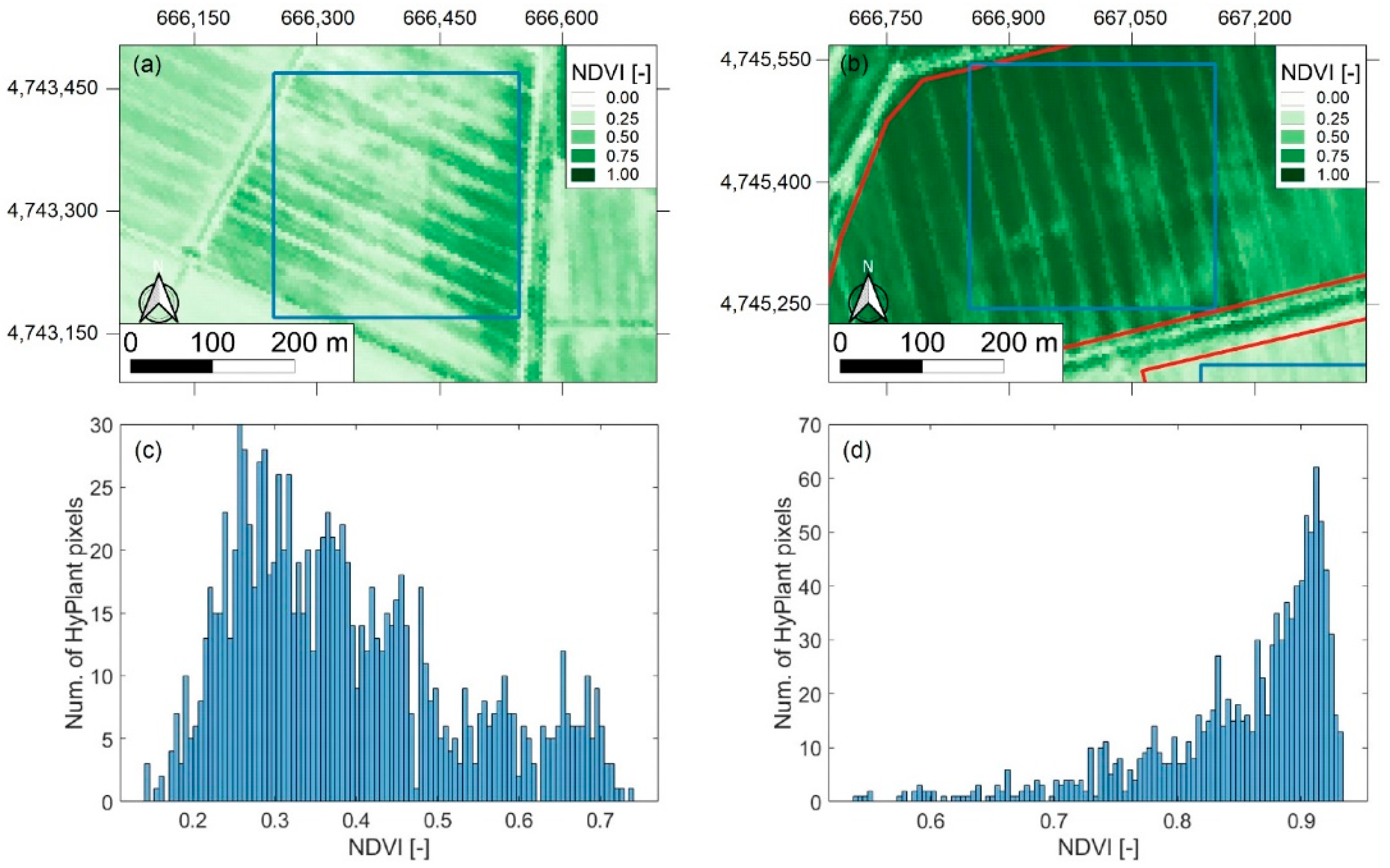
2.1. Study Area

Airborne data were collected in the summer of 2018 during the ESA-funded FLEXSense 2018 campaign from two test sites, “Selhausen” (Germany) and “Braccagni” (Italy).
The “Selhausen” study area (50.864N, 6.452E; elevation, 103 m above sea level) is located in the Rur catchment in the central western part of North Rhine-Westphalia (Germany). The Rur catchment is an intensive study area of the Transregional Collaborative Research Centre 32 [30]. The area is characterised by an agricultural landscape dominated by sugar beet, maize, rapeseed and potatoes. An area of approximately 10 km × 15 km was covered by the airborne imagery exploited in this study. Land-use classification was derived from supervised, multitemporal Sentinel-2 data. To enhance the land-use product, the multi-data approach was applied using information from the Authorative Topographic Cartographic Information System (ATKIS Basis DLM), Physical Block information, and OpenStreetMap [31,32].The “Braccagni” study area (42.830N, 11.070E; elevation, 2 m above sea level) is located 15 km from the coastline in central Tuscany (Italy). An area of approximately 6 km × 9 km characterised by a patchy agricultural landscape was covered by the airborne imagery exploited in this study. During summer, a variety of crops is grown in the area (e.g., corn, alfalfa, wheat, barley and chickpea). The land cover map at the time of the HyPlant acquisition was provided by the farmers and verified with field surveys. The size of the agricultural fields in the area varies considerably, ranging from small rain-fed patches to large, homogeneous fields irrigated with centre-pivot irrigation systems.

2.2. Airborne Data Preprocessing and Fluorescence Retrieval

Hyperspectral images were acquired over both sites using the HyPlant airborne imaging spectrometer developed by Forschungszentrum Jülich in cooperation with Specim Ltd. (Oulu, Finland) [33,34]. Airborne imagery was collected on 26 June 2018 and on 30 July 2018 in Selhausen and Braccagni, respectively. HyPlant is a line-imaging push-broom scanner consisting of two modules: (i) a fluorescence imager (FLUO) covering the red and far-red spectral regions (670–780 nm) at ultra-fine spectral resolution (FWHM ≃ 0.25 nm, SSI of 0.11 nm) for fluorescence retrieval and (ii) a dual-channel imager (DUAL) covering the visible (VIS), near-infrared (NIR) and shortwave infrared (SWIR) spectral regions (370–2500 nm) with an FWHM of 4.0 nm (VIS-NIR) to 13.3 nm (SWIR) for the reflectance calculation. Images were acquired at different flight altitudes varying between 1800 m and 3050 m above the surface, corresponding to a spatial resolution of 3 m and 4.5 m, respectively. All images were aggregated at a common spatial resolution of 9 m by means of averaging kernels. This spatial resolution was selected considering that an average sensor-target distance of 20 m, reasonable for UAS and tower-based systems installing point spectrometers with a conical field of view (usually 25 deg), would result in a projected circular field of view of ~9 m radius. Therefore, in this analysis, each sampling point corresponds to a 9 m × 9 m pixel within the HyPlant SIF maps.
The FLUO data were processed using a dedicated processing chain specifically developed to retrieve SIF with the spectral fitting methods (SFM [35]) adapted to HyPlant observations [36]. The SFM approach for airborne data consists of two main components: (i) atmospheric radiation transfer modelling and (ii) decoupling reflectance and fluorescence. Surface reflectance is modelled with polynomial splines and fluorescence with peak-like functions (i.e., Gaussian). MODTRAN-5 was used to calculate the atmospheric radiative transfer within the spectral windows corresponding to the O2 bands. To account for uncertainties in the description of the atmospheric state, an image-based approach was used to optimize the parameterization of the atmospheric radiative model. Instrument centre wavelength and bandwidth were characterised with the SpecCal algorithm [37], which was adapted for airborne data analysis. The retrieval of SIF within both O2 bands is based on an iterative optimization algorithm that matches at-sensor radiance spectra measured with HyPlant and forward modelled using the coupled surface–atmosphere radiative transfer equations. In this contribution, only SIF maps retrieved in the O2-A band at 760 nm will be considered in the analysis.
The DUAL data were atmospherically corrected with ATCOR-4 commercial software (Atmospheric and Topographic CORrection algorithm, ReSe Applications GmbH, Langeggweg, Switzerland) [38] to obtain top-of-canopy reflectance (TOC) as described by Siegman et al. [36]. Based on the TOC reflectance product, the normalised difference vegetation index (NDVI) was calculated as:
N D V I = R 795 810 R 665 680 R 795 810 + R 665 680
where R is the reflectance at the specified spectral windows corresponding to nine spectral bands of HyPlant (centre wavelength ±4 bands).
The coefficient of variation of NDVI was used to describe the spatial variability of plants within a field [39,40].

2.3. Selection of the Reference Areas

The overall framework for evaluation of the spatial representativeness of point SIF measurements and the uncertainty associated with spatial sampling on SIF map validation is described hereafter.
We determined the spatial representativeness of an increasing number of 9 × 9 m sampling points with respect to a defined reference area. The concept of sampling points at this scale can be considered equivalent to the results of traditional field spectroscopy measurements spatially distributed in the reference area or, likewise, measurements obtained from data collected with spectroradiometers onboard drones [41] or zip lines [42].
The selected reference areas in the Selhausen and Braccagni experimental sites correspond to (i) monocultural agricultural fields with variable size and (ii) 300 m × 300 m square areas representing hypothetical FLEX pixels visually drawn on the HyPlant maps. The FLEX pixels materialized on the images can include a variable number of land cover classes. Here, a perfect match between the in situ, airborne and satellite SIF values is assumed, selectively tackling only the uncertainty related to the spatial sampling (e.g., no uncertainty related to the retrieval, atmospheric correction or temporal mismatch).
Thirty-one monocultural agricultural fields were defined in the Selhausen area and 30 in the Braccagni study area. The boundaries of the selected fields were taken from a land cover map of the sites and integrated with manual digitization as necessary. The size of the monocultural fields ranged between 28,000 m2 and 97,000 m2, including bare soils, sugar beet, barley and pea fields in Selhausen, whereas the fields were much larger in Braccagni, ranging between 60,000 m2 and 300,000 m2, with wheat, barley and chickpea as the most represented land covers. For comparison, a FLEX pixel will sample an area of approximately 90,000 m2. For each field, the SIF average and standard deviation were computed.
In order to determine the influence of the pixel spatial heterogeneity (i.e., amount of land cover) on the representativeness of the point measurements for SIF validation, several 300 m × 300 m reference areas (corresponding to hypothetical FLEX pixels) were also positioned on the HyPlant maps in areas characterised by different land cover types. The selected reference areas include a maximum of 5 natural components (bare soils or vegetated land cover) within each 300 m × 300 m square. A land cover is considered in our analysis if its surface is equal or exceeds 5% of the hypothetical FLEX pixel area. As an example, Figure 1a shows the monocultural fields and FLEX pixels considered in the Braccagni study area.
For the Braccagni experimental site, a total of 39 FLEX pixels were identified. Among them, 18 are ‘pure’ pixels, meaning that they include only one component; 6 include two components; 11 comprise three components; and 4 have four components. For the Selhausen experimental site, a total of 11 FLEX pixels were placed: three with two components, six with three components and two with four components. The Braccagni and Selhausen areas have different characteristics, with Braccagni characterised by broad fields, allowing for the realization of one-component reference areas, whereas Selhausen is characterised by narrow fields, making the identification of one-component reference areas quite difficult. This explains the varying number of pixels selected in the two study areas and the differing composition of the FLEX pixels. Reference areas were placed in areas where the land covers were known (data not shown) at the time of the HyPlant overpass.
Then, we evaluated the impact of different sampling approaches on the capability of in situ measurements to be representative for a given reference area of both monocultural fields and FLEX-like pixels.

2.4. Data Sampling Strategy

The minimum number of sampling points needed to be representative of the SIF average value of the considered reference area was selected based on the methodology described hereafter.
First, a database of sampling points was created according to the following approach. In the monocultural fields and in the 300 m × 300 m square areas representing hypothetical FLEX pixels, 200 fully random sampling points were selected to simulate a random spatial sampling (Figure 1b). These random points are a minimum distance of 10 m from one another to avoid multiple sampling of the same pixel (Figure 1b). In areas with more than one land cover class, as many as 200 fully random pixels were selected for each class (Figure 1b). In this case, a minimum distance of 10 m was maintained. If the spatial extent of a land cover class did not allow for selection of 200 HyPlant pixels, a lower number was selected while still preserving the 10 m minimum distance.
Then, four sampling schemes with increasing complexity in terms of required ancillary information and weighting schemes were applied for the selection of the sampling points used in the following analyses:
  • Random sampling;
  • Random sampling with linear combination;
  • Stratified random sampling; and
  • Stratified random sampling with linear combination.
To reduce the number of combinations, a total of 73 sampling cases was created for each sampling scheme. The number of sampling points (npts) for each case varies between 1 and 200, with a step of 1 for cases with between 1 and 15 points, a step of 2 for cases with between 16 and 60 points and a step of 4 for cases with between 64 and 200 points. In order to avoid potential biases related to the random selection (i.e., when selecting by chance, a point “too close” or “too far” from the mean of the field), each case was repeated 200 times following a random resampling approach. The MATLAB randperm function was used for random selection, and within a single set of points (i.e., for each repetition), no replacement was allowed (each point selected a maximum one time), as it would not be realistic to measure the same point twice in the field, given time and resource constraints. The spatial representativeness of the sampled points with respect to the mean SIF value of each reference area was evaluated using the absolute deviation from the mean (ADM) computed as the absolute value of the difference between the mean SIF value of the sampled points ( μ S I F 760 p o i n t s ) and the mean value of the entire reference area ( μ S I F 760 r e f e r e n c e   a r e a ):
A D M = | μ S I F 760 p o i n t s μ S I F 760 r e f e r e n c e   a r e a |
ADM quantifies the absolute discrepancy in physical units between a satellite SIF observation and a given number of proximal sensing measurements performed to characterise the corresponding subtended surface.
ADM was then compared to three thresholds: T20 = 0.20 mWm−2 sr−1 nm−1, T15 = 0.15 mWm−2 sr−1 nm−1 and T10 = 0.10 mWm−2 sr−1 nm−1. The threshold T20 was selected considering that the ‘desired’ FLEX SIF level 2 product accuracy, for a reference fluorescence level of 2 mWm−2 sr−1 nm−1 at the emission peaks, is 0.2 mWm−2 sr−1 nm−1 (FLEX Mission Requirement Document, MRD [27]). The thresholds T15 and T10 were also considered because different sources of uncertainty can impact the final SIF estimates; thus, the uncertainty related to the spatial representativeness of in situ SIF observations should be lower than the value stated in the MRD (0.2 mWm−2 sr−1 nm−1).
As an example, Figure 2a shows the A D M values obtained for five (out of 200) sampling repetitions for one of the monocultural fields. For each of the 200 repetitions, the number of sampling points for which ADM was lower than T20, T15 or T10 was extracted. The distribution of these values for the reference area considered as an example is shown in Figure 2b–d. Starting from these distributions, the 95th percentile for each threshold was computed.
The ADM calculation was adapted to the different sampling schemes as described in the following paragraphs.

2.4.1. Random Sampling

The random sampling approach was applied to both the monocultural fields and the 300 m × 300 m square areas representing hypothetical FLEX pixels. The latter areas can include a number of land cover classes (between 1 and 4). The absolute deviation for the random sampling approach (ADMrs) was computed as:
A D M r s = | n = 1 n p t s S I F 760 , n p o i n t s n p t s μ S I F 760 r e f e r e n c e   a r e a |
where npts is the number of sampling points and varies from 1 to 200, and n is the nth point within the selected sample.

2.4.2. Random Sampling with Linear Combination

Given the potential mixture of different land cover types within a FLEX pixel in, e.g., agricultural landscapes, a linear combination model was applied to the sampled values. In this case, ADMrslm was computed as:
A D M r s l m = | μ S I F 760 p o i n t s l m i x μ S I F 760 r e f e r e n c e   a r e a |
where:
μ S I F 760 p o i n t s l i n = ( n = 1 n l c f c l c , n * μ S I F 760 , n p o i n t s ) + ( 1 n = 1 n l c f c l c , n ) * n = 1 n l c μ S I F 760 , n p o i n t s n l c
where μ S I F 760 p o i n t s l i n is the mean SIF value of the sampled points weighted according to the fractional cover of the land cover to which they belong, and μ S I F 760 r e f e r e n c e   a r e a is the mean SIF value of the entire reference area. nlc is the number of effective land covers within the reference area (i.e., the number of land cover components within a FLEX pixel that are sampled for each sampling case), and fclc is the fractional cover of each land cover within the reference area. In the first half of Equation (4), a linear model based on fclc was applied to the sampled values so that each group of points within a land cover was weighted for the fractional cover of the land cover in the FLEX pixel. Wherever one or more land covers are not included in the sampling (e.g., in cases with fewer sampling points than land covers), in the second half of Equation (4), a compensation factor is applied by multiplying the remaining fc by the average values of the sampled points. By combining Equations (3) and (4), the A D M for the data sampled with the linear combination model was computed.

2.4.3. Stratified Random Sampling (with and without Linear Combination)

In order to further improve the effectiveness of the spatial sampling of the FLEX pixel, a stratified random approach was tested with and without applying the linear combination to the selected points. The rationale followed to apply this scheme for varying number of sampling points (npts) and land covers within the FLEX pixel (nlc) is reported below.
  • nlc = 1, easiest case; points are selected incrementally for each case within the single land cover, and the linear combination is not applied;
  • nlc > 1 points are selected according to the following rules:
    npts = 1: the point is selected randomly among the points within the land cover with the highest fractional cover within the FLEX pixel;
    1 < nptsnlc: the points are selected randomly among the points within the land covers with the highest fractional cover within the FLEX pixel, i.e., if npts = 2 and nlc = 3, a single point for each land cover is selected among those within the two land covers with the highest fractional cover within the FLEX pixel;
    npts > nlc: the pixels are distributed among the different land covers proportionally to the fractional cover within the pixel of each land cover.
ADMsrs was computed using Equations (4) and (5).

3. Results

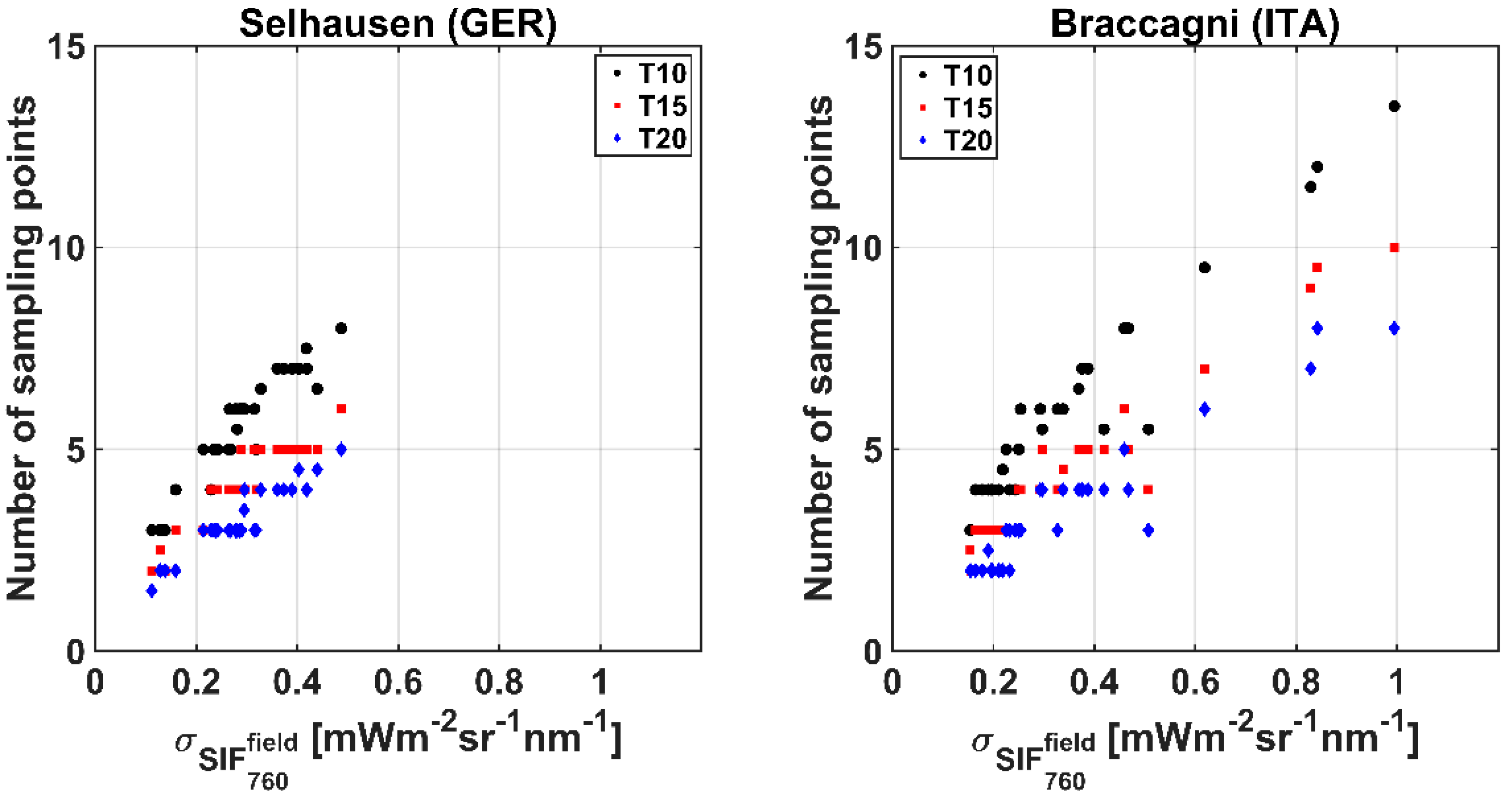
3.1. Impact of Increasingly Restrictive Thresholds on the Number of Sampling Points

Figure 3 shows the 95th percentile of the number of sampling points needed to meet the three thresholds defined in Section 2.4 for the monocultural fields in Selhausen and Braccagni experimental sites according to the random sampling approach. A positive relationship between the number of sampling points and the standard deviation of S I F 760 of each field ( σ S I F 760 f i e l d ) can be observed. The number of sampling points progressively increases for more restrictive thresholds (i.e., from T20 to T10). When considering T10 for both sites, a large variability in the number of sampling points can be observed from field to field, from a minimum of 3 to a maximum of 13.5 points, whereas 1.5 to 8 points are needed when considering T20. Therefore, the number of points to be sampled in the reference area increases with spatial variability, and the number of points increases as the uncertainty threshold decreases. In Braccagni, monocultural fields reach higher σ S I F 760 f i e l d values compared to Selhausen, but the overall linear relationship with the number of sampling points holds true across the entire range of σ S I F 760 f i e l d variation.
A similar pattern can be observed for the FLEX pixels at both sites (Figure 4), with a comparable number of sampling points needed to characterise pixels with a similar σ S I F 760 f i e l d value. In this case, all values are shown in relation to the standard deviation of S I F 760 of each FLEX pixel ( σ S I F 760 F L E X ).
For the sake of simplicity, only the more restrictive of the tested thresholds (T10 = 0.10 mWm−2 sr−1 nm−1) is shown in the following sections.

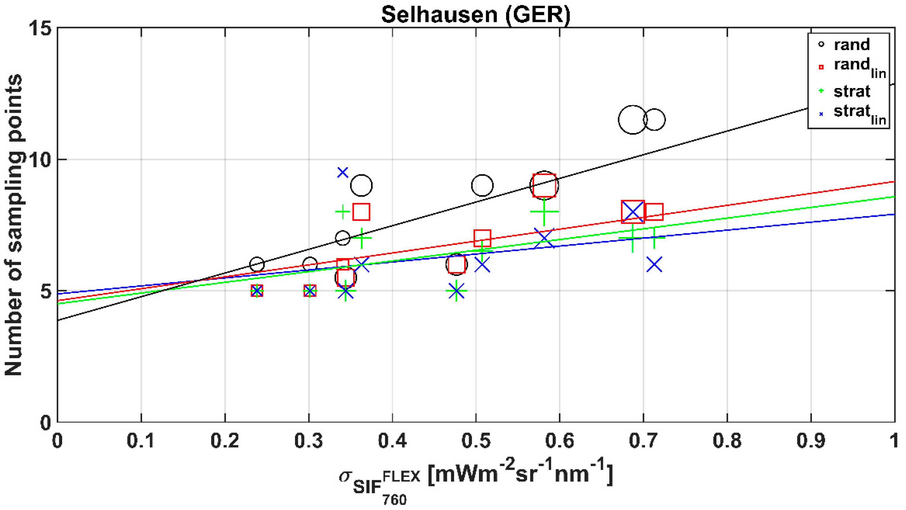
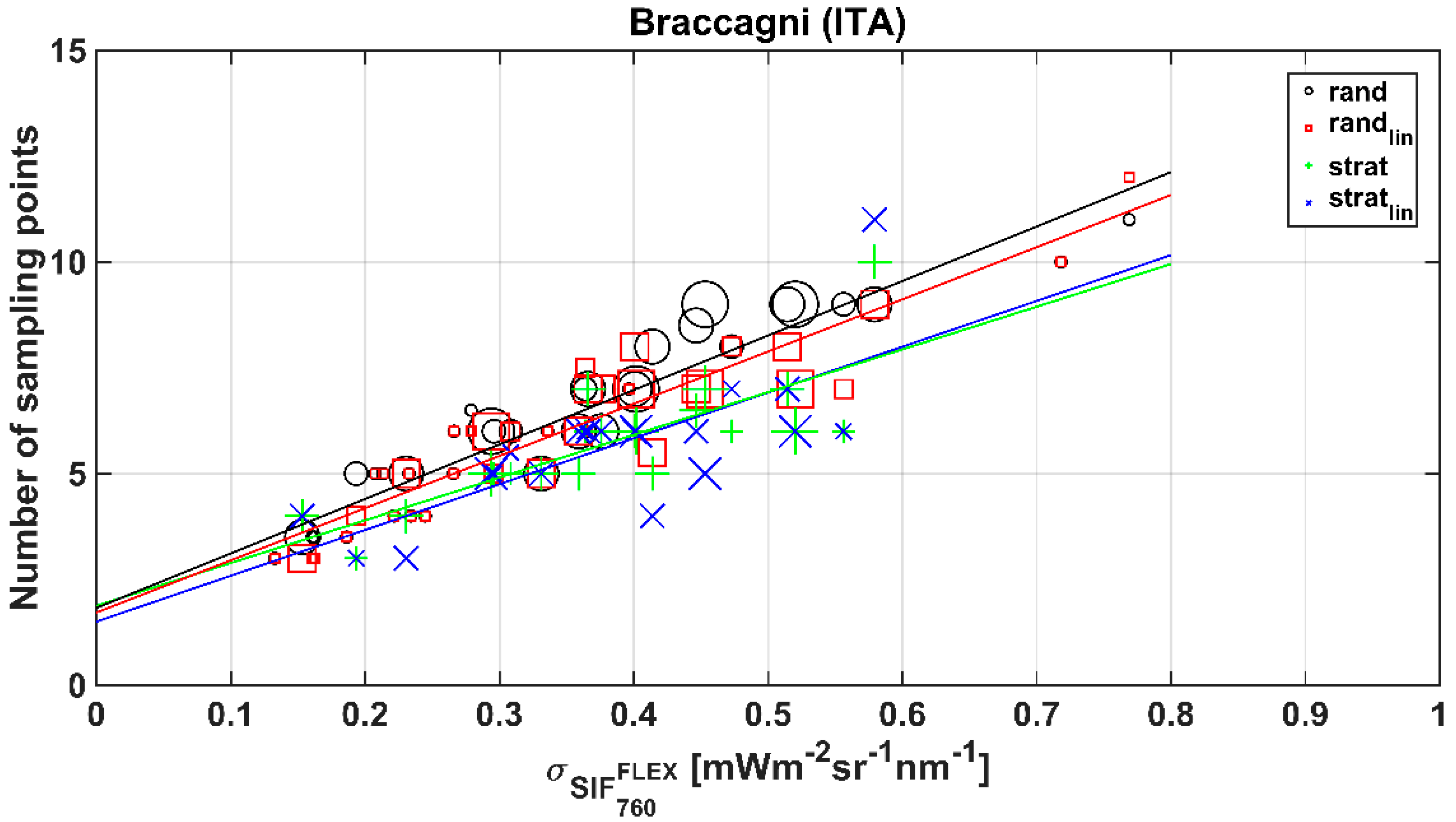
3.2. Impact of Proximal Sensing Sampling Schemes on the Number of Sampling Points in FLEX Pixels

The frequency distribution of the number of sampling points needed to meet the T10 threshold for all simulated sampling cases, aggregating data from all FLEX pixels in Selhausen and Braccagni (n = 10,000), is reported in Figure 5. Overall, the four sampling schemes described in Section 2.4 (i.e., random sampling, random sampling with a linear combination model, stratified random sampling and stratified random sampling with a linear combination model) show comparable results with respect to the aggregated data. Nevertheless, a shift toward a lower number of sampling points can be observed for the stratified sampling schemes (Figure 5c,d), with a discernibly higher frequency for cases in which two sampling points were sufficient to meet the T10 threshold. This can be explained by the fact that the sampling points were selected randomly among those within the land covers with the highest fractional cover within the FLEX pixel. Thus, we can expect the mean SIF value of the points sampled according to the stratified scheme to be closer to the mean SIF value of the entire FLEX pixel compared to the mean SIF value of randomly selected points.
On the other hand, sampling-specific patterns can be observed when analysing results from each FLEX pixel independently. Figure 6 and Figure 7 show the 95th percentile of the number of ground sampling points needed to meet the T10 thresholds for the FLEX pixels using different sampling approaches in the Selhausen and Braccagni experimental sites, respectively. All values are shown in relation to σ S I F 760 F L E X , whereas the pointer size is related to the number of components (i.e., land covers) within each FLEX pixel. The number of components varies from two to four in Selhausen and from one to four in Braccagni. Therefore, only at the Braccagni site is a FLEX-like homogeneous pixel with a single component observed.
Figure 6 and Figure 7 show the impact of the different sampling schemes on the number of sampling points needed to meet the threshold. Different approaches may produce different results. Overall, a decreasing number of sampling points is needed to characterise the FLEX pixel average SIF values for increasingly complex sampling schemes, as also highlighted by the decreasing slope of the linear OLS models (solid lines). In Selhausen, the largest differences occur when moving away from a random sampling scheme in favour of any of the more complex approaches (i.e., considering the land cover heterogeneity within the FLEX pixel). Although the stratified sampling schemes are generally the best-performing ones (i.e., meeting the threshold with a lower number of sampling points), the linear combination model for randomly selected sampling points shows noticeably better performance than the random selection alone. This is partially confirmed in Braccagni, particularly for FLEX pixels characterised by medium–high σ S I F 760 F L E X values (i.e., 0.4–0.6 mWm−2 sr−1 nm−1).
Figure 6 and Figure 7 also show that pixels with a higher number of components have generally higher σ S I F 760 F L E X values in Selhausen, although this behaviour is less predictable in Braccagni, possibly due to the larger fields and the higher intra-field SIF variability in the Braccagni reference areas.

3.3. Impact of Land cover Components on the Number of Sampling Points

Given the consistent results obtained in the two experimental sites and with the aim of establishing a more generalized approach, we aggregated the data from Braccagni and Selhausen to evaluate the impact of the number of components within each FLEX pixel for the different sampling strategies. Figure 8 shows a box plot of the 95th percentile of the number of sampling points needed to meet the T10 thresholds for all the FLEX pixels in both sites (i.e., aggregating data from Figure 6 and Figure 7). Groups “1”, “2”, “3” and “4” represent FLEX pixels with the corresponding number of land cover components. The impact of the number of components can be observed for the random sampling scheme (top left), with significant differences between group “1” and groups “3” and “4” (Kruskall–Wallis test, p < 0.05) but not between group “2” and any other group or between groups “3” and “4”. When using a random sampling approach combined with a linear combination (top right), there is a significant difference only between groups “1” and “4” (p < 0.05), with no significant impact of the number of land cover components observed for the stratified random sampling schemes (bottom left and right). Furthermore, σ S I F 760 F L E X values from group “1” are significantly lower than those for groups “3” and “4” (p < 0.05; data not shown), highlighting the link between intra-pixel SIF heterogeneity and the number of land cover classes within a pixel. This means that for pixels consisting of one land cover, at least 5 sampling points are needed to satisfy the T10 threshold, and overall, fewer than 15 points is theoretically enough to characterise the reference area in case of multicomponent conditions. Thus, even at sites characterised by greater complexity, if the appropriate sampling scheme is applied, relatively few measurements may be sufficient to characterise the SIF average value of the reference areas.
As observed in Figure 6 and Figure 7, high σ S I F 760 F L E X   values are not always related to the number of land cover classes within each pixel. This can be further appreciated in Figure 9, which shows a box plot of the coefficient of variation of NDVI with respect to the number of land cover components for all the FLEX pixels in both sites.
A general increase in the intra-pixel variability with the number of components is observed; however, the variability of the CV of NDVI within each group is quite high. This means that cases may occur in which the intra-pixel variability is relatively high, even if they are characterised by a single land cover class. For example, this happens for two FLEX pixels in Braccagni that show relatively high σ S I F 760 F L E X   values and characterised by a single land cover class with the highest number of sampling points. Figure 10 shows the NDVI (upper panels) maps of these two FLEX pixels characterised by corn under two different conditions. A significant spatial heterogeneity of the vegetated surface within the pixel can be observed for both pixels, showing discontinuous soil patches and major variations in greenness.

4. Discussion

An uncertainty budget related to SIF retrieval was recently provided by Buman et al. [12], who characterised the uncertainties due to instrumental effects, procedures applied for data calibration, atmospheric correction, SIF retrieval approach and the spatial representativeness of in situ observations compared to satellite measurements. Regarding the uncertainties related to the spatial representativeness, they pointed out the challenge of identifying pseudo-invariant homogeneous calibration sites for SIF products and the potential impact of site heterogeneity on the reliability of in situ SIF retrieval for satellite products validation.
In this paper, we moved a step forward, proposing an operational data-driven approach to quantitatively characterise the representativeness of a set of validation measurements within a reference area for the implementation of an SIF ground validation network. We exploited real airborne HyPlant data and well-established and widely used field sampling strategies to provide a quantitative indication of the number of in situ observations that may be needed to capture the average SIF of a reference area (e.g., future FLEX pixel in agricultural landscapes) within a given threshold.
A positive relationship between the minimum number of sampling points and the standard deviation of S I F 760 of each reference area (either field or pixel) is observed, highlighting the importance of selecting a homogeneous validation site to maintain a relatively low number of sampling points. As expected, the number of sampling points progressively increases for more restrictive thresholds (i.e., from T20 to T10). T20 corresponds to the FLEX SIF level 2 product accuracy for a reference fluorescence level of 2 mWm−2 sr−1 nm−1 at the emission peaks, as specified in the FLEX Mission Requirement Document (MRD [43]).
The choice of the sampling scheme has a minimal overall effect, showing similar results when considering aggregated data. Nevertheless, some recommendations can be drawn when analysing each pixel independently. In particular, if the reference areas are homogeneous in terms of SIF (low standard deviation), then all the tested sampling methods can perform well. Otherwise, sampling strategies that consider a stratification based on relevant spatially explicit layers are recommended.
Results from this study also show that prior knowledge of the land cover classes and extension within each FLEX pixel may not be sufficient to determine the number of sampling points, and concurrent information on the intra-class SIF variability must be considered. Thus, one limit of the proposed approach may be related to the need for systematic acquisitions of high-spatial-resolution SIF maps in order to define the best sampling approach for each validation site. Furthermore, the best sampling approach may vary over time due to changes in land cover type or crop phenological stage within the reference area for SIF validation (e.g., FLEX pixel). One possibility to overcome this issue is to characterise site homogeneity considering the spatial variability of the remote sensing indices that were found to correlate with SIF under unstressed conditions, such as NIRv and NIRvR [44,45]. The advantage of these VIs is that they can be systematically computed from high-temporal and -spatial-resolution satellite missions, such as the ESA Sentinel-2 mission. Future studies should create a planning scheme that seeks to maximize UAS coverage over the most variable areas for optimal fluorescence mapping using, for example, an adaptive scheme based on multitemporal Sentinel-2 images.
Despite efforts to define an optimised spatial sampling within the satellite pixel that is subject of a validation process, the intrinsic spatial scale mismatch between the measurements acquired from a spaceborne and ground-based platform directly translates into a geolocation mismatch, which can be a significant source of errors for highly dynamic parameters [11]. This aspect is not evaluated in this paper, but future studies are needed to quantify the collocation mismatch error and assess its impact on SIF product validation. Another point that is not addressed in this paper is the evaluation of the spatial variability at different wavelengths. Here, we consider the far-red SIF only, although we are aware that the spatial and temporal behaviour of fluorescence at other wavelengths may differ.
Once the number of measurements necessary to capture SIF variability has been defined, such an approach can be implemented using, for example, UAS platforms equipped with high-spectral-resolution point spectrometers. UAS data can replace traditional field spectroscopy measurements when there is a need to cover modest to large areas quickly [46], in particular when operated at a certain height above the target without the need to apply atmospheric compensation corrections [47]. However, a critical aspect for the validation of satellite products with UAS acquisitions is the current lack of consistency and interoperability of UAS data. Future efforts need to be directed toward guaranteeing quality-assured data from UAS, encouraging coordinated and harmonised processes and activities that enable interoperability, such as the Fiducial Reference Measurements for Vegetation (FRM4VEG) project initiated by ESA. A sampling strategy based on drone platforms is particularly relevant in coarse pixels, which should be sampled quickly because fluorescence is an instantaneous process that changes during the day. The typical flight speeds of multirotor UAS systems are around 5–10 m/s, and the flight duration is typically around 15–30 min for battery-operated UAS [48]. Thus, operating a high-resolution spectrometer for SIF measurement equipped with a 25° optic on a UAS flying at 20 m, about 20 points can be reasonably sampled distributed in 300 m × 300 m in 20 min. Taking into account that the FLEX satellite will cross the equator at around 10:00 [43], the SIF signal can be considered relatively stable during the 20 min (i.e., 10 min before and 10 min after the satellite overpass) needed to complete the acquisition in most areas of the world and for most times of the year when plants are photosynthetically active. However, whereas the quality and interoperability of satellite data are ensured by the Committee on Earth Observation Satellites (CEOS), the quality and accuracy of UAS data may depend on the type of sensor used, as well as the data acquisition and calibration procedures. These can vary among users and sensors, making multisource data interoperability difficult. Ensuring the consistency and interoperability of UAS data is an important challenge if they are to be used for satellite product validation [49]. UAS configuration, protocol and guidelines for fluorescence validation are still in early stages of development.
In summary, given the flexibility of the proposed data-driven approach, different sampling strategies and measurement footprints could be tested based on emerging needs and the evolution of the calibration and validation strategy for the FLEX products. Moreover, this methodology could be scaled to lower-spatial-resolution SIF products (e.g., TROPOMI SIF [50] and OCO-2 SIF [3]) and to other ecosystems (e.g., mixed and monospecific forests, tree–grass ecosystems and natural grasslands) to build a consistent strategy for SIF sampling and validation at different spatial scales.

5. Conclusions

Appropriate identification of the ground sampling approach in the FLEX configuration remains to be defined and optimized. To this end, different platforms and instruments can be exploited. However, the sampling approach also depends on the target type. In this study, we presented a statistical analysis (over different agricultural landscapes) focused on the understanding of the number of sampling points needed to meet three SIF uncertainty thresholds.
The spatial scale mismatch between satellite-pixel and point field measurements is a significant challenge impacting the accuracy assessment of SIF satellite products. Comparing in situ observations that sample a small footprint with satellite values derived on a pixel scale can be meaningful only when this mismatch is reduced. In this study, we proposed a method to evaluate the spatial representativeness of in situ SIF observations compared to medium-resolution SIF products, providing useful insights for the selection of the validation site network and particularly for the definition of the most effective sampling scheme for each site. The proposed approach can be implemented with currently available spectral systems, for example, by installing different instruments on the ground or by using high-spectral-resolution spectrometers installed on a UAS.
Overall, the contribution of this work is to establish guidelines and common protocols for cal/val of satellite sensor products. It is not limited to the validation of FLEX SIF products but can be easily extended to SIF products derived from different satellite platforms or to other land optical satellite sensors.

Author Contributions

Conceptualization, M.R., M.C. and R.C.; methodology, M.R., M.C. and M.M.; formal analysis, M.R., M.C. and G.B.; investigation, M.R., M.C. and G.B.; software, M.C.; data curation, S.C. and U.R.; writing—original draft preparation, M.R. and M.C.; writing—review and editing, all authors; visualization, M.C. and G.B.; funding acquisition, R.C. All authors have read and agreed to the published version of the manuscript.

Funding

We gratefully acknowledge the financial support of the European Space Agency (ESA) for airborne data acquisition within the framework of the FLEXSense campaign (ESA/Contract No. 4000125402/18/NL/NA). Marco Celesti was supported by a Living Planet Fellowship of the European Space Agency (ESA/Contract No. 4000125442/18/I-NS). This work was partially funded by the Deutsche Forschungsgemeinschaft (DFG, German Research Foundation) under Germany’s Excellence Strategy (EXC 2070–390732324).

Data Availability Statement

The data presented in this study are available upon request from the corresponding author. HyPlant data are available from the ESA campaign data repository or upon request from U. Rascher. Land use classification for the Selhausen area was provided by Ulrike Lussem and Marina Herbrecht and is available at doi: 10.5880/TR32DB.38. Open data access is supported by the Deutsche Forschungsgemeinschaft (DFG, German Research Foundation) (491111487).

Acknowledgments

The authors are thankful to Dirk Schüttemeyer (European Space Agency) for the coordination of the FLEXSense campaign and to Matthias Drusch and FLEX MAG members for feedback during early stages.

Conflicts of Interest

The authors declare no conflict of interest.

References

  1. Baker, N.R. Chlorophyll Fluorescence: A Probe of Photosynthesis in Vivo. Annu. Rev. Plant Biol. 2008, 59, 89–113. [Google Scholar] [CrossRef] [PubMed] [Green Version]
  2. Zhang, Y.; Migliavacca, M.; Penuelas, J.; Ju, W. Advances in Hyperspectral Remote Sensing of Vegetation Traits and Functions. Remote Sens. Environ. 2021, 252, 1–5. [Google Scholar] [CrossRef]
  3. Joiner, J.; Guanter, L.; Lindstrot, R.; Voigt, M.; Vasilkov, A.P.; Middleton, E.M.; Huemmrich, K.F.; Yoshida, Y.; Frankenberg, C. Global Monitoring of Terrestrial Chlorophyll Fluorescence from Moderate-Spectral-Resolution near-Infrared Satellite Measurements: Methodology, Simulations, and Application to GOME-2. Atmos. Meas. Tech. 2013, 6, 2803–2823. [Google Scholar] [CrossRef] [Green Version]
  4. Joiner, J.; Yoshida, Y.; Guanter, L.; Middleton, E.M. New Methods for the Retrieval of Chlorophyll Red Fluorescence from Hyperspectral Satellite Instruments: Simulations and Application to GOME-2 and SCIAMACHY. Atmos. Meas. Tech. 2016, 9, 3939–3967. [Google Scholar] [CrossRef] [Green Version]
  5. Köhler, P.; Frankenberg, C.; Magney, T.S.; Guanter, L.; Joiner, J.; Landgraf, J. Global Retrievals of Solar-Induced Chlorophyll Fluorescence With TROPOMI: First Results and Intersensor Comparison to OCO-2. Geophys. Res. Lett. 2018, 45, 10456–10463. [Google Scholar] [CrossRef] [Green Version]
  6. Sun, Y.; Frankenberg, C.; Jung, M.; Joiner, J.; Guanter, L.; Köhler, P.; Magney, T. Overview of Solar-Induced Chlorophyll Fluorescence (SIF) from the Orbiting Carbon Observatory-2: Retrieval, Cross-Mission Comparison, and Global Monitoring for GPP. Remote Sens. Environ. 2018, 209, 808–823. [Google Scholar] [CrossRef]
  7. Du, S.; Liu, L.; Liu, X.; Zhang, X.; Zhang, X.; Bi, Y.; Zhang, L. Retrieval of Global Terrestrial Solar-Induced Chlorophyll Fluorescence from TanSat Satellite. Sci. Bull. 2018, 63, 1502–1512. [Google Scholar] [CrossRef] [Green Version]
  8. Drusch, M.; Moreno, J.; del Bello, U.; Franco, R.; Goulas, Y.; Huth, A.; Kraft, S.; Middleton, E.M.; Miglietta, F.; Mohammed, G.; et al. Concept—ESA’s Earth Explorer 8. IEEE Trans. Geosci. Remote Sens. 2017, 55, 1273–1284. [Google Scholar] [CrossRef]
  9. Guillevic, P.C.; Biard, J.C.; Hulley, G.C.; Privette, J.L.; Hook, S.J.; Olioso, A.; Göttsche, F.M.; Radocinski, R.; Román, M.O.; Yu, Y.; et al. Validation of Land Surface Temperature Products Derived from the Visible Infrared Imaging Radiometer Suite (VIIRS) Using Ground-Based and Heritage Satellite Measurements. Remote Sens. Environ. 2014, 154, 19–37. [Google Scholar] [CrossRef]
  10. Morisette, J.T.; Baret, F.; Privette, J.L.; Myneni, R.B.; Nickeson, J.E.; Garrigues, S.; Shabanov, N.V.; Weiss, M.; Fernandes, R.A.; Leblanc, S.G.; et al. Validation of Global Moderate-Resolution LAI Products: A Framework Proposed within the CEOS Land Product Validation Subgroup. IEEE Trans. Geosci. Remote Sens. 2006, 44, 1804–1814. [Google Scholar] [CrossRef]
  11. Niro, F.; Goryl, P.; Dransfeld, S.; Boccia, V.; Gascon, F.; Adams, J.; Themann, B.; Scifoni, S.; Doxani, G. European Space Agency (Esa) Calibration/Validation Strategy for Optical Land-Imaging Satellites and Pathway towards Interoperability. Remote Sens. 2021, 13, 3003. [Google Scholar] [CrossRef]
  12. Buman, B.; Hueni, A.; Colombo, R.; Cogliati, S.; Celesti, M.; Julitta, T.; Burkart, A.; Siegmann, B.; Rascher, U.; Drusch, M.; et al. Towards Consistent Assessments of in Situ Radiometric Measurements for the Validation of Fluorescence Satellite Missions. Remote Sens. Environ. 2022, 274, 112984. [Google Scholar] [CrossRef]
  13. Julitta, T.; Corp, L.A.; Rossini, M.; Burkart, A.; Cogliati, S.; Davies, N.; Hom, M.; Arthur, A.M.; Middleton, E.M.; Rascher, U.; et al. Comparison of Sun-Induced Chlorophyll Fluorescence Estimates Obtained from Four Portable Field Spectroradiometers. Remote Sens. 2016, 8, 122. [Google Scholar] [CrossRef] [Green Version]
  14. Porcar-Castell, A.; Mac Arthur, A.; Rossini, M.; Eklundh, L.; Pacheco-Labrador, J.; Anderson, K.; Balzarolo, M.; Martín, M.P.; Jin, H.; Tomelleri, E.; et al. EUROSPEC: At the Interface between Remote-Sensing and Ecosystem CO2 Flux Measurements in Europe. Biogeosciences 2015, 12, 6103–6124. [Google Scholar] [CrossRef] [Green Version]
  15. Cendrero-Mateo, M.P.; Wieneke, S.; Damm, A.; Alonso, L.; Pinto, F.; Moreno, J.; Guanter, L.; Celesti, M.; Rossini, M.; Sabater, N.; et al. Sun-Induced Chlorophyll Fluorescence III: Benchmarking Retrieval Methods and Sensor Characteristics for Proximal Sensing. Remote Sens. 2019, 11, 962. [Google Scholar] [CrossRef] [Green Version]
  16. Balzarolo, M.; Anderson, K.; Nichol, C.; Rossini, M.; Vescovo, L.; Arriga, N.; Wohlfahrt, G.; Calvet, J.-C.; Carrara, A.; Cerasoli, S.; et al. Ground-Based Optical Measurements at European Flux Sites: A Review of Methods, Instruments and Current Controversies. Sensors 2011, 11, 7954–7981. [Google Scholar] [CrossRef]
  17. Biriukova, K.; Pacheco-Labrador, J.; Migliavacca, M.; Mahecha, M.D.; Gonzalez-Cascon, R.; Martín, M.P.; Rossini, M. Performance of Singular Spectrum Analysis in Separating Seasonal and Fast Physiological Dynamics of Solar-Induced Chlorophyll Fluorescence and PRI Optical Signals. J. Geophys. Res. Biogeosciences 2021, 126, 1–25. [Google Scholar] [CrossRef]
  18. Martini, D.; Sakowska, K.; Wohlfahrt, G.; Pacheco-Labrador, J.; van der Tol, C.; Porcar-Castell, A.; Magney, T.S.; Carrara, A.; Colombo, R.; El-Madany, T.S.; et al. Heatwave Breaks down the Linearity between Sun-Induced Fluorescence and Gross Primary Production. New Phytol. 2022, 233, 2415–2428. [Google Scholar] [CrossRef]
  19. Grossmann, K.; Frankenberg, C.; Magney, T.S.; Hurlock, S.C.; Seibt, U.; Stutz, J. PhotoSpec: A New Instrument to Measure Spatially Distributed Red and Far-Red Solar-Induced Chlorophyll Fluorescence. Remote Sens. Environ. 2018, 216, 311–327. [Google Scholar] [CrossRef] [Green Version]
  20. MacArthur, A.; Robinson, I.; Rossini, M.; Davis, N.; MacDonald, K. Edinburgh Research Explorer A Dual-Field-of-View Spectrometer System for Reflectance and Fluorescence Measurements (Piccolo Doppio) and Correction of Etaloning Citation for Published Version: A DUAL-FIELD-OF-VIEW SPECTROMETER SYSTEM FOR REFLECTANCE AND FL. In Proceedings of the Fifth International Workshop on Remote Sensing of Vegetation Fluorescence, Paris, France, 22–24 April 2014; pp. 1–8. [Google Scholar]
  21. Cendrero-Mateo, M.P.; Bennertz, S.; Burkart, A.; Julitta, T.; Cogliati, S.; Scharr, H.; Rademske, P.; Alonso, L.; Pinto, F.; Rascher, U. Sun Induced Fluorescence Calibration and Validation for Field Phenotyping. Int. Geosci. Remote Sens. Symp. 2018, 2018-July, 8248–8251. [Google Scholar] [CrossRef]
  22. Gu, L.; Han, J.; Wood, J.D.; Chang, C.Y.Y.; Sun, Y. Sun-Induced Chl Fluorescence and Its Importance for Biophysical Modeling of Photosynthesis Based on Light Reactions. New Phytol. 2019, 223, 1179–1191. [Google Scholar] [CrossRef] [PubMed] [Green Version]
  23. Gautam, D.; Lucieer, A.; Bendig, J.; Malenovsky, Z. Footprint Determination of a Spectroradiometer Mounted on an Unmanned Aircraft System. IEEE Trans. Geosci. Remote Sens. 2020, 58, 3085–3096. [Google Scholar] [CrossRef]
  24. Garzonio, R.; di Mauro, B.; Colombo, R.; Cogliati, S. Surface Reflectance and Sun-Induced Fluorescence Spectroscopy Measurements Using a Small Hyperspectral UAS. Remote Sens. 2017, 9, 472. [Google Scholar] [CrossRef] [Green Version]
  25. Chang, C.Y.; Zhou, R.; Kira, O.; Marri, S.; Skovira, J.; Gu, L.; Sun, Y. An Unmanned Aerial System (UAS) for Concurrent Measurements of Solar-Induced Chlorophyll Fluorescence and Hyperspectral Reflectance toward Improving Crop Monitoring. Agric. For. Meteorol. 2020, 294, 108145. [Google Scholar] [CrossRef]
  26. Wang, N.; Suomalainen, J.; Bartholomeus, H.; Kooistra, L.; Masiliūnas, D.; Clevers, J.G.P.W. Diurnal Variation of Sun-Induced Chlorophyll Fluorescence of Agricultural Crops Observed from a Point-Based Spectrometer on a UAV. Int. J. Appl. Earth Obs. Geoinf. 2021, 96. [Google Scholar] [CrossRef]
  27. Zhang, X.; Zhang, Z.; Zhang, Y.; Zhang, Q.; Liu, X.; Chen, J.; Wu, Y.; Wu, L. Influences of Fractional Vegetation Cover on the Spatial Variability of Canopy SIF from Unmanned Aerial Vehicle Observations. Int. J. Appl. Earth Obs. Geoinf. 2022, 107, 102712. [Google Scholar] [CrossRef]
  28. Baret, F.; Weiss, M.; Allard, D.; Garrigues, S.; Leroy, M.; Jeanjean, H.; Fernandes, R.; Myneni, R.; Privette, J.; Morisette, J. VALERI: A Network of Sites and a Methodology for the Validation of Medium Spatial Resolution Land Satellite Products. Remote Sens. Environ. Is J. 2021, hal-03221068. [Google Scholar]
  29. Lv, T.; Zhou, X.; Tao, Z.; Sun, X.; Wang, J.; Li, R.; Xie, F. Remote Sensing-Guided Spatial Sampling Strategy over Heterogeneous Surface Ground for Validation of Vegetation Indices Products with Medium and High Spatial Resolution. Remote Sens. 2021, 13, 2674. [Google Scholar] [CrossRef]
  30. Simmer, C.; Thiele-Eich, I.; Masbou, M.; Amelung, W.; Bogena, H.; Crewell, S.; Diekkrüger, B.; Ewert, F.; Hendricks Franssen, H.J.; Huisman, J.A.; et al. Monitoring and Modeling the Terrestrial System from Pores to Catchments: The Transregional Collaborative Research Center on Patterns in the Soil-Vegetation-Atmosphere System. Bull. Am. Meteorol. Soc. 2015, 96, 1765–1787. [Google Scholar] [CrossRef] [Green Version]
  31. Waldhoff, G.; Lussem, U.; Bareth, G. Multi-Data Approach for Remote Sensing-Based Regional Crop Rotation Mapping: A Case Study for the Rur Catchment, Germany. Int. J. Appl. Earth Obs. Geoinf. 2017, 61, 55–69. [Google Scholar] [CrossRef]
  32. Lussem, U.; Herbrecht, M. Land use classification of 2018 for the Rur catchment. TR32DB 2019. [Google Scholar] [CrossRef]
  33. Rascher, U.; Alonso, L.; Burkart, A.; Cilia, C.; Cogliati, S.; Colombo, R.; Damm, A.; Drusch, M.; Guanter, L.; Hanus, J.; et al. Sun-Induced Fluorescence - a New Probe of Photosynthesis: First Maps from the Imaging Spectrometer HyPlant. Glob. Chang. Biol. 2015, 21, 4673–4684. [Google Scholar] [CrossRef] [PubMed] [Green Version]
  34. Rossini, M.; Nedbal, L.; Guanter, L.; Ač, A.; Alonso, L.; Burkart, A.; Cogliati, S.; Colombo, R.; Damm, A.; Drusch, M.; et al. Red and Far Red Sun-Induced Chlorophyll Fluorescence as a Measure of Plant Photosynthesis. Geophys. Res. Lett. 2015, 42, 1632–1639. [Google Scholar] [CrossRef] [Green Version]
  35. Cogliati, S.; Verhoef, W.; Kraft, S.; Sabater, N.; Alonso, L.; Vicent, J.; Moreno, J.; Drusch, M.; Colombo, R. Retrieval of Sun-Induced Fluorescence Using Advanced Spectral Fitting Methods. Remote Sens. Environ. 2015, 169, 344–357. [Google Scholar] [CrossRef]
  36. Siegmann, B.; Alonso, L.; Celesti, M.; Cogliati, S.; Colombo, R.; Damm, A.; Douglas, S.; Guanter, L.; Hanuš, J.; Kataja, K.; et al. The High-Performance Airborne Imaging Spectrometer HyPlant-from Raw Images to Top-of-Canopy Reflectance and Fluorescence Products: Introduction of an Automatized Processing Chain. Remote Sens. 2019, 11, 2760. [Google Scholar] [CrossRef] [Green Version]
  37. Meroni, M.; Busetto, L.; Guanter, L.; Cogliati, S.; Crosta, G.F.; Migliavacca, M.; Panigada, C.; Rossini, M.; Colombo, R. Characterization of Fine Resolution Field Spectrometers Using Solar Fraunhofer Lines and Atmospheric Absorption Features. Appl. Opt. 2010, 49, 2858–2871. [Google Scholar] [CrossRef] [Green Version]
  38. Richter, R.; Schlapfer, D. Geo-Atmospheric Processing of Airborne Imaging Spectrometry Data. Part 2: Atmospheric/Topographic Correction. Int. J. Remote Sens. 2002, 23, 2631–2649. [Google Scholar] [CrossRef]
  39. Govaerts, B.; Verhulst, N.; Sayre, K.D.; De Corte, P.; Goudeseune, B.; Lichter, K.; Crossa, J.; Deckers, J.; Dendooven, L. Evaluating Spatial within Plot Crop Variability for Different Management Practices with an Optical Sensor? Plant Soil 2007, 299, 29–42. [Google Scholar] [CrossRef]
  40. Scotford, I.M.; Miller, P.C.H. Estimating Tiller Density and Leaf Area Index of Winter Wheat Using Spectral Reflectance and Ultrasonic Sensing Techniques. Biosyst. Eng. 2004, 89, 395–408. [Google Scholar] [CrossRef]
  41. Vargas, J.Q.; Bendig, J.; Arthur, A.M.; Burkart, A.; Julitta, T.; Maseyk, K.; Thomas, R.; Siegmann, B.; Rossini, M.; Celesti, M.; et al. Unmanned Aerial Systems (UAS)-Based Methods for Solar Induced Chlorophyll Fluorescence (SIF) Retrieval with Non-Imaging Spectrometers: State of the Art. Remote Sens. 2020, 12, 1624. [Google Scholar] [CrossRef]
  42. Kirchgessner, N.; Liebisch, F.; Yu, K.; Pfeifer, J.; Friedli, M.; Hund, A.; Walter, A. The ETH Field Phenotyping Platform FIP: A Cable-Suspended Multi-Sensor System. Funct. Plant Biol. 2017, 44, 154–168. [Google Scholar] [CrossRef]
  43. ESA (European Space Agency). FLEX Earth Explorer 8 Mission Requirements Document, Version 3.0, Issue Date 05/06/2018; ESA Earth and Mission Science Division: Noordwijk, The Netherlands, 2018; Ref: ESAEOP- SM/2221/MDru-md. [Google Scholar]
  44. Zeng, Y.; Badgley, G.; Dechant, B.; Ryu, Y.; Chen, M.; Berry, J.A. A Practical Approach for Estimating the Escape Ratio of Near-Infrared Solar-Induced Chlorophyll Fluorescence. Remote Sens. Environ. 2019, 232, 111209. [Google Scholar] [CrossRef] [Green Version]
  45. Zeng, Y.; Chen, M.; Hao, D.; Damm, A.; Badgley, G.; Rascher, U.; Johnson, J.E.; Dechant, B.; Siegmann, B.; Ryu, Y.; et al. Combining Near-Infrared Radiance of Vegetation and Fluorescence Spectroscopy to Detect Effects of Abiotic Changes and Stresses. Remote Sens. Environ. 2022, 270, 112856. [Google Scholar] [CrossRef]
  46. Alvarez-Vanhard, E.; Corpetti, T.; Houet, T. UAV & Satellite Synergies for Optical Remote Sensing Applications: A Literature Review. Sci. Remote Sens. 2021, 3, 100019. [Google Scholar] [CrossRef]
  47. Sabater, N.; Vicent, J.; Alonso, L.; Verrelst, J.; Middleton, E.M.; Porcar-Castell, A.; Moreno, J. Compensation of Oxygen Transmittance Effects for Proximal Sensing Retrieval of Canopy-Leaving Sun-Induced Chlorophyll Fluorescence. Remote Sens. 2018, 10, 1551. [Google Scholar] [CrossRef] [Green Version]
  48. Nex, F.; Armenakis, C.; Cramer, M.; Cucci, D.A.; Gerke, M.; Honkavaara, E.; Kukko, A.; Persello, C.; Skaloud, J. UAV in the Advent of the Twenties: Where We Stand and What Is Next. ISPRS J. Photogramm. Remote Sens. 2022, 184, 215–242. [Google Scholar] [CrossRef]
  49. Lu, H.; Fan, T.; Ghimire, P.; Deng, L. Experimental Evaluation and Consistency Comparison of UAV Multispectral Minisensors. Remote Sens. 2020, 12, 2542. [Google Scholar] [CrossRef]
  50. Guanter, L.; Bacour, C.; Schneider, A.; Aben, I.; van Kempen, T.A.; Retscher, C.; Köhler, P.; Frankenberg, C.; Joiner, J. Sentinel-5P TROPOMI Mission. Earth Syst. Sci. Data 2021, 202104, 1–27. [Google Scholar] [CrossRef]
Figure 1. Monocultural fields and FLEX pixels considered in the Braccagni study area (a). Example of the realization of 200 fully random points within a monocultural field (orange dots) and within a hypothetical FLEX pixel (brown dots). Green diamonds show the 200 fully random points selected for each land cover in a FLEX pixel composed of two different components (b). The map projection is Universal Transverse of Mercator (UTM) zone 32N with datum WGS84 (World Geodetic System 1984).
Remotesensing 14 05107 g001
Figure 2. ADM values obtained for five sampling repetitions for one of the monocultural fields shown here as an example. n is the nth sampling repetition. Only five of the 200 sampling repetitions are shown for clarity of representation (a). Distribution of the number of sampling points for which the absolute deviation from the mean (ADM) was lower than T20 (b), T15 (c) or T10 (d).
Remotesensing 14 05107 g002
Figure 3. The 95th percentile of the number of sampling points needed to meet the three selected thresholds for the monocultural fields in Selhausen (Germany) and Braccagni (Italy) experimental sites using a random sampling approach.
Remotesensing 14 05107 g003
Figure 4. The 95th percentile of the number of sampling points needed to meet the thresholds for the FLEX pixels in Selhausen (Germany) and Braccagni (Italy) experimental sites using a random sampling approach.
Remotesensing 14 05107 g004
Figure 5. Distribution of the number of sampling points needed to meet the T10 threshold for all simulated cases (n = 10,000) aggregating data from all FLEX pixels in Selhausen (Germany) and Braccagni (Italy) experimental sites using a random sampling, a random sampling with a linear combination model, a stratified random sampling and a stratified random sampling with a linear combination model.
Remotesensing 14 05107 g005
Figure 6. The 95th percentile of the number of sampling points needed to meet the T10 thresholds for the FLEX pixels in Selhausen (Germany) experimental site using a random sampling, a random sampling with a linear combination model, a stratified random sampling and a stratified random sampling with a linear combination model. The number of sampling points is shown in relation to σ S I F 760 F L E X . The pointer size is related to the number of components within each FLEX pixel (2–4). The solid lines show the linear OLS regressions for each sampling strategy.
Remotesensing 14 05107 g006
Figure 7. The 95th percentile of the number of sampling points needed to meet the T10 thresholds for the FLEX pixels in Braccagni (Italy) experimental site using a random sampling, a random sampling with a linear combination model, a stratified random sampling and a stratified random sampling with a linear combination model. The number of sampling points is shown in relation to σ SIF 760 FLEX . The pointer size is related to the number of components within each FLEX pixel (1–3). The solid lines show the linear OLS regressions for each sampling strategy.
Remotesensing 14 05107 g007
Figure 8. Box plot of the 95th percentile of the number of sampling points needed to meet the T10 thresholds for all the FLEX pixels in both sites. Groups “1”, “2”, “3” and “4” represent FLEX pixels with the corresponding number of land cover components.
Remotesensing 14 05107 g008
Figure 9. Box plot of the coefficient of variation of NDVI for all the FLEX pixels in both sites. Groups “1”, “2”, “3” and “4” represent FLEX pixels with the corresponding number of land cover components.
Remotesensing 14 05107 g009
Figure 10. NDVI maps (a,b) and frequency distribution histograms (c,d) of two FLEX pixels characterised by a single land cover class and a high intra-pixel standard deviation of SIF 760 ( σ S I F 760 F L E X ). The map projection is UTM zone 32N with datum WGS84.
Remotesensing 14 05107 g010
Publisher’s Note: MDPI stays neutral with regard to jurisdictional claims in published maps and institutional affiliations.

