


Dynamic Monitoring of Environmental Quality in the Loess Plateau from 2000 to 2020 Using the Google Earth Engine Platform and the Remote Sensing Ecological Index

Abstract

1. Introduction
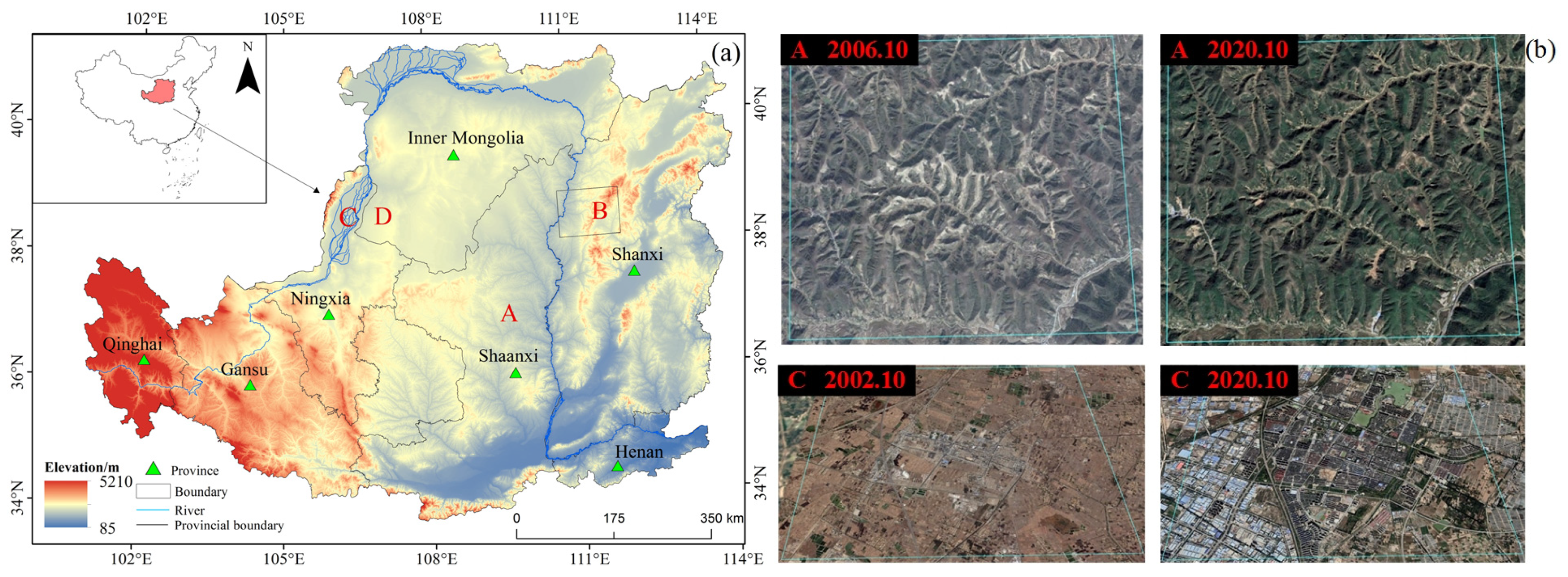
2. Study Area
3. Data and Methods
3.1. Data Sources and Processing
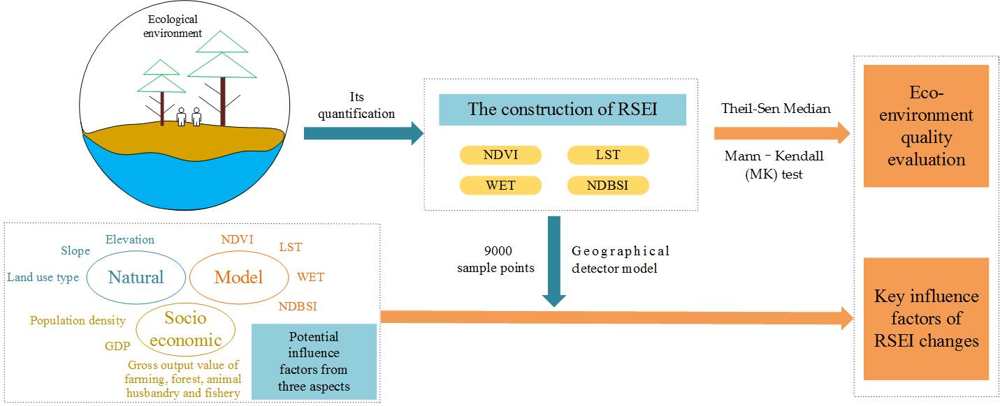
3.2. Research Methods
3.2.1. Calculation of RSEI
- (1)
- Normalized difference vegetation index
- (2)
- LST
- (3)
- Wetness
- (4)
- Normalized differential build-up and bare soil index
- (5)
- Normalization of the Measures
3.2.2. RSEI Trend Analysis
3.2.3. Analysis of Driving Forces Based on Geographic Detector
4. Results
4.1. Spatio-Temporal Variations Analysis of RSEI
4.1.1. PCA Analysis of RSEI Indicators
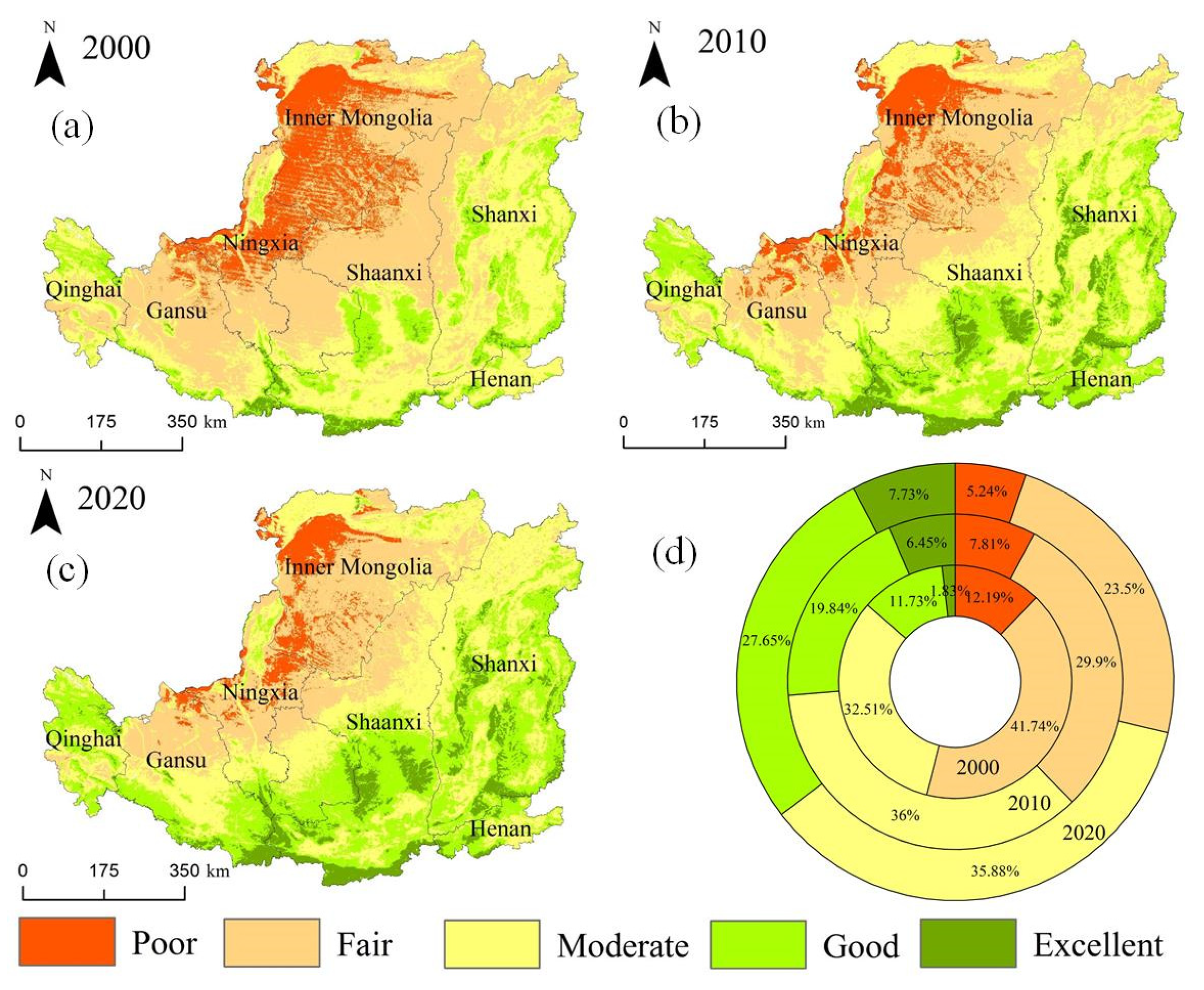
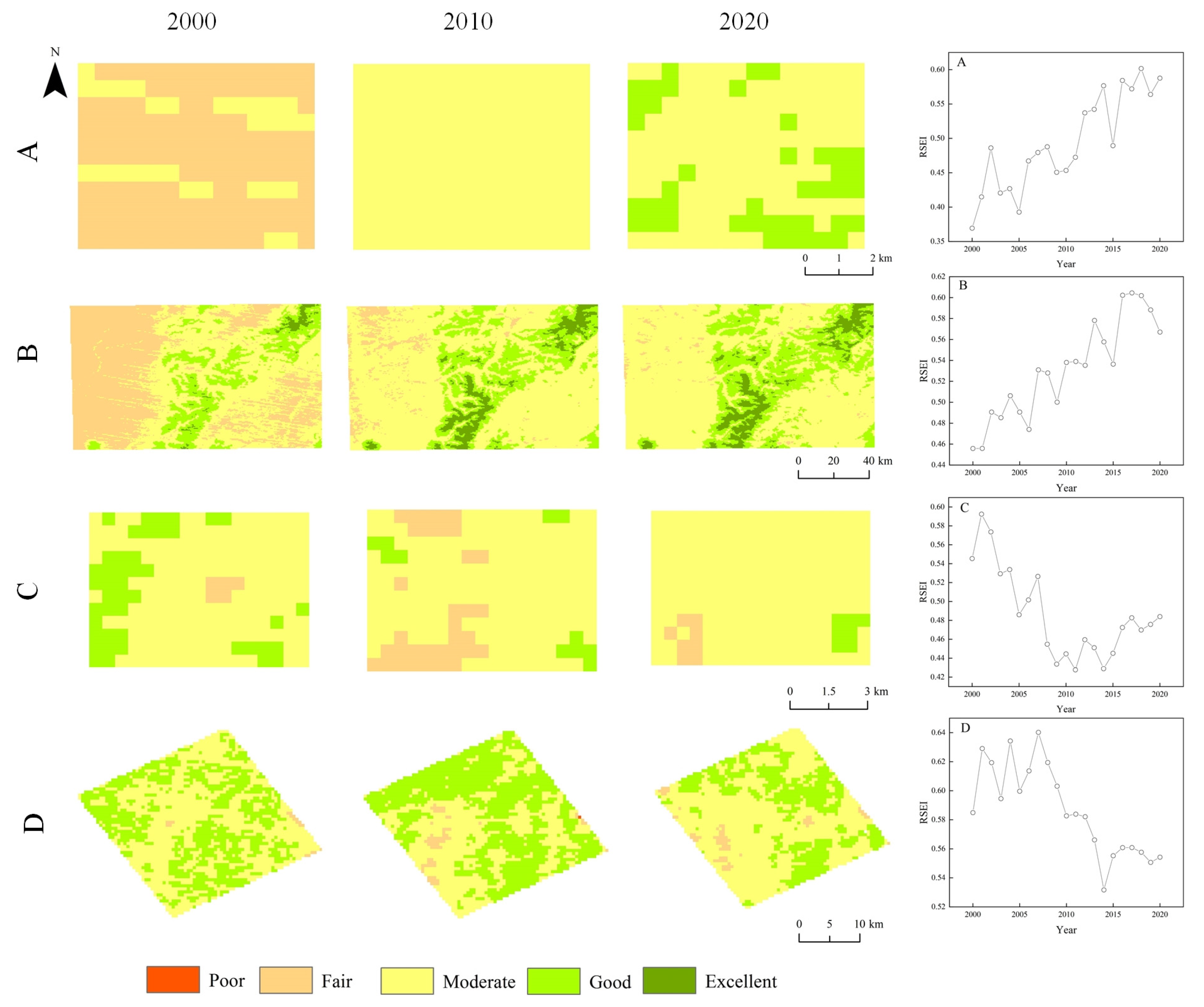
4.1.2. Spatiotemporal Changes of RSEI in the LP
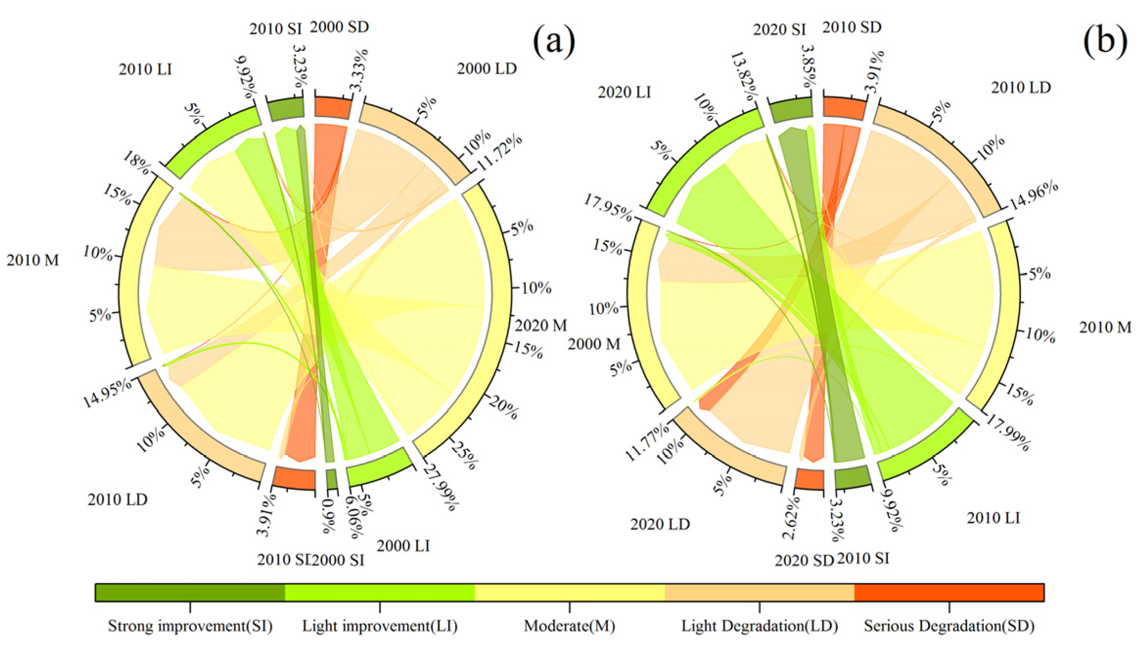
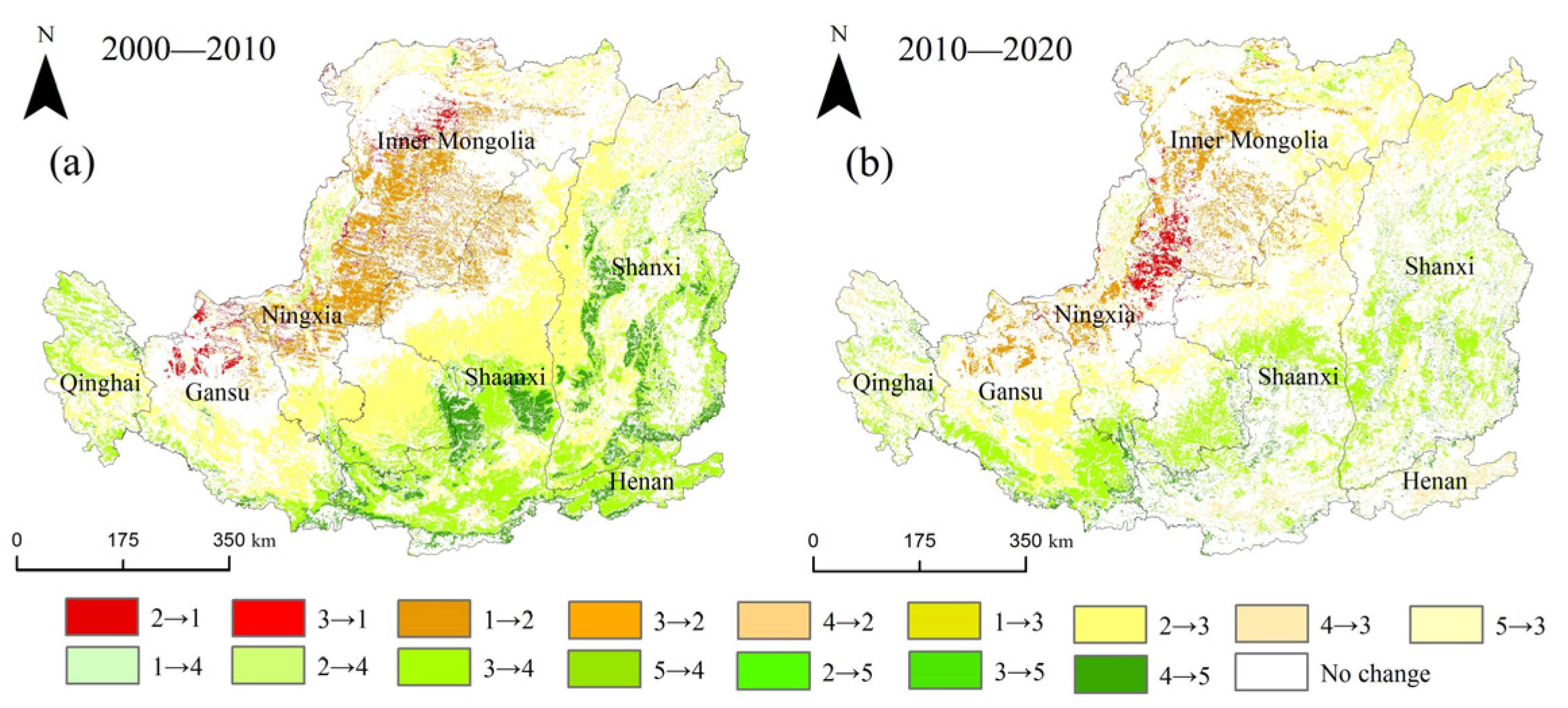
4.1.3. RSEI Transfer Analysis
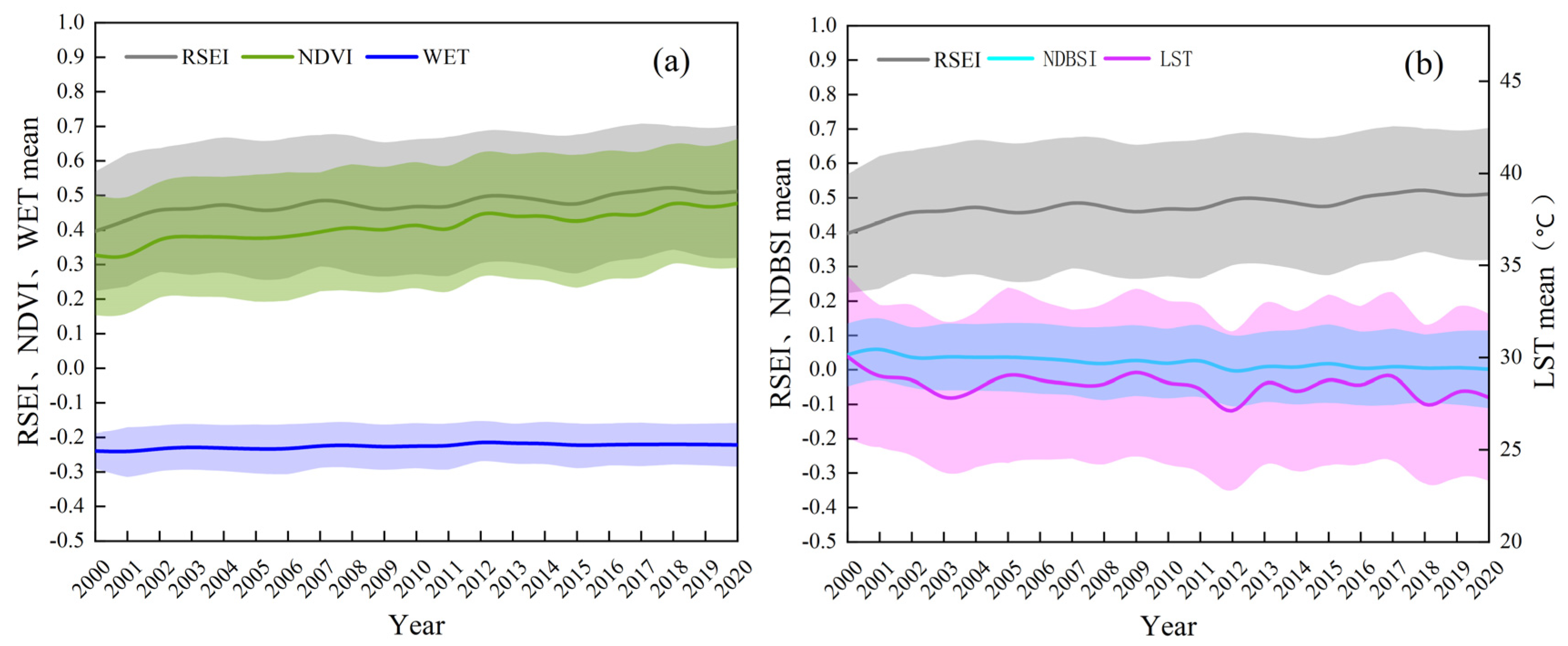
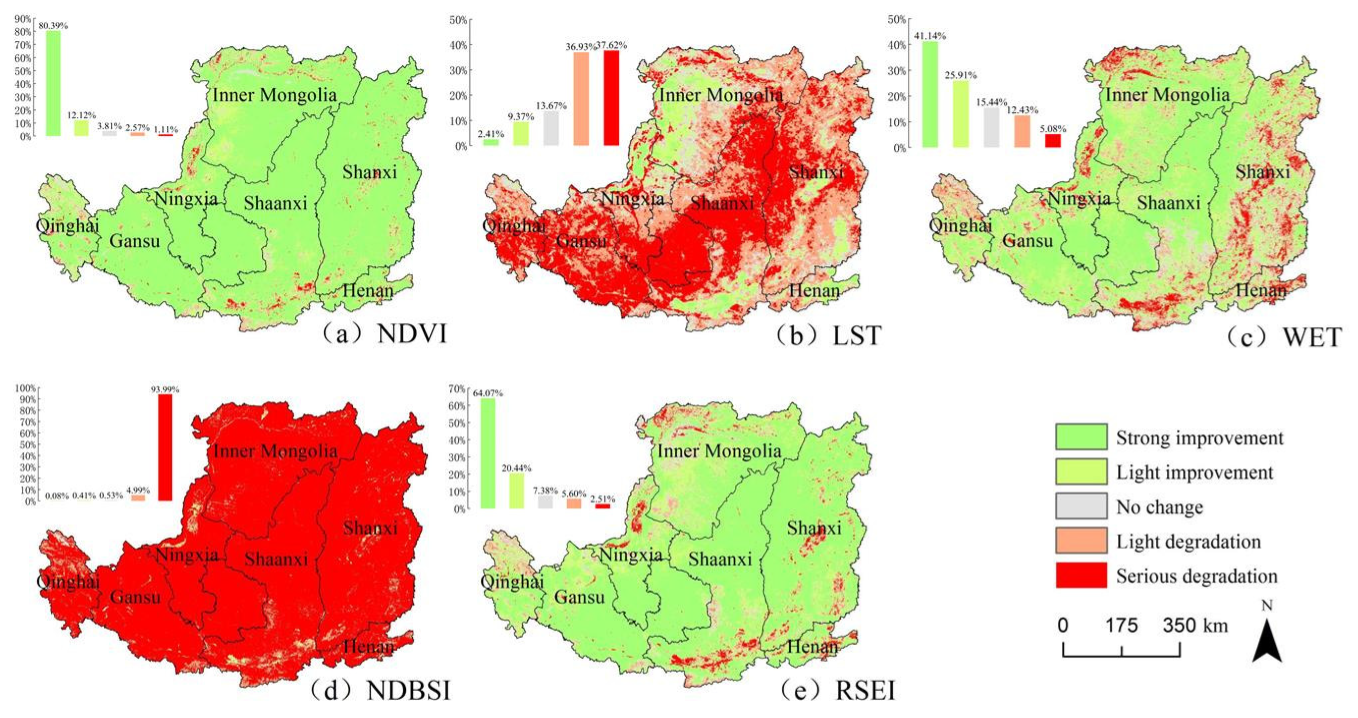
4.2. Trend Analysis of RSEI and Its Indicators in the LP
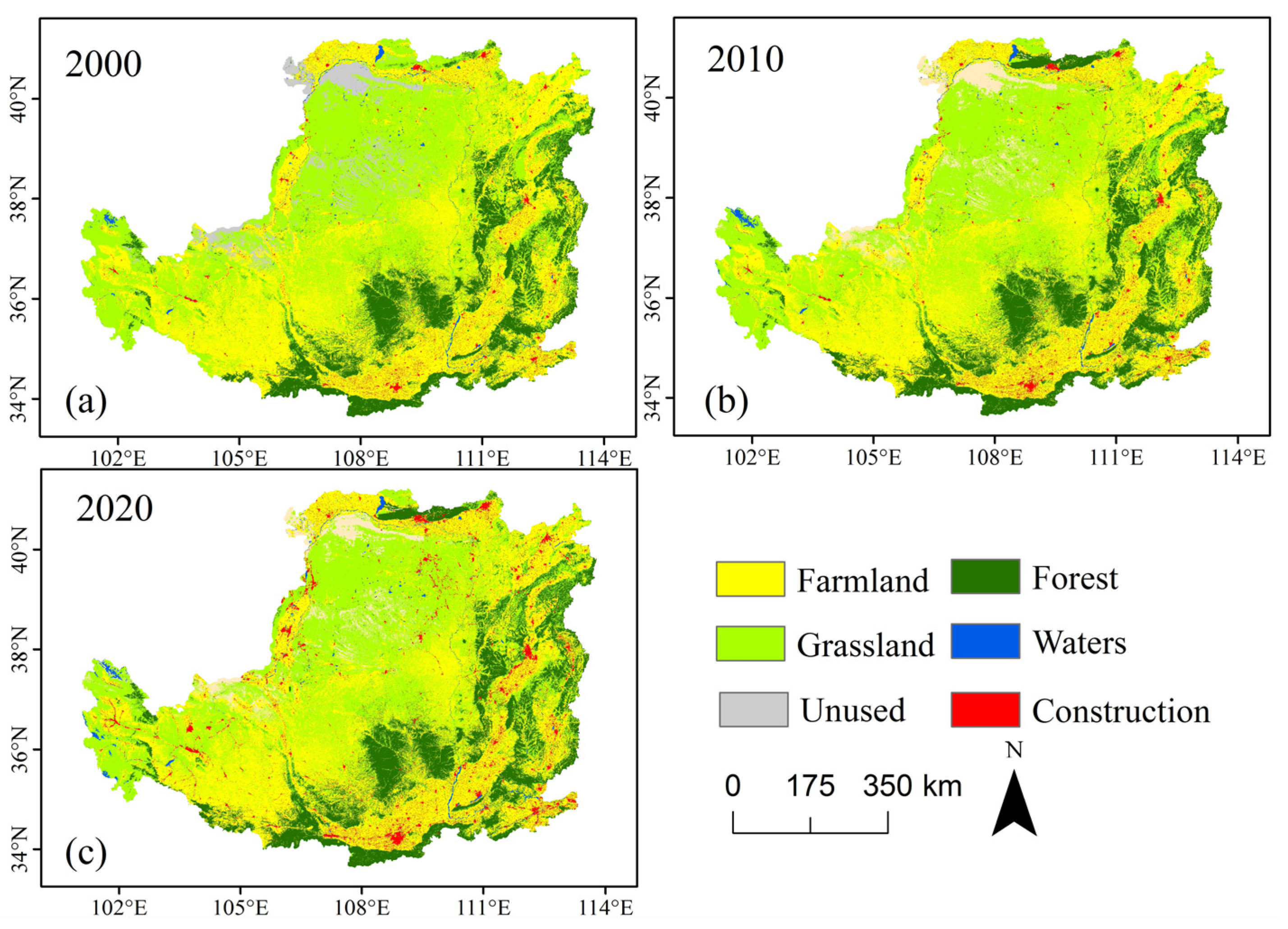
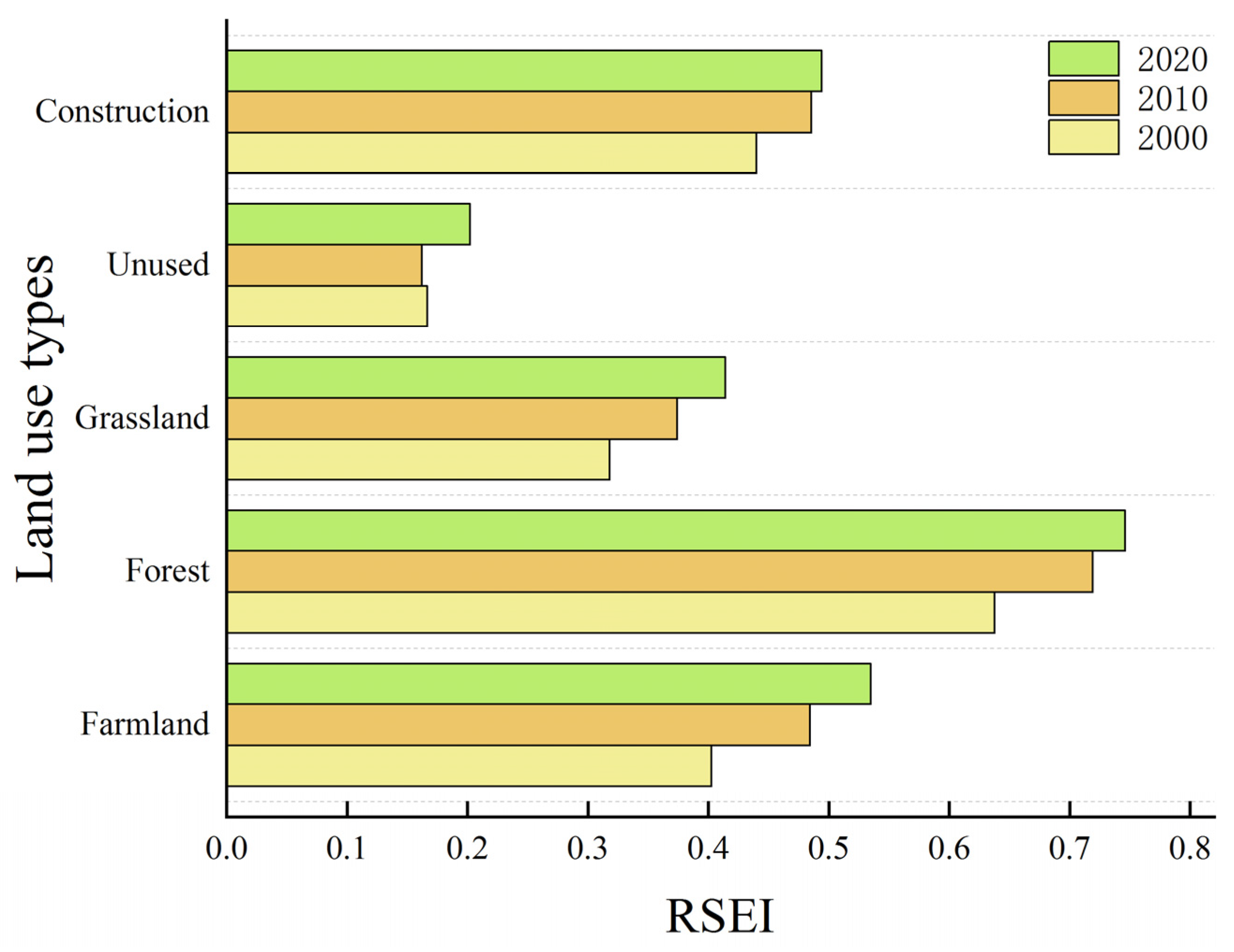
4.3. Relationship between Land Use Change and RSEI
4.4. Analysis of Driving Mechanism of RSEI
4.4.1. Single-Factor Detection Results
4.4.2. Multi-Factor Detection Results
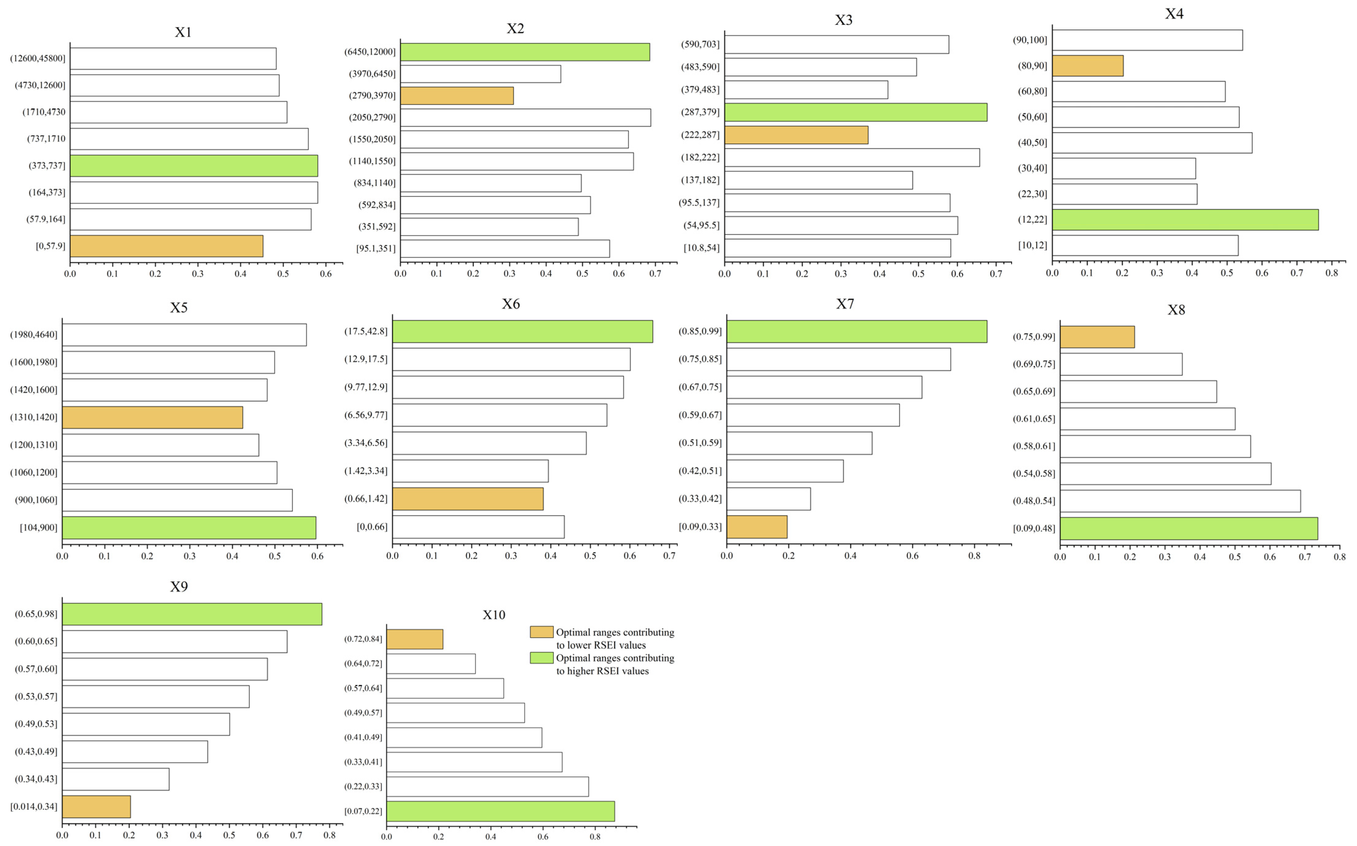
4.4.3. Optimal Ranges and Tipping Points of Factors Influencing RSEI
5. Discussion
5.1. Process of Ecological Restoration in the LP
5.2. Major Drivers of RSEI
5.3. Limitations and Future Work
6. Conclusions
Author Contributions
Funding
Institutional Review Board Statement
Informed Consent Statement
Data Availability Statement
Acknowledgments
Conflicts of Interest
References
- Ji, J.; Wang, S.; Zhou, Y.; Liu, W.; Wang, L. Spatiotemporal Change and Landscape Pattern Variation of Eco-Environmental Quality in Jing-Jin-Ji Urban Agglomeration From 2001 to 2015. IEEE Access 2020, 8, 125534–125548. [Google Scholar] [CrossRef]
- Ji, J.; Tang, Z.; Zhang, W.; Liu, W.; Jin, B.; Xi, X.; Wang, F.; Zhang, R.; Guo, B.; Xu, Z.; et al. Spatiotemporal and Multiscale Analysis of the Coupling Coordination Degree between Economic Development Equality and Eco-Environmental Quality in China from 2001 to 2020. Remote Sens. 2022, 14, 737. [Google Scholar] [CrossRef]
- Xu, H.; Wang, Y.; Guan, H.; Shi, T.; Hu, X. Detecting Ecological Changes with a Remote Sensing Based Ecological Index (RSEI) Produced Time Series and Change Vector Analysis. Remote Sens. 2019, 11, 2345. [Google Scholar] [CrossRef]
- An, M.; Xie, P.; He, W.; Wang, B.; Huang, J.; Khanal, R. Spatiotemporal change of ecologic environment quality and human interaction factors in three gorges ecologic economic corridor, based on RSEI. Ecol. Indic. 2022, 141, 109090. [Google Scholar] [CrossRef]
- Yurui, L.; Xuanchang, Z.; Zhi, C.; Zhengjia, L.; Zhi, L.; Yansui, L. Towards the progress of ecological restoration and economic development in China’s Loess Plateau and strategy for more sustainable development. Sci. Total Environ. 2021, 756, 143676. [Google Scholar] [CrossRef] [PubMed]
- Uchida, E.; Xu, J.; Rozelle, S. Grain for Green: Cost-Effectiveness and Sustainability of China’s Conservation Set-Aside Program. Land. Econ. 2005, 81, 247–264. [Google Scholar] [CrossRef]
- Chen, H.; Fleskens, L.; Schild, J.; Moolenaar, S.; Wang, F.; Ritsema, C. Impacts of large-scale landscape restoration on spatio-temporal dynamics of ecosystem services in the Chinese Loess Plateau. Landsc. Ecol. 2022, 37, 329–346. [Google Scholar] [CrossRef]
- Su, K.; Liu, H.; Wang, H. Spatial-Temporal Changes and Driving Force Analysis of Ecosystems in the Loess Plateau Ecological Screen. Forests 2022, 13, 54. [Google Scholar] [CrossRef]
- Frazier, A.E.; Bryan, B.A.; Buyantuev, A.; Chen, L.; Echeverria, C.; Jia, P.; Liu, L.; Li, Q.; Ouyang, Z.; Wu, J.; et al. Ecological civilization: Perspectives from landscape ecology and landscape sustainability science. Landsc. Ecol. 2019, 34, 1–8. [Google Scholar] [CrossRef]
- Wu, Z.; Dai, X.; Li, B.; Hou, Y. Livelihood consequences of the Grain for Green Programme across regional and household scales: A case study in the Loess Plateau. Land Use Policy 2021, 111, 105746. [Google Scholar] [CrossRef]
- Wang, S.; Peng, J.; Zhuang, J.; Kang, C.; Jia, Z. Underlying mechanisms of the geohazards of macro Loess discontinuities on the Chinese Loess Plateau. Eng. Geol. 2019, 263, 105357. [Google Scholar] [CrossRef]
- Li, P.; Chen, J.; Zhao, G.; Holden, J.; Liu, B.; Chan, F.K.S.; Hu, J.; Wu, P.; Mu, X. Determining the drivers and rates of soil erosion on the Loess Plateau since 1901. Sci. Total Environ. 2022, 823, 153674. [Google Scholar] [CrossRef] [PubMed]
- Jiang, H.; Fan, G.; Zhang, D.; Fan, Y. Evaluation of Eco-environmental Quality of Coal Mining Area Using Multi-source Data. Sci. Rep. 2022, 12, 6623. [Google Scholar] [CrossRef]
- Kasischke, E.S.; French, N.H.F.; Harrell, P.; Christensen, N.L.; Ustin, S.L.; Barry, D. Monitoring of wildfires in Boreal Forests using large area AVHRR NDVI composite image data. Sci. Total Environ. 1993, 45, 61–71. [Google Scholar] [CrossRef]
- Nagler, P.L.; Scott, R.L.; Westenburg, C.; Cleverly, J.R.; Glenn, E.P.; Huete, A.R. Evapotranspiration on western U.S. rivers estimated using the Enhanced Vegetation Index from MODIS and data from eddy covariance and Bowen ratio flux towers. Remote Sens. Environ. 2005, 97, 337–351. [Google Scholar] [CrossRef]
- Dousset, B.; Gourmelon, F. Satellite multi-sensor data analysis of urban surface temperatures and landcover. ISPRS J. Photogramm. Remote Sens. 2003, 58, 43–54. [Google Scholar] [CrossRef]
- Zheng, Z.; Wu, Z.; Chen, Y.; Guo, C.; Marinello, F. Instability of remote sensing based ecological index (RSEI) and its improvement for time series analysis. Sci. Total Environ. 2022, 814, 152595. [Google Scholar] [CrossRef]
- Becker, F.; Choudhury, B.J. Relative sensitivity of normalized difference vegetation Index (NDVI) and microwave polarization difference Index (MPDI) for vegetation and desertification monitoring. Remote Sens. Environ. 1988, 24, 297–311. [Google Scholar] [CrossRef]
- Khan, J.; Wang, P.; Xie, Y.; Wang, L.; Li, L. Mapping MODIS LST NDVI Imagery for Drought Monitoring in Punjab Pakistan. IEEE Access 2018, 6, 19898–19911. [Google Scholar] [CrossRef]
- Chang, Y.; Hou, K.; Wu, Y.; Li, X.; Zhang, J. A conceptual framework for establishing the index system of ecological environment evaluation-A case study of the upper Hanjiang River, China. Ecol. Indic. 2019, 107, 105568. [Google Scholar] [CrossRef]
- Xu, H. A remote sensing urban ecological index and its application. Acta Ecol. Sin. 2013, 33, 7853–7862. (In Chinese) [Google Scholar]
- Zou, Z.-h.; Yun, Y.; Sun, J.-n. Entropy method for determination of weight of evaluating indicators in fuzzy synthetic evaluation for water quality assessment. J. Environ. 2006, 18, 1020–1023. [Google Scholar] [CrossRef]
- Saaty, T.L. A scaling method for priorities in hierarchical structures. J. Math. Psychol. 1977, 15, 234–281. [Google Scholar] [CrossRef]
- Liu, B.; Zhang, F.; Wan, W.; Luo, X. Multi-objective Decision-Making for the Ecological Operation of Built Reservoirs Based on the Improved Comprehensive Fuzzy Evaluation Method. Water Resour. Manag. 2019, 33, 3949–3964. [Google Scholar] [CrossRef]
- Dinh, T.C.; Dinh, T.C.; Anh, T.T.; Xuan, B.M.; Manh, L.N.; Van Thanh, D.; Le Van, D.; Thanh, H.D.; Quang, T.N. Mapping Seismic Zones Based on the Geomorphic Indices and the Analytic Hierarchy Process (AHP): A Case Study in Cao Bang Province and Adjacent Areas (Vietnam). J. Geol. Soc. India 2021, 97, 1565–1573. [Google Scholar] [CrossRef]
- Maity, S.; Das, S.; Pattanayak, J.M.; Bera, B.; Shit, P.K. Assessment of ecological environment quality in Kolkata urban agglomeration, India. Urban Ecosyst. 2022, 25, 1137–1154. [Google Scholar] [CrossRef]
- Qureshi, S.; Alavipanah, S.K.; Konyushkova, M.; Mijani, N.; Fathololomi, S.; Firozjaei, M.K.; Homaee, M.; Hamzeh, S.; Kakroodi, A.A. A Remotely Sensed Assessment of Surface Ecological Change over the Gomishan Wetland, Iran. Remote Sens. 2020, 12, 2898. [Google Scholar] [CrossRef]
- Gorelick, N.; Hancher, M.; Dixon, M.; Ilyushchenko, S.; Thau, D.; Moore, R. Google Earth Engine: Planetary-scale geospatial analysis for everyone. Remote Sens. Environ. 2017, 202, 18–27. [Google Scholar] [CrossRef]
- Yang, X.; Meng, F.; Fu, P.; Zhang, Y.; Liu, Y. Spatiotemporal change and driving factors of the Eco-Environment quality in the Yangtze River Basin from 2001 to 2019. Ecol. Indic. 2021, 131, 108214. [Google Scholar] [CrossRef]
- Sen, P.K. Estimates of the Regression Coefficient Based on Kendall’s Tau. J. Am. Stat. Assoc. 1968, 63, 1379–1389. [Google Scholar] [CrossRef]
- Kendall, M.G. Rank Correlation Methods; Springer: Boston, MA, USA, 1948. [Google Scholar]
- Mann, H.B. Nonparametric Tests Against Trend. Econometrica 1945, 13, 245. [Google Scholar] [CrossRef]
- Yin, S. Decadal trends of MERRA-estimated PM2.5 concentrations in East Asia and potential exposure from 1990 to 2019. Atmos. Environ. 2021, 264, 118690. [Google Scholar] [CrossRef]
- Ruiz-Alvarez, O.; Singh, V.P.; Enciso-Medina, J.; Ontiveros-Capurata, R.E.; Corrales-Suastegui, A. Spatio-Temporal Trends of Monthly and Annual Precipitation in Aguascalientes, Mexico. Atmosphere 2020, 11, 437. [Google Scholar] [CrossRef]
- Lü, Y.; Fu, B.; Feng, X.; Zeng, Y.; Liu, Y.; Chang, R.; Sun, G.; Wu, B. A policy-driven large scale ecological restoration: Quantifying ecosystem services changes in the Loess Plateau of China. PLoS ONE 2012, 7, e31782. [Google Scholar] [CrossRef]
- Xiao, Y.; Wang, R.; Wang, F.; Huang, H.; Wang, J. Investigation on spatial and temporal variation of coupling coordination between socioeconomic and ecological environment: A case study of the Loess Plateau, China. Ecol. Indic. 2022, 136, 108667. [Google Scholar] [CrossRef]
- Song, Y.; Xue, D.; Dai, L.; Wang, P.; Huang, X.; Xia, S. Land cover change and eco-environmental quality response of different geomorphic units on the Chinese Loess Plateau. J. Arid Land. 2020, 12, 29–43. [Google Scholar] [CrossRef]
- Huete, A.; Didan, K.; Miura, T.; Rodriguez, E.P.; Gao, X.; Ferreira, L.G. Overview of the radiometric and biophysical performance of the MODIS vegetation indices. Remote Sens. Environ. 2002, 83, 195–213. [Google Scholar] [CrossRef]
- Airiken, M.; Zhang, F.; Chan, N.W.; Kung, H.T. Assessment of spatial and temporal ecological environment quality under land use change of urban agglomeration in the North Slope of Tianshan, China. Environ. Sci. Pollut. Res. Int. 2022, 29, 12282–12299. [Google Scholar] [CrossRef]
- Lobser, S.; Cohen, W. MODIS tasselled cap: Land cover characteristics expressed through transformed MODIS data. Int. J. Remote Sens. 2007, 28, 5079–5101. [Google Scholar] [CrossRef]
- Zhang, X.Y.; Schaaf, C.B.; Friedl, M.A.; Strahler, A.H.; Gao, F.; Hodges, J.C.F. MODIS tasseled cap transformation and its utility. In Proceedings of the IEEE International Geoscience and Remote Sensing Symposium, Toronto, ON, Canada, 24–28 June 2002; IEEE: Piscataway, NJ, USA, 2002; Volume 2, pp. 1063–1065. [Google Scholar]
- Xu, H. A new index for delineating built-up land features in satellite imagery. Int. J. Remote Sens. 2008, 29, 4269–4276. [Google Scholar] [CrossRef]
- Rikimaru, A.; Roy, P.S.; Miyatake, S. Tropical forest cover density mapping. Trop Ecol. 2002, 43, 39–47. [Google Scholar]
- Wang, J.; Xu, C. Geodetector: Principle and prospective. Acta Geogr. Sin. 2017, 72, 116–134. [Google Scholar]
- Li, Y.; Zhang, G.; Lin, T.; Ye, H.; Liu, Y.; Chen, T.; Liu, W. The spatiotemporal changes of remote sensing ecological index in towns and the influencing factors: A case study of Jizhou District, Tianjin. Acta Ecol. Sin. 2022, 42, 474–486. [Google Scholar]
- Zhang, Q.-J.; Fu, B.-J.; Chen, L.-D.; Zhao, W.-W.; Yang, Q.-K.; Liu, G.-B.; Gulinck, H. Dynamics and driving factors of agricultural landscape in the semiarid hilly area of the Loess Plateau, China. Agric. Ecosyst. Environ. 2004, 103, 535–543. [Google Scholar] [CrossRef]
- Sun, W.; Song, X.; Mu, X.; Gao, P.; Wang, F.; Zhao, G. Spatiotemporal vegetation cover variations associated with climate change and ecological restoration in the Loess Plateau. Agric. For. Meteorol. 2015, 209–210, 87–99. [Google Scholar] [CrossRef]
- Naeem, S.; Zhang, Y.; Zhang, X.; Tian, J.; Abbas, S.; Luo, L.; Meresa, H.K. Both climate and socioeconomic drivers contribute to vegetation greening of the Loess Plateau. Sci. Bull. 2021, 66, 1160–1163. [Google Scholar] [CrossRef]
- Yuan, B.; Fu, L.; Zou, Y.; Zhang, S.; Chen, X.; Li, F.; Deng, Z.; Xie, Y. Spatiotemporal change detection of ecological quality and the associated affecting factors in Dongting Lake Basin, based on RSEI. J. Clean. Prod. 2021, 302, 126995. [Google Scholar] [CrossRef]
- Xia, Q.-Q.; Chen, Y.-N.; Zhang, X.-Q.; Ding, J.-L. Spatiotemporal Changes in Ecological Quality and Its Associated Driving Factors in Central Asia. Remote Sens. 2022, 14, 3500. [Google Scholar] [CrossRef]
- Liu, C.; Li, W.; Zhu, G.; Zhou, H.; Yan, H.; Xue, P. Land Use/Land Cover Changes and Their Driving Factors in the Northeastern Tibetan Plateau Based on Geographical Detectors and Google Earth Engine: A Case Study in Gannan Prefecture. Remote Sens. 2020, 12, 3139. [Google Scholar] [CrossRef]
- Ariken, M.; Zhang, F.; Liu, K.; Fang, C.; Kung, H.-T. Coupling coordination analysis of urbanization and eco-environment in Yanqi Basin based on multi-source remote sensing data. Ecol. Indic. 2020, 114, 106331. [Google Scholar] [CrossRef]
- Su, C.; Fu, B. Evolution of ecosystem services in the Chinese Loess Plateau under climatic and land use changes. Glob. Planet Chang. 2013, 101, 119–128. [Google Scholar] [CrossRef]
- Ren, Y.; Lü, Y.; Fu, B.; Comber, A.; Li, T.; Hu, J. Driving Factors of Land Change in China’s Loess Plateau: Quantification Using Geographically Weighted Regression and Management Implications. Remote Sens. 2020, 12, 453. [Google Scholar] [CrossRef]
- Liu, G. Soil Conservation and Sustainable Agriculture on the Loess Plateau: Challenges and Prospects. Ambio 1999, 28, 663–668. [Google Scholar]
- Deng, X.-P.; Shan, L.; Zhang, H.; Turner, N.C. Improving agricultural water use efficiency in arid and semiarid areas of China. Agric. Water Manag. 2006, 80, 23–40. [Google Scholar] [CrossRef]
- Bullock, A.; King, B. Evaluating China’s Slope Land Conversion Program as sustainable management in Tianquan and Wuqi Counties. J. Environ. Manag. 2011, 92, 1916–1922. [Google Scholar] [CrossRef]
- Li, Z.; Yang, L.; Wang, G.; Hou, J.; Xin, Z.; Liu, G.; Fu, B. The management of soil and water conservation in the Loess Plateau of China: Present situations, problems, and counter-solutions. Acta Ecol. Sin. 2019, 39, 7398–7409. [Google Scholar]
- Du, X.; Zhao, X.; Liang, S.; Zhao, J.; Xu, P.; Wu, D. Quantitatively Assessing and Attributing Land Use and Land Cover Changes on China’s Loess Plateau. Remote Sens. 2020, 12, 353. [Google Scholar] [CrossRef]
- Ping, Z.; Anbang, W.; Xinbao, Z.; Xiubin, H. Soil conservation and sustainable eco-environment in the Loess Plateau of China. Environ. Earth Sci. 2013, 68, 633–639. [Google Scholar] [CrossRef]
- Venkatesh, K.; John, R.; Chen, J.; Xiao, J.; Amirkhiz, R.G.; Giannico, V.; Kussainova, M. Optimal ranges of social-environmental drivers and their impacts on vegetation dynamics in Kazakhstan. Sci. Total Environ. 2022, 847, 157562. [Google Scholar] [CrossRef]
- Zhang, Y.; Jiang, X.; Lei, Y.; Gao, S. The contributions of natural and anthropogenic factors to NDVI variations on the Loess Plateau in China during 2000–2020. Ecol. Indic. 2022, 143, 109342. [Google Scholar] [CrossRef]
- Mehri, A.; Salmanmahiny, A.; Tabrizi, A.R.M.; Mirkarimi, S.H.; Sadoddin, A. Investigation of likely effects of land use planning on reduction of soil erosion rate in river basins: Case study of the Gharesoo River Basin. Catena 2018, 167, 116–129. [Google Scholar] [CrossRef]
- Kumar, R.; Nath, A.J.; Nath, A.; Sahu, N.; Pandey, R. Landsat-based multi-decadal spatio-temporal assessment of the vegetation greening and browning trend in the Eastern Indian Himalayan Region. Remote Sens. Appl. Soc. Environ. 2022, 25, 100695. [Google Scholar] [CrossRef]
- Wang, X.; Wu, J.; Liu, Y.; Hai, X.; Shanguan, Z.; Deng, L. Driving factors of ecosystem services and their spatiotemporal change assessment based on land use types in the Loess Plateau. J. Environ. Manag. 2022, 311, 114835. [Google Scholar] [CrossRef] [PubMed]
- Beyaztas, U.; Salih, S.Q.; Chau, K.-W.; Al-Ansari, N.; Yaseen, Z.M. Construction of functional data analysis modeling strategy for global solar radiation prediction: Application of cross-station paradigm. Eng. Appl. Comp. Fluid 2019, 13, 1165–1181. [Google Scholar] [CrossRef]


| Indicators | Product | Spatial Resolution (m) | Temporal Resolution (d) | Number of Scenes | Data Level | Years |
|---|---|---|---|---|---|---|
| NDVI | MOD13A1 | 500 | 16 | 30 | L3 | 2000, 2010, 2020 |
| LST | MOD11A2 | 1000 | 8 | 61 | L3 | 2000, 2010, 2020 |
| WET/NDBSI | MOD09A1 | 500 | 8 | 61 | L2 | 2000, 2010, 2020 |
| Factor Types | Driving Factors | Factor Symbols | Unit | Type Numbers |
|---|---|---|---|---|
| Socioeconomic factors | Population density | X1 | people/ | 8 |
| Gross domestic product (GDP) | X2 | Hundred million yuan | 10 | |
| Gross output value of farming, forest, animal husbandry and fishery | X3 | Hundred million yuan | 10 | |
| Natural Factors | Land use types | X4 | — | 9 |
| Elevation | X5 | m | 8 | |
| Slope | X6 | ° | 8 | |
| Model factors | NDVI | X7 | — | 8 |
| LST | X8 | — | 8 | |
| WET | X9 | — | 8 | |
| NDBSI | X10 | — | 8 |
| Year | Indicators | PC1 | PC2 | PC3 | PC4 |
|---|---|---|---|---|---|
| 2000 | NDVI | 0.6274 | 0.4617 | 0.4051 | −0.4785 |
| LST | −0.3535 | −0.4160 | 0.8203 | −0.1703 | |
| WET | 0.4513 | −0.7636 | −0.2704 | −0.3740 | |
| NDBSI | −0.5269 | 0.1747 | −0.2996 | −0.7759 | |
| Eigenvalue | 0.0691 | 0.0053 | 0.0040 | 0.0012 | |
| Percent eigenvalue (%) | 86.8091 | 6.6583 | 5.0251 | 1.5075 | |
| 2010 | NDVI | 0.5772 | 0.4744 | −0.3917 | −0.5368 |
| LST | −0.3362 | 0.7206 | 0.5867 | −0.1528 | |
| WET | 0.4248 | −0.4377 | 0.6717 | −0.4203 | |
| NDBSI | −0.6109 | −0.2527 | −0.2259 | −0.7154 | |
| Eigenvalue | 0.0866 | 0.0048 | 0.0042 | 0.0016 | |
| Percent eigenvalue (%) | 89.0947 | 4.9383 | 4.3210 | 1.6461 | |
| 2020 | NDVI | 0.6089 | 0.1932 | 0.5865 | −0.4977 |
| LST | −0.3496 | 0.9141 | −0.0931 | −0.1826 | |
| WET | 0.4286 | −0.0013 | −0.8003 | −0.4191 | |
| NDBSI | −0.5684 | −0.3563 | 0.0820 | −0.7370 | |
| Eigenvalue | 0.0782 | 0.0054 | 0.0042 | 0.0015 | |
| Percent eigenvalue (%) | 87.5700 | 6.0470 | 4.7032 | 1.6797 |
| Land Use Types | Proportion of the Corresponding Area | ||
|---|---|---|---|
| 2000 | 2010 | 2020 | |
| Farmland | 40.02% | 39.33% | 38.95% |
| Forest | 15.45% | 16.61% | 16.90% |
| Grassland | 38.04% | 37.04% | 35.45% |
| Waters | 0.69% | 0.76% | 0.91% |
| Unused | 3.93% | 3.89% | 3.65% |
| Construction | 1.87% | 2.37% | 4.14% |
| Year | Socioeconomic Factors | Natural Factors | Model Factors | ||||||||
|---|---|---|---|---|---|---|---|---|---|---|---|
| Factors | X1 | X2 | X3 | X4 | X5 | X6 | X7 | X8 | X9 | X10 | |
| 2000 | q | 0.0108 | 0.0947 | 0.1284 | 0.2447 | 0.0880 | 0.1718 | 0.7990 | 0.6366 | 0.7288 | 0.7987 |
| p | 0.000 | 0.000 | 0.000 | 0.000 | 0.000 | 0.000 | 0.000 | 0.000 | 0.000 | 0.000 | |
| 2010 | q | 0.0150 | 0.2654 | 0.1288 | 0.2855 | 0.0807 | 0.2011 | 0.8188 | 0.6559 | 0.7637 | 0.8477 |
| p | 0.000 | 0.000 | 0.000 | 0.000 | 0.000 | 0.000 | 0.000 | 0.000 | 0.000 | 0.000 | |
| 2020 | q | 0.0175 | 0.3161 | 0.1366 | 0.2937 | 0.0642 | 0.2420 | 0.8279 | 0.6356 | 0.7596 | 0.8357 |
| p | 0.000 | 0.000 | 0.000 | 0.000 | 0.000 | 0.000 | 0.000 | 0.000 | 0.000 | 0.000 | |
Publisher’s Note: MDPI stays neutral with regard to jurisdictional claims in published maps and institutional affiliations. |
© 2022 by the authors. Licensee MDPI, Basel, Switzerland. This article is an open access article distributed under the terms and conditions of the Creative Commons Attribution (CC BY) license (https://creativecommons.org/licenses/by/4.0/).
Share and Cite
Zhang, J.; Yang, G.; Yang, L.; Li, Z.; Gao, M.; Yu, C.; Gong, E.; Long, H.; Hu, H. Dynamic Monitoring of Environmental Quality in the Loess Plateau from 2000 to 2020 Using the Google Earth Engine Platform and the Remote Sensing Ecological Index. Remote Sens. 2022, 14, 5094. https://doi.org/10.3390/rs14205094
Zhang J, Yang G, Yang L, Li Z, Gao M, Yu C, Gong E, Long H, Hu H. Dynamic Monitoring of Environmental Quality in the Loess Plateau from 2000 to 2020 Using the Google Earth Engine Platform and the Remote Sensing Ecological Index. Remote Sensing. 2022; 14(20):5094. https://doi.org/10.3390/rs14205094
Chicago/Turabian StyleZhang, Jing, Guijun Yang, Liping Yang, Zhenhong Li, Meiling Gao, Chen Yu, Enjun Gong, Huiling Long, and Haitang Hu. 2022. "Dynamic Monitoring of Environmental Quality in the Loess Plateau from 2000 to 2020 Using the Google Earth Engine Platform and the Remote Sensing Ecological Index" Remote Sensing 14, no. 20: 5094. https://doi.org/10.3390/rs14205094
APA StyleZhang, J., Yang, G., Yang, L., Li, Z., Gao, M., Yu, C., Gong, E., Long, H., & Hu, H. (2022). Dynamic Monitoring of Environmental Quality in the Loess Plateau from 2000 to 2020 Using the Google Earth Engine Platform and the Remote Sensing Ecological Index. Remote Sensing, 14(20), 5094. https://doi.org/10.3390/rs14205094