Article

Modeling the Leaf Area Index of Inner Mongolia Grassland Based on Machine Learning Regression Algorithms Incorporating Empirical Knowledge

1
Institute of Agricultural Resources and Regional Planning, Chinese Academy of Agricultural Sciences, Beijing 100081, China
2
College of Environmental and Resource Sciences, Zhejiang University, Hangzhou 310058, China
3
Natural Resources Comprehensive Survey Command Center, China Geological Survey, Beijing 100055, China
4
Jiangsu Key Laboratory of Crop Genetics and Physiology, Jiangsu Key Laboratory of Crop Cultivation and Physiology, Agricultural College, Yangzhou University, Yangzhou 225009, China
5
EcoGIS Center, Tashkent Institute of Irrigation and Agricultural Mechanization Engineers (TIIAME), Tashkent 100000, Uzbekistan
6
Department of Environmental and Earth Science, American University of Central Asia, Bishkek 720060, Kyrgyzstan
7
Department of Geography, Environment, and Spatial Sciences, Michigan State University, East Lansing, MI 48824, USA
8
Earth and Environmental Sciences Department, University of Central Asia, Bishkek 720001, Kyrgyzstan
*
Author to whom correspondence should be addressed.
Remote Sens. 2022, 14(17), 4196; https://doi.org/10.3390/rs14174196
Submission received: 14 July 2022 / Revised: 21 August 2022 / Accepted: 22 August 2022 / Published: 26 August 2022
(This article belongs to the Special Issue Remote Sensing of Ecosystems)

Abstract

:
Leaf area index (LAI) is one of the key biophysical indicators for characterizing the growth and status of vegetation and is also used in modeling earth system processes. Machine learning algorithms (MLAs) such as random forest regression (RFR), artificial neural network regression (ANNR) and support vector regression (SVR) based on satellite data have been widely used for the estimation of LAI. However, the selection of input variables has a great impact on the estimation performance of MLAs. In this study, we aimed to improve the LAI inversion model of Inner Mongolia grassland based on MLAs incorporating empirical knowledge. Firstly, we used the ANNR, SVR and RFR approaches, respectively, to rank the input variables including vegetation indices, climate factors, soil factors and topography factors and found that Normalized Difference Phenology Index (NDPI) contributed the most to LAI estimation. Secondly, we selected four sets of input variables, namely, all variables—A, model selected variables—B, overlapping variables—C and self-defined variables—D, respectively. Subsequently, we built twelve LAI estimation models (RFR-A, RFR-B, RFR-C, etc.) based on three MLAs and four sets of input variables. The evaluation of them showed the RFR produced higher prediction accuracy, followed by ANNR and SVR. Furthermore, the RFR-D presented the highest accuracy in predicting LAI (R2 = 0.55, RMSE = 0.37 m2/m2, MAE = 0.29 m2/m2). Finally, we compared our results with MODIS LAI and GEOV2 LAI products and found that all of them showed a similar spatial distribution of grassland LAI in the four sub-regions covering all grassland types, but our model exhibited larger LAI values in the desert steppe and smaller LAI values in the others. These findings demonstrated that MLAs incorporating empirical knowledge could improve the accuracy of modelling LAI and further study is necessary to reduce the uncertainty in LAI mapping in grassland.

Graphical Abstract

1. Introduction

Grassland is a huge carbon stock with a strong carbon sink function [1]. It not only has an important position in the carbon cycle of terrestrial ecosystem, but also plays an important role in achieving the goals of carbon peaking and carbon neutrality. Leaf area index (LAI), defined as half leaf surface area per unit ground surface area, is a quantitative description of the amount of leaf area in an ecosystem [2,3,4]. As an important indicator for describing grassland growth and status, LAI is closely related to vegetation light use, evapotranspiration and energy exchange assessment. Meanwhile, LAI can indirectly reflect climate change, which serves as an important basis for vegetation feedback to the climate system [4,5,6,7,8]. The wide geographic distribution, complex grass species and high spatial heterogeneity of natural grassland make LAI inversion difficult [9,10]. In addition, direct validation of coarse satellite-derived products based on ground truth data is needed. One way to validate the LAI products from regional to global domains is to apply high-resolution LAI maps as a reference [11]. Therefore, it requires approaches to up-scale the ground truth data to the corresponding satellite products. These research implications highlight that the development of LAI inversion algorithms and related datasets with a high spatial resolution is necessary.
Traditional methods of measuring LAI rely heavily on ground-based measurements, which are time-consuming, complex and not easily carried out over long periods of time across large areas [12,13]. Since the 1980s, a variety of satellites carrying different optical sensors have been launched to provide continuous and repeated observations on the earth, which has brought a new era of LAI estimation [14]. With the availability of satellite data, it is possible to estimate the LAI and further analyze the spatial and temporal characteristics of the LAI on large scale and over long time series [15,16]. Various studies have assessed methods for quantitative LAI estimation using satellite data, which include parametric regression methods, nonparametric regression methods including linear and nonlinear machine learning algorithms (MLAs), physical model methods and hybrid model methods that combine RTM simulations with MLAs [17,18,19]. However, considering the global or regional monitoring applications, the statistical approaches based on vegetation indices (VIs) may be too simplistic while radiative transfer models may be too cumbersome to generate near real-time and accurate products [20].
As canopy characteristic inversion techniques, MLAs have shown impressive performances in their ability to map the non-linear relationship between the canopy parameterizes and the reflected signal, and in their fast-mapping speed compared to look-up tables [19,20,21,22]. With advances in computer technology and related techniques, the applications of MLAs cover broad areas, including vegetation, water resources and meteorology and have yielded encouraging results [23,24,25] Several studies have documented the successful application of MLAs to estimate LAI for various vegetation types, including crops [22], forests [24] and grassland [26]. Meanwhile, comparisons between random forest regression (RFR), support vector regression (SVR) and artificial neural networks regression (ANNR) have indicated that these methods have similar competitive performances [27,28]. Additional studies have shown that multi-factor models have advantages over single-factor models in simulating canopy parameters using MLAs [9,29]. Therefore, multiple factors affecting grassland LAI estimation, such as topography, climate, soil, and grass types should be taken into consideration in LAI modeling.
Previous studies have confirmed the effectiveness of applying MLAs to grassland LAI estimation. However, the datasets in these studies were collected within limited study areas and sample plots. Some of them focused on using the reflectance of waveband and VIs as input variables [26]. It is highly possible that there may be differences in the form and accuracy of LAI estimation models according to various datasets and different regions. Therefore, this study compares the performance of different MLAs in estimating LAI in combination with different sets of input variables using the same dataset collected from 191 in situ LAI sample plots, with the main objectives of (1) assessing the importance of multiple variables in the estimation of grassland LAI; (2) developing a high accuracy MLAs model incorporating empirical knowledge to predict LAI; and (3) analyzing the similarities and differences between our results and major satellite-based LAI products.

2. Materials and Methods
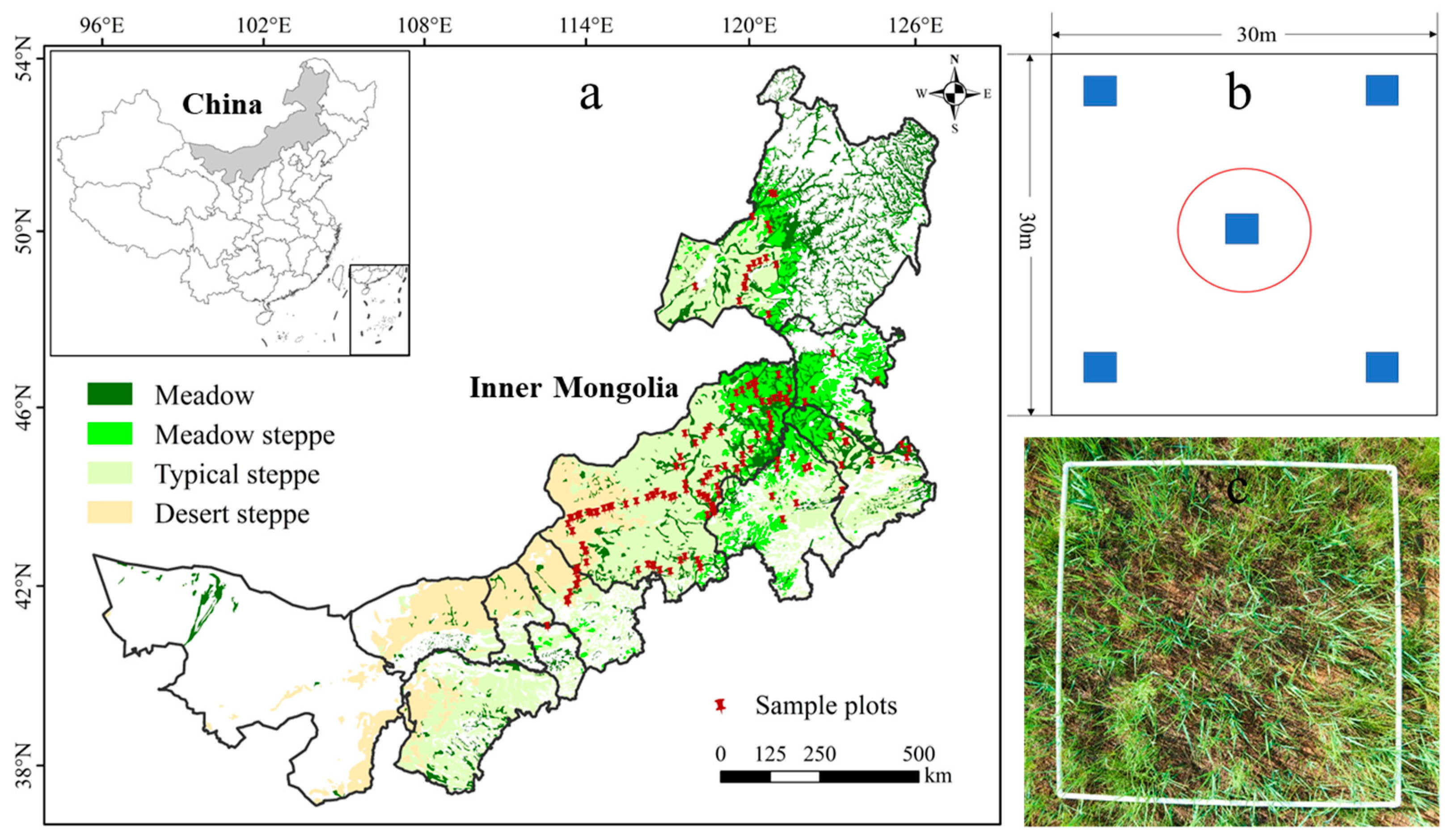
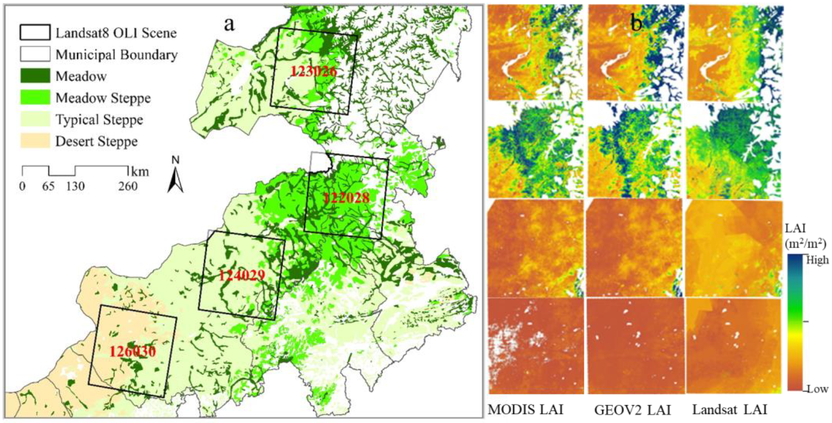
2.1. Study Region

The Inner Mongolia steppe (97°12′~126°04′E, 37°34′~53°23′N) is an important part of the Eurasia grassland, located in an arid and semi-arid region at mid-latitude, with a typical temperate continental climate. The average annual temperature ranges from 0 to 8 °C and the annual total precipitation ranges from 50 to 450 mm. From northeast to southwest, precipitation gradually decreases, and temperature gradually increases, creating a zonal distribution of soil and vegetation. The horizontal zonation of the Inner Mongolia steppe is relatively obvious, transitioning from meadow steppe and typical steppe to desert steppe. The meadow steppe is rich in species, with a magnificent appearance and high productivity; the typical steppe is the most representative type of temperate steppe with a medium coverage and productivity; the desert steppe is short and sparse, with the lowest coverage and productivity (Figure 1a).

2.2. Data Collection and Processing

2.2.1. In Situ LAI Measurement

We obtained a total of 191 in situ LAI sample plots through field surveys from July to August during the peak grassland growth in the year of 2015, 2016, 2018 and 2019 (Figure 1a). In each 30 m × 30 m sample plot, five 1 × 1 m quadratic subplots (one in the center and four in each corner) were established (Figure 1b,c). A handheld Garmin GPS 72H was used to determine the geographic location of each sample plot in the field. The LAI was measured with a LAI-2200C plant canopy analyzer (Li-Cor, Lincoln, NE, USA) at a 270° view cap. In each subplot, the LAI value was obtained according to the “ABBBBB” principle, where the A represented the reading value above the canopy and the B represented the reading value below the canopy. The measurements were collected under suitable sky conditions, near sunrise or sunset or on cloudy days. The LAI value of each sample plot was acquired by averaging the measurements of the five subplots.

2.2.2. Remotely Sensed Data

We used Landsat8 OLI (Operational Land Imager) dataset in this study. The spectral bands of Landsat8 OLI provided by the USGS (United States Geological Survey) shared data platform include visible (452–512, 532–590, 636–673 nm), near-infrared (NIR; 851–879 nm) and shortwave infrared (SWIR; 1566–1651, 2107–2294 nm) wavelengths (Figure 2b), with a spatial resolution of 30 m and 16-day return cycle. The spatial resolution of 30 m is higher than that of existing LAI products and better reflects differences between regions. It is available from the GEE (Google Earth Engine) platform, which is named as “USGS Landsat8 Level 2, Collection 2, Tier 1”. The good quality surface reflectance data at each wavelength band were used to calculate VIs subsequently. The VIs included RVI, NDVI, TDVI, CI and NDPI (Table 1).
The MODIS LAI and GEOV2 LAI are two global LAI products that are widely used in the research community. The MODIS LAI product (MOD15A2H) is provided in the sinusoidal projection at an 8-day temporal resolution and a 500 m spatial resolution. The MODIS LAI retrieval algorithm includes a primary algorithm based on a three-dimensional (3D) radiative transfer model and an alternate algorithm for regression relations [35]. The algorithm chooses the “best” pixel available from all the acquisitions of the Terra sensor from within the 8-day time step. The dataset ranges from 2000 to the present (https://ladswed.nascom.nasa.gov/, accessed on 12 October 2020). The GEOV2 LAI product is provided in the Plate Carrée projection at a 10-day temporal resolution and a 1 km spatial resolution. It is derived from the SPOT/VEGETATION sensor data based on a neural network. Frist, they obtain a training dataset, which is a fused LAI using the CYCLOPE and MODIS LAI products, and then the calibrated neural network is used to obtain the GEOV2 LAI product [36]. The dataset ranges from 1999 to the present (http://land.copernicus.eu/global/, accessed on 12 October 2020).

2.2.3. Climate, Soil and Topography Data

Climate, soil and topography variables were used in LAI modeling. The climate dataset containing temperature and precipitation indicators was obtained from China Meteorological Sharing Service System (https://data.cma.cn/, accessed on 16 July 2020). We used kriging interpolation to generate spatially continuous year-by-year meteorological datasets based on 130 ground stations in Inner Mongolia and surrounding areas. The mean values of temperature and precipitation from 2000 to 2019 were calculated to represent a stable climate condition within the study area. The soil dataset was obtained from the National Earth System Science Data Center, National Science and Technology Infrastructure of China, which was extracted for soil organic carbon content, 0–20 cm soil clay content and 0–20 cm sand content (http://www.geodata.cn/, accessed on 29 January 2022). The soil clay and sand content datasets are based on soil profile data and use an integrated machine learning algorithm (Random Forest) to construct relationships between soil mechanical composition and environmental covariates for the corresponding depth interval during the period 2010 to 2018 at a 1 km spatial resolution. The soil organic carbon content dataset is based on typical soil profiles from the second national soil census, with climate, vegetation and topography factors as auxiliary variables, and soil landscape models such as geo-weighted regression, geo-weighted regression kriging, multiple linear regression and regression kriging to produce soil organic carbon content data for the 500 m resolution surface layer in China. The Digital Elevation Model (DEM) dataset was obtained from a joint survey completed by National Aeronautics and Space Administration (NASA) and the National Mapping Agency (NIMA), and the Shuttle Radar Topography Mission (SRTM) system on board the US space shuttle Endeavour with a spatial resolution of 30 m (https://lpdaac.usgs.gov/, accessed on 12 October 2021). Calculating slope and aspect was performed using Arcgis10.2. All datasets were resampled to a spatial resolution consistent with the remotely sensed data.

2.2.4. Grassland Type Data

Grassland type data were mapped on 1:1,000,000 digital vegetation maps and the main natural grassland types covering China were classified into 18 categories based on the vegetation–habitat classification of grassland types [37]. In this study, some of the types were combined on this basis to obtain four types including meadow, meadow steppe, typical steppe and desert steppe.

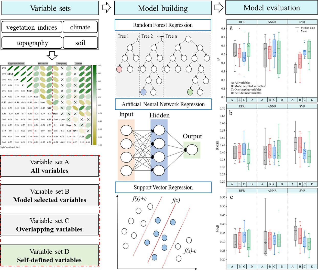
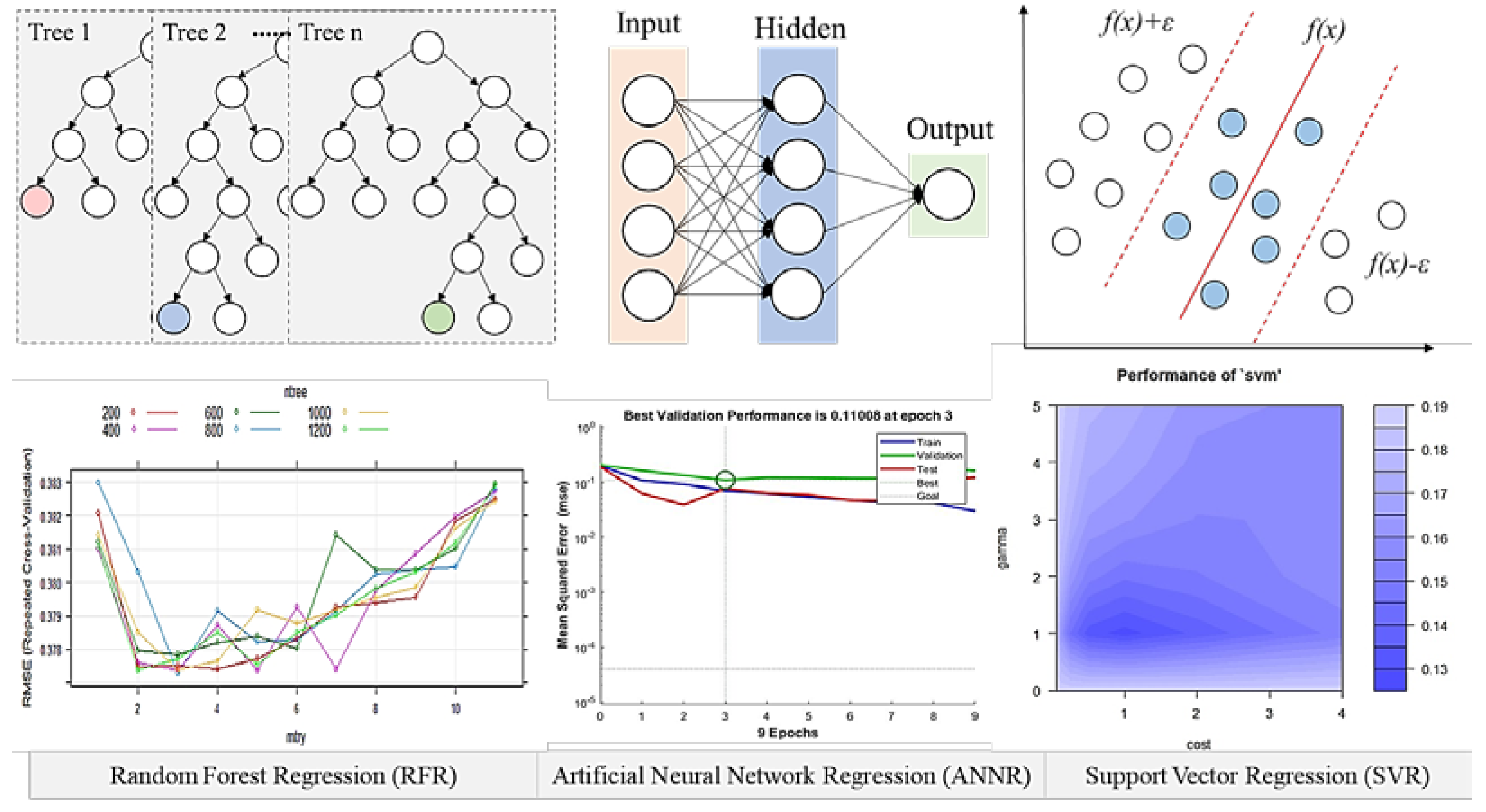
2.3. Machine Learning Algorithms and Measure of Variable Importance Methods

2.3.1. Random Forest Regression

The Random Forest (RF) is an integrated algorithm for unpruned classification or regression trees created using bootstrap samples of training data and random feature selection in tree induction proposed by Breiman [38,39]. It contains a metric for ranking importance values, and the importance of each variable can be calculated in two different ways, including increase in node purity (IncNodePurity) and increase in mean squared error (%IncMSE) [40]. In both algorithms, higher values indicate that the variable is more important. The IncNodePurity is measured by the sum of squared residuals, representing the effect of each variable on the heterogeneity of observations at each node of the classification tree, and thus comparing the importance of the variable. The %IncMSE is measured by the error increased to the model prediction through randomly assigning a value to each predictor variable that is more important if it is replaced at random. There are some differences in the ranking of the importance of the variables derived from the two methods. In this study, the %IncMSE method was used to estimate the relative importance of a particular variable [29]. In particular, two important hyperparametric tree predictors (ntree) and split nodes (mtry) need to be optimized in the RFR model [41] to obtain tuning parameters and accuracy evaluations using the grid search and CV processes. The analysis was performed using the “Random Forest” package in the statistical package R 4.1.1.

2.3.2. Artificial Neural Network Regression

The Artificial Neural Networks (ANNs) are non-linear statistical learning methods and are one of the most commonly used modelling techniques with a highly interconnected structure, similar to the human brain, that mimics the operation and connectivity of biological neurons [42]. This refers to a multilayer network structure consisting of an input layer, an output layer and a hidden layer. The mean impact value (MIV) method is one of the best indicators for evaluating the correlation of variables in ANNs. The MIV reflects the changes in the weight matrix of each variable in the neural network and allows a quantitative evaluation of the importance of each independent variable on the influence of the dependent variable [43]. The absolute magnitude represents the relative weight of the influence of the respective variable on the dependent variable. In ANNR, to design the network for optimal topology, the optimal numbers of hidden layers and neurons are determined based on a trial-and-error process [44]. The analysis was performed using the “nnet” package in the statistical package R 4.1.1.

2.3.3. Support Vector Regression

The support vector machine is a relatively simple supervised MLAs to solve classification or regression problems proposed by Cortes and Vapnik in 1995 [45]. The essence of the support vector regression (SVR) is to find a hyperplane between different data types to create boundaries. In two-dimensional space, this hyperplane is a straight line. Compared to traditional methods, SVR can handle high-dimensional data better with relatively few training samples and can generalize complex models. In SVR, the two parameters, gamma and cost, affect the model’s performance [46]. We selected the parameters with the lowest errors as the optimal parameter combination by the grid search method to obtain the error deviations under different parameter combinations. The analysis was performed using the “e1071” package in the statistical package R 4.1.1. Use the “rminer” package to generate a regression model of the importance of the variables.

2.4. Performance Evaluation of the Model

We used the coefficient of determination (R2), root mean square error (RMSE), and mean absolute error (MAE) as measures based on the 10-fold cross validation method to evaluate the performance of each model. The sample plots were split into 10 datasets of equal numbers of plots, and these measures were calculated for each dataset. This process was repeated 10 times to ensure that all the data were involved in the training of the model and the validation of the results. Finally, these measurements were averaged to obtain the final R2, RMSE and MAE values of each model. Higher R2 and lower RMSE values indicate that the model has a better precision in LAI estimation. R2, RMSE and MAE values can be expressed as follows:
R 2 = 1 i = 1 n ( y i y i ) 2 i = 1 n ( y i y ¯ i ) 2
R M S E = 1 n i = 1 n ( y i y i ) 2
MAE = 1 n i = 1 n | y i y i |
where y i is the predicted LAI, y i is the measured LAI, y i ¯ is the measured mean values of LAI and n is the number of measured LAI in the validation dataset.

3. Results

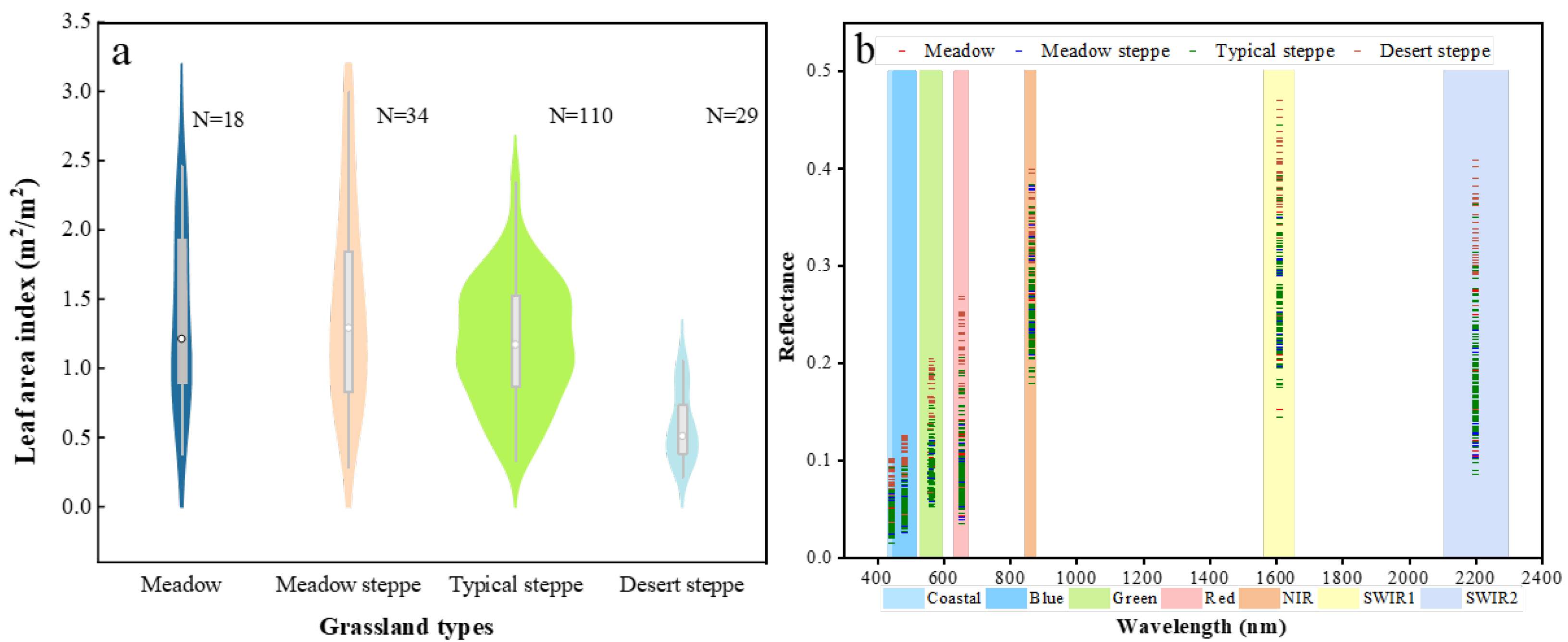
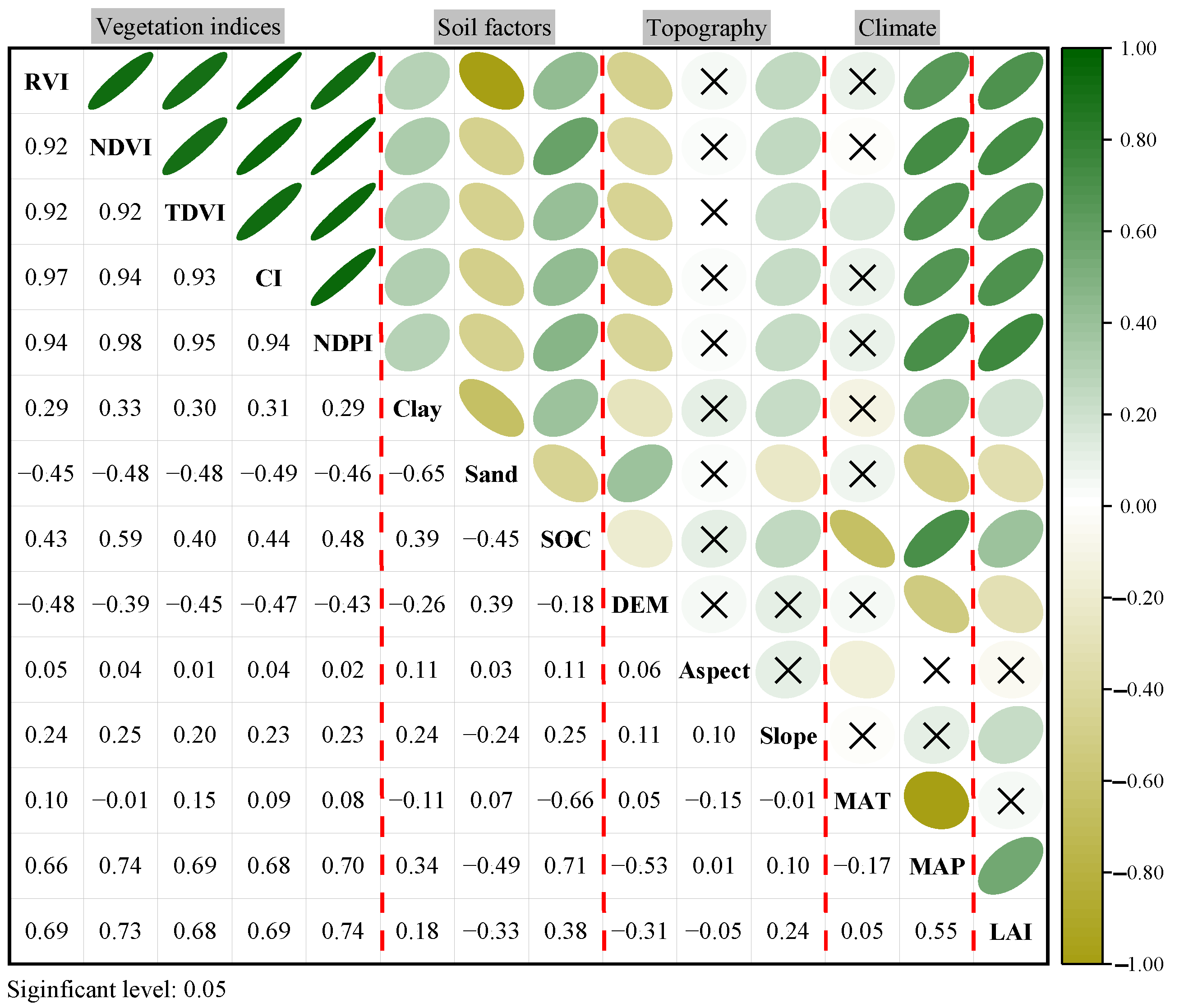
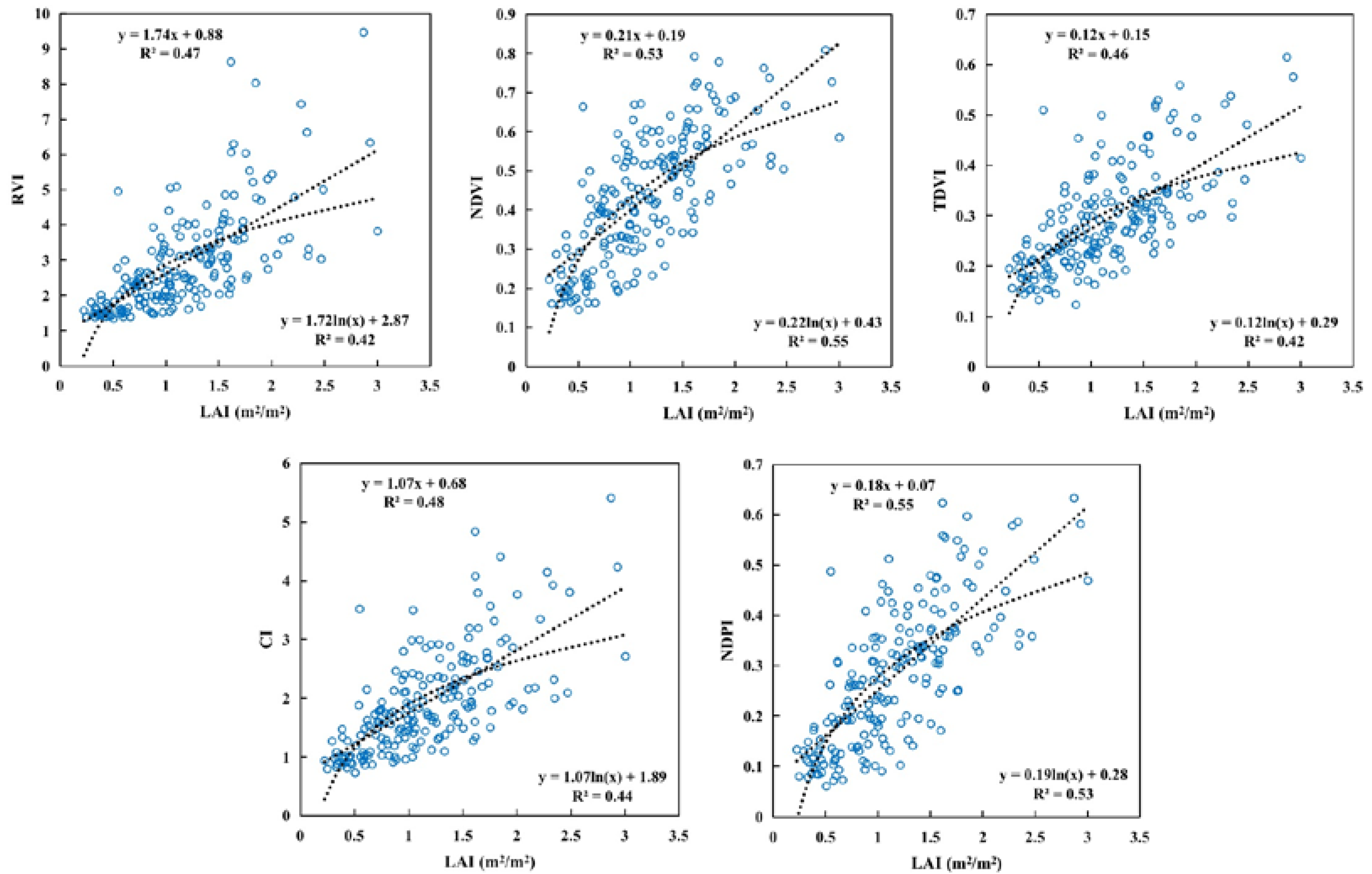
3.1. In Situ LAI Characteristics and Correlation Analysis

Of all the sample plots, 18 sample plots were distributed in meadow, 34 in meadow steppe, 110 in typical steppe and 29 in desert steppe (Figure 2a). According to the Shapiro–Wilk normality test, the four datasets all conformed to a normal distribution. Generally, the mean values of the in situ LAI ranged from 0.22 to 3.01 m2/m2 among all sample plots. The LAI values in meadow ranged from 0.38 to 2.47 m2/m2 with a mean value of 1.35 m2/m2; in meadow steppe, the mean and variability of LAI values were relatively high, with a mean LAI value of 1.45 m2/m2; in typical steppe, the LAI values had a distribution range of 0.34–2.34 m2/m2 with a mean value of 1.18 m2/m2. The LAI values of desert steppe had a minimum value of 0.22 m2/m2 and a maximum value of 1.06 m2/m2 with a mean value of 0.57 m2/m2. The reflectance of the sample plots had the widest range of variation in the SWIR1 and SWIR2 bands. The SWIR1 band reflectance was generally used to calculate the VIs (Figure 2b).
Pearson correlation coefficients were used to explore the relationship between LAI and multiple variables. We initially selected a total of 13 variables, covering VIs, soil factors, climate factors and topography factors. The VIs included RVI, NDVI, TDVI, CI and NDPI. Soil factors included soil organic carbon content (SOC), clay content (Clay) and sand gravel content (Sand) of topsoil (0–20 cm). Topography factors included elevation (DEM), slope (Slope) and aspect (Aspect). Climate factors included annual mean temperature (MAT) and precipitation (MAP) from 2000 to 2019. Of the 13 variables, only Aspect and MAT were not correlated with LAI at the 0.05 level of significance. After the above analysis, 11 predictive variables were chosen to train the models, which were significantly correlated with the measured LAI. These VIs were all significantly positively correlated with LAI, with NDPI having the highest correlation with LAI (r = 0.74). DEM was significantly negatively correlated with LAI (r = −0.31). MAP was significantly positively correlated with LAI (r = 0.55), and Clay and SOC were both significantly positively correlated with LAI with correlation coefficients of 0.18 and 0.38, respectively. Sand was significantly negatively correlated with LAI (r = −0.33), as shown in Figure 3.

3.2. Variable Importance

Prior to using the MLAs, optimal tuning of the model parameters was carried out to improve the stability, reliability and generalization of the model results. The optimum parameters for both the RFR, ANNR and SVR approaches were chosen. See Section 2.3 for details of the method for selecting the parameters for each MLAs. In this study, for RFR, we found that the model performed better when ntree was set to 3 and the mtry was set to 800. For ANNR, after several trials, we found that using the hidden layer model containing 1 neuron performed the best. For SVR, we found that it performed best when the cost was set to 1 and the gamma was set to 0.1 (Figure 4). Other parameters used the default values from the packages.
Table 2 illustrates the relative importance of the input variables to the LAI estimates in the RFR, ANNR and SVR models. All variables involved in training were ranked. A common feature of the results from all the importance ranking methods was that these VIs were in the top of the ranking. NDPI which takes SWIR into consideration was the best performer of all models, followed by NDVI, with the other variables performing inconsistently. For the RFR and SVR models, MAP was also a relatively important variable. However, the importance ranking of MAP in the ANNR model was relatively low. DEM was not high in the importance ranking of all three models.

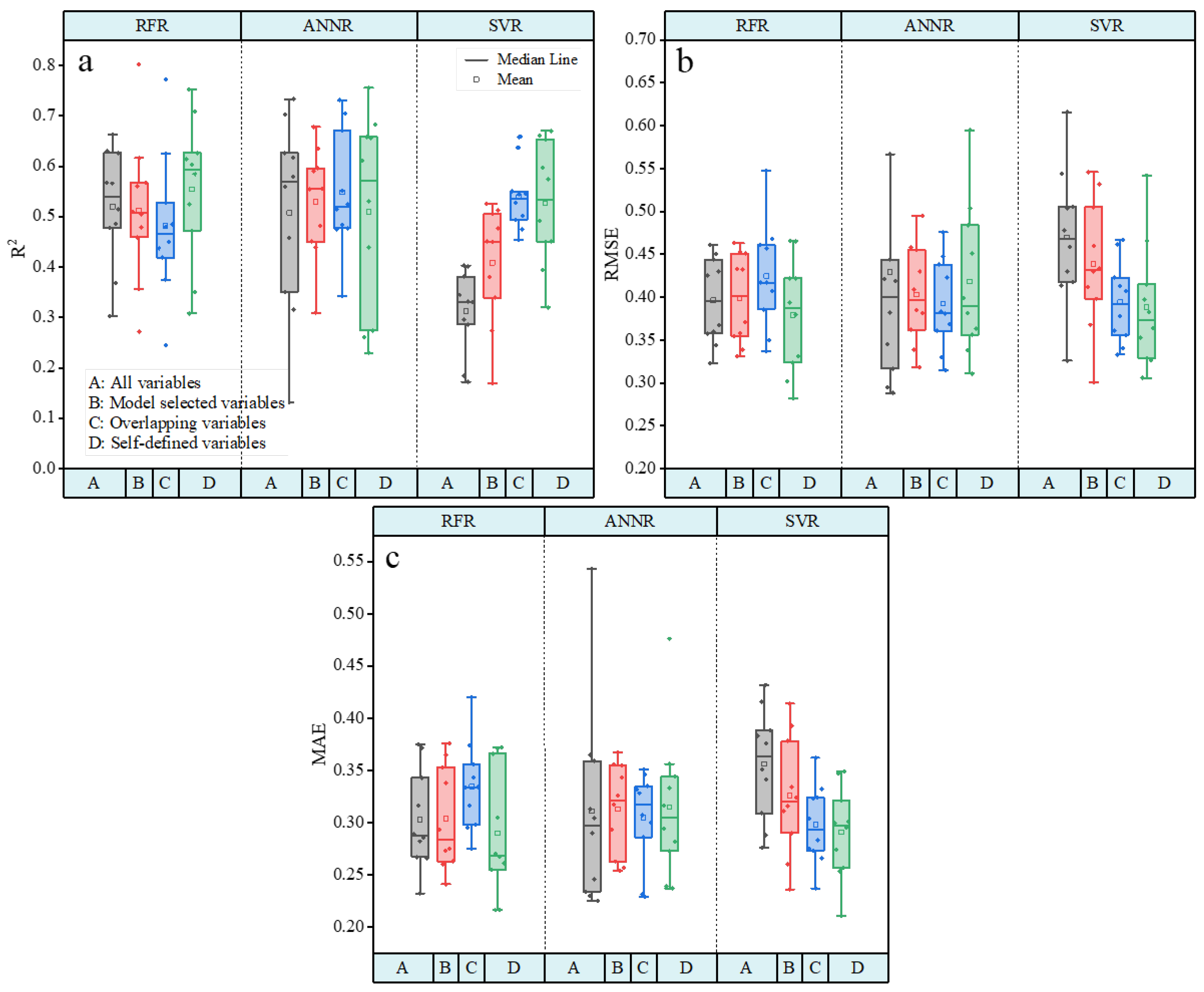
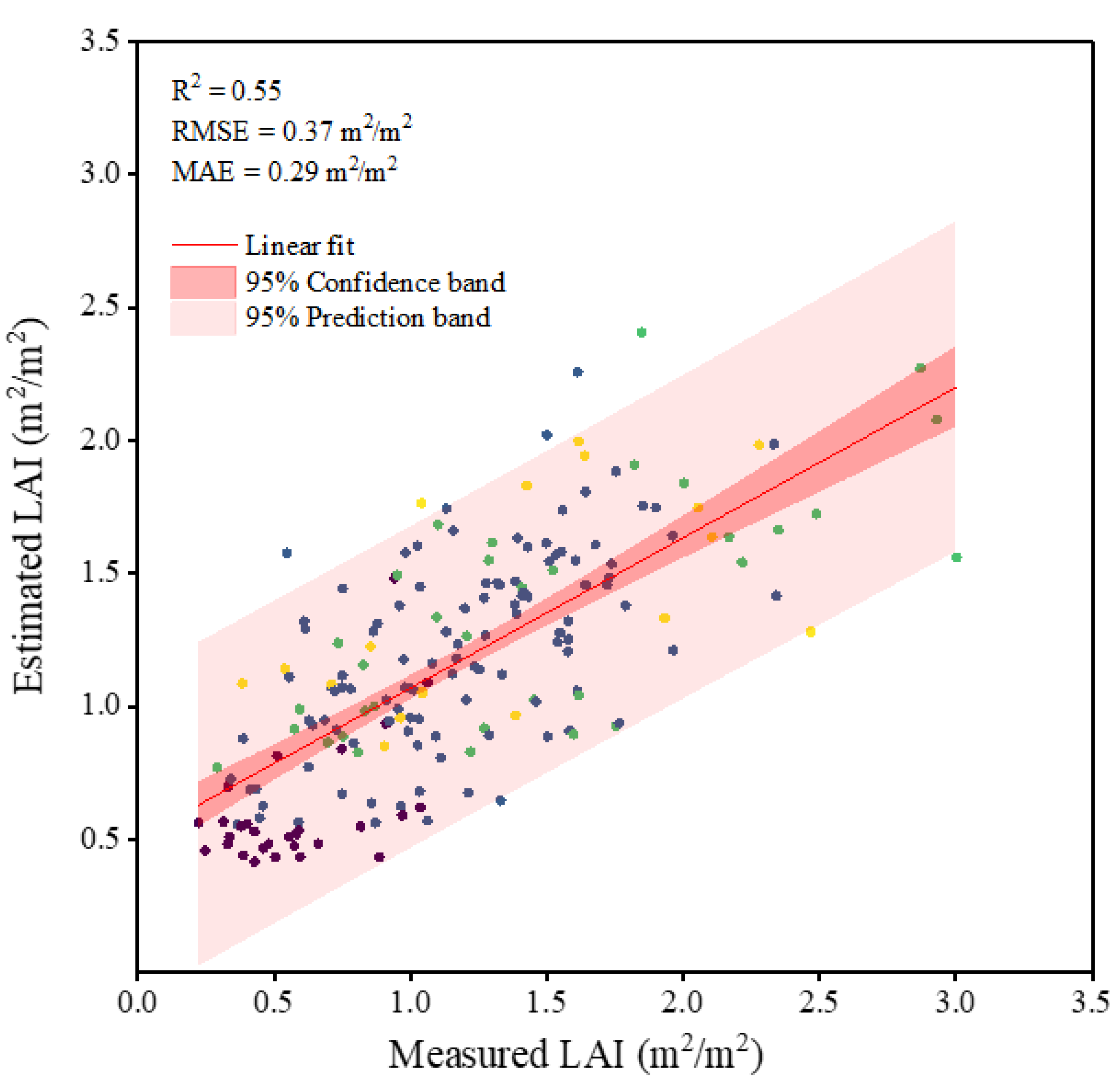
3.3. Model Building and Evaluation

We established four variable sets to compare and select the best independent variable combination. Variable set A covered all variables listed in Table 2. Variable set B included the top five variables ranked by importance in RFR, ANNR and SVR, respectively, with a cumulative mean impact value of at least 85% based on ANNR. Variable set C is the overlapping variables in variable set B of the three methods, which included NDPI and NDVI in this study. These mentioned variable sets were established on statistical or mathematical methods. Some variables with an empirically significant relationship with vegetation growth such as SOC, DEM and MAP were excluded. Meanwhile, the NDPI and the NDVI had a significant relationship (r = 0.98). Therefore, variable set D was a self-defined combination of variables incorporating empirical knowledge, which included NDPI, MAP, SOC and DEM and they were both mathematically and empirically selected variables. Thus, we compared 12 models in total including three machine learning models (RFR, ANNR and SVR) with different numbers of input variables (A: all variables, B: model selected variables, C: overlapping variables and D: self-defined variables). The evaluation results of 12 models (RFR-A, RFR-B, RFR-C, etc.) derived from 10-fold cross validation method with respect to R2, RMSE and MAE are displayed in Figure 5.
Among these 12 models, simulated LAI showed a significant correlation with observed LAI, with R2 ranging from 0.31 to 0.55, RMSE ranging from 0.37 to 0.47 m2/m2 and MAE ranging from 0.29 to 0.36 m2/m2. Among the three MLAs, the RFR model showed a higher prediction accuracy, followed by ANNR, and SVR was less effective in simulating the LAI in this study. Overall, the RFR model when NDPI, SOC, DEM and MAP were used as input variables performed the best, with the highest R2 (0.55) and lowest RMSE (0.37 m2/m2) and MAE (0.29 m2/m2). Subsequently, the results of the model’s 10-fold cross validation test sets were pooled together to produce scatter plots of different grassland types, as shown in Figure 6. The results show that the confidence interval was narrowest in areas with LAI close to the mean value (1.17 m2/m2). Prediction uncertainty increased as the LAI of grassland deviated from the mean value.

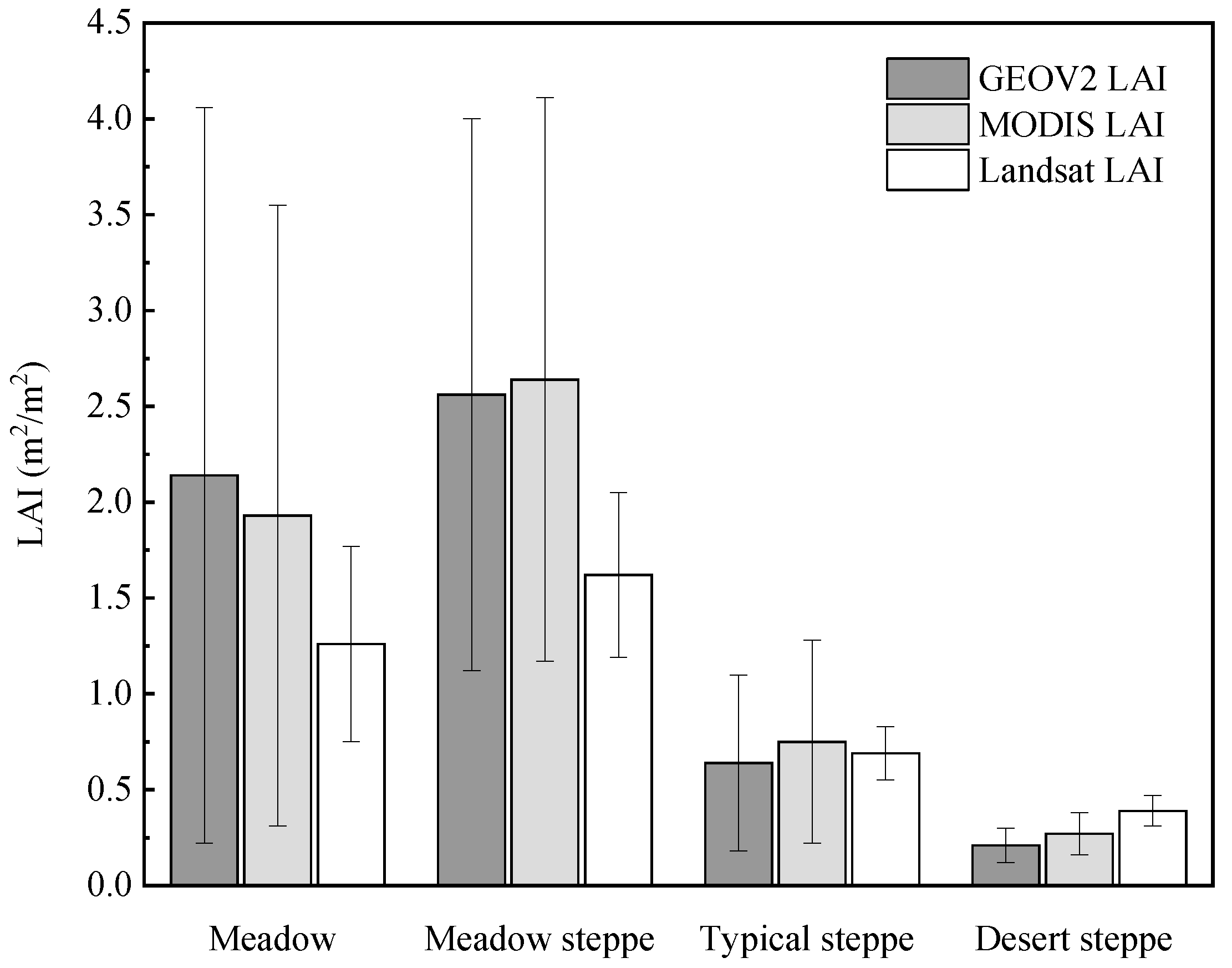
3.4. Intercomparison with Other LAI Products

We used the highest accuracy model (RFR-D) develop the spatial distribution of LAI map (named the Landsat LAI). To better ensure the consistency across time of the three products, we selected four sub-regions based on the spatial distribution of different grassland types in Inner Mongolia to analyze the result of the model inversions chosen in this study for comparison with MODIS LAI and GEOV2 LAI (Table 3, Figure 7a). The dates of the two selected products storage were not recorded in the same way: MODIS LAI was recorded at an 8-day temporal resolution and GEOV2 LAI was recorded at a 10-day temporal resolution. This study for comparison recorded the time in year-month-day and it should be noted that the time two products corresponded to the date for the time resolution which corresponded to the last day of the date (Table 3). In order to directly compare Landsat LAI, MODIS LAI and GEOV2 LAI products, they were resampled to the same spatial resolution of 1 km. The distribution area of the magnitude of LAI values was consistent, showing a trend of high northeast and low southwest in the four scenes, but Landsat LAI with the resolution of 30 m showed more detail and MODIS LAI had more invalid pixels (Figure 7b). The spatial distribution of LAI in terms of the grassland types also correlated closely with our observations in the field survey.
Figure 8 shows the intercomparison of grassland LAI in the four sub-regions among MODIS LAI, GEOV2 LAI products and up-scaled Landsat LAI. Related studies have shown that the GEOV2 LAI product performed better on grassland, and the results derived from this study were used to compare with this product. There was a similar spatial distribution for both products. A larger spatial variation was found in MODIS LAI compared to the other products. Among the different grassland types, all three LAI products showed a consistent trend, with meadow steppe being the highest, followed by meadow, followed by typical steppe, with desert steppe row being the smallest. In addition, the LAI in this study produced larger LAI values in the desert steppe and smaller LAI values in the other grassland types. The Landsat LAI had the smallest standard deviation among the three products. The modelling in this study was for the overall modelling of the sample plots and was not split into different grassland types. According to the results of this study, we found that there was a difference among different grassland types. The next study will be modelled for different grassland types.

4. Discussion

In this study, the initially selected variables covered VIs, climate factors, soil factors and topography factors. The VIs included the RVI, the NDVI, the TDVI, the CI and the NDPI, which both had strong relationships with the in situ measured LAI (Figure 3). Meanwhile, these VIs have been proven to be advantageous in estimating vegetation biophysical characteristics calculated from remotely sensed data [26,29]. The NDVI was regarded as the most popular vegetation index among these Vis; however, it is strongly influenced by soil reflectance at low LAI and its sensitivity decreases rapidly with increasing LAI due to the light absorption in the red band became saturated at high LAI [33,47]. The CI is a vegetation index created to estimate the chlorophyll content, which is calculated by the reflectance in green and near-infrared band [33]. The NDPI is a new vegetation index that was proposed in 2017 which has good advantages in the inversion of biomass and the fraction of absorbed photosynthetically active radiation and is also proving to have great potential for application [34,48,49]. Linear and logarithmic relationships between the in situ measured LAI including all sample plots and these VIs are shown in Figure 9. It can be seen that the saturation issue between the LAI and VIs was not evident in this study; the linear regression models presented greater R2 values than logarithmic regression models except for the NDVI, perhaps because the LAI values used for modeling were between 0.22 and 3.01 m2/m2, which do not easily reach saturation, and related studies have shown that a tendency to saturation begins to occur at higher LAI. The NDVI and NDPI had a comparable R2 for linear and nonlinear regression models. NDPI can be used in LAI estimation with the aim of increasing the sensitivity of high LAI areas and reducing the effect the soil background [34]. The NDPI significantly reduced the soil impact on VIs across large and heterogeneous grassland areas. It also indicates that NDPI performed better in the inversion of LAI than the other VIs in this study. Furthermore, NDPI was ranked first and entered the model as a variable regardless of the importance ranking method used (Table 2). Thus, we consider NDPI to be a promising vegetation index for LAI estimation.
MLAs have been widely used in recent years. The RFR model showed a higher prediction accuracy, followed by ANNR and SVR, in simulating the LAI of Inner Mongolia grassland in this study (Figure 5). The good performance of RFR has been demonstrated in several published studies [26,50,51]. The RFR is insensitive to noise and overfitting, and can model complex relationships with fewer parameters, resulting in a superior performance compared to other regression algorithms. The selection of input variables had a great impact on the estimation performance of MLAs. Analysis of the vegetation growth process showed that the influence factors ranged from climate to soil until the topography factors. In the satellite-based LAI inversion process, both the color and texture of the soil affected the inversion results, so the SOC, Clay and Sand were chosen as representative indicators. The response of vegetation to climate change is very sensitive, and LAI, as an important parameter of vegetation ecosystem, can also indirectly reflect climate change and this phenomenon is particularly obvious in arid regions [7]. MAP and MAT illustrate the climate condition. The grassland in Inner Mongolia is all relatively flat and less affected by elevation. The importance of DEM was not ranked high in any of the three algorithms. In addition, these VIs were a reflection of the vegetation growth condition. We obtained a total of 13 variables, but it was not necessary to apply them all to the model building. When it comes to the select of the variables in the models, it should not only depend on the result of the machine learning. The principle of selecting variables should be to comprehensively consider the growth environment of grassland and to adequately select representative indicators that influence their growth factors. Nevertheless, the machine learning approach selected parameters ignoring the vegetation growth process and was based on the statistical results of the input data. When the variables with large importance values were selected by MLAs, VIs tended to be ranked first; meanwhile, among the four types of factors, VIs had the highest correlation coefficient with the in situ measured LAI (Table 2, Figure 3), and there was a significant correlation between different VIs after different combinations of bands when the calculation was performed with a relatively single factor. This is because VIs reflect reflectance and LAI is a determinant factor of canopy reflectance [52]. If the selection of variables involved in the modeling relied only on the importance ranking results, this would affect the simulation results of the model as the variables might be limited to one class of factors (Table 2). Therefore, the factors selected by adding empirical knowledge are involved in training the models and comparing them with other results to assess the differences between the models. Published studies have shown the underlying mechanisms of using these variables to estimate grassland LAI from remotely sensed data and that their contribution to grassland LAI estimates is the result of the combined effect of soil, climate and topography [53]. To quantify the contribution of the improvement of the estimation, we built the 12 different LAI estimation models. The results also demonstrated that the model was simulated by considering multiple factors such as NDPI, SOC, DEM and MAP which were used as regression variables and their correlation was not the best, with LAI offering better results (Figure 5). Using MLAs to scale field-measured LAI through high-resolution imagery to larger pixel sizes for comparison with medium-resolution products can bridge the scale difference between ground-based LAI measurements and medium-resolution pixels and can therefore be used as a method of scale conversion [4]. There was covariance between the indices selected according to the machine learning approach. The set of indicators constructed according to a priori knowledge was used to build the model expressions with more comprehensive information. The data covered a wide range of factors and were the result of a combination of multiple factors driving the model expressions. In summary, the model expressions with the combination of several strengths were also optimal. According to the statistical results, among the 12 LAI estimation models, the RFR-D had the highest accuracy. Meanwhile, this result was also consistent with the above analysis and in line with our expectations.
We chose two widely used LAI products to compare our results with. In the process of comparison between MODIS LAI and GEOV2 LAI, we found that they had a good agreement, which was strongly related to the algorithms used in their production produce process. GEOV2 LAI in the production process of MODIS LAI data when it is used as training data will cause the two datasets to have a strong consistency [35,36]. At the same time, the two products are global data, so not representative of the grassland. Our results were based on in situ measured LAI, the spatial resolution was high and the regional LAI distribution was persuasive. All the LAI products showed a consistent trend, with the LAI in the meadow steppe being the highest, followed by the meadow, followed by the typical steppe, and the LAI in the desert steppe was the smallest (Figure 8). This was mainly caused by the obvious spatial heterogeneity in the distribution of vegetation resources, which reflected the spatial complexity and variability of ecosystem properties which form spatial patterns that are closely related to ecosystem functions and processes [10]. The validation of LAI products is critical to the use of satellite-based LAI products. Fang et al., [54] found that the uncertainties of current LAI products still do not meet the accuracy demand of GCOS. Validation of LAI products continues to be an important element. With respect to the limitations in this study, data from only one time node were selected for comparison with other products, and subsequent inversions of long time series should be performed for a more comprehensive comparison and analysis. Comparative validations for more products in the grassland applications will be carried out in the next step. The LAI of different grassland types has significant differences. Due to the limited number of field sample plots in this paper, a unified model was adopted to simulate LAI. In the future, more data should be collected to establish models separately for different grassland types. Since the image quality can be affected by cloudy weather, multi-source data fusion should be considered in the process of acquiring long time series data [55].

5. Conclusions

This study explored the results of different importance value ranking methods for all variables, and compared the simulation results of different datasets as input data for RFR, ANNR and SVR. Finally, two widely used LAI products were selected for a comparative analysis. Based on three different algorithms for ranking the importance of all variables, the sort of all variables was different. Among all the variables, NDPI was always ranked in the first place, which was calculated by the reflectance of NIR and SWIR bands. It had good advantages in the inversion of vegetation characteristics and was also proven to have great potential for application. In the simulation of the LAI in Inner Mongolia grassland, the RFR showed a higher prediction accuracy, followed by ANNR and SVR. The highest model accuracy (R2 = 0.55, RMSE = 0.37 m2/m2, MAE = 0.29 m2/m2) was based on a combination dataset of the self-defined variables and RFR. Using MLAs, multi-factor models have advantages over single-factor models in simulating vegetation characteristics. The self-defined variables contain more information than the set of variables selected by the machine learning approach. Intercomparison with MODIS LAI and GEOV2 LAI products showed that the LAI in this study produced larger values in the desert steppe and smaller values in the others. However, it had the smaller standard deviation and the differences between the three products were consistent across the four sub-regions. In general, our results demonstrated that MLAs incorporating empirical knowledge could improve the accuracy of modelling LAI and provide guidance for LAI modeling and the validation of LAI products. However, the application of this approach to regional mapping needs to be further explored.

Author Contributions

Conceptualization, B.S., X.X. and X.W.; methodology, B.S. and L.D.; software, B.S.; validation, B.S. and Z.L.; formal analysis, B.S. and L.D.; resources, X.X., D.X. and L.M.; data curation, B.S. and Z.L.; writing—original draft preparation, B.S. and L.H.; writing—review and editing, B.S., A.P., Z.K., J.C. and S.M.; supervision, X.X. All authors have read and agreed to the published version of the manuscript.

Funding

This study was supported by the National Key Research and Development Program of China (2021YFD1300500, 2021YFF0703904); the National Natural Science Foundation of China (32130070, 31971769, 41771205, 42101372); the Special Funding for Modern Agricultural Technology Systems from the Chinese Ministry of Agriculture (CARS-34); the Fundamental Research Funds Central Non-profit Scientific Institution (1610132021016).

Institutional Review Board Statement

Not applicable.

Informed Consent Statement

Not applicable.

Data Availability Statement

The data presented in this study are available on request from the corresponding author.

Acknowledgments

We are grateful to many colleagues with the Hulunber Grassland Ecosystem Observation and Research Station, Institute of Agricultural Resources and Regional Planning, Chinese Academy of Agricultural Sciences (CAAS). We acknowledge the assistance of Shen Jie, students of CAAS and Li Zhipeng, Tao Jifeng, students at Baotou Teachers’ College, in the field observation and sample collection. Acknowledgment is given for the data support from “National Earth System Science Data Center, National Science and Technology Infra-structure of China. (http://www.geodata.cn, accessed on 29 January 2022)”.

Conflicts of Interest

The authors declare no conflict of interest.

References

  1. Scurlock, J.M.O.; Hall, D.O. The global carbon sink: A grassland perspective. Glob. Chang. Biol. 2010, 4, 229–233. [Google Scholar] [CrossRef]
  2. Watson, D.J. Comparative and physiological studies on growth of field crop variation in net assimilation rate and leaf area between species and varieties and within years. Ann. Bot. 1947, 11, 41–76. [Google Scholar] [CrossRef]
  3. Chen, J.M.; Black, T.A. Defining leaf area index for non-flat leaves. Plant Cell Environ. 1992, 15, 421–429. [Google Scholar] [CrossRef]
  4. Fang, H.L.; Baret, F.; Plummer, S.; Schaepman-Strub, G. An overview of global leaf area index (LAI): Methods, products, validation, and applications. Rev. Geophys. 2019, 57, 739–799. [Google Scholar] [CrossRef]
  5. Wang, Y.J.; Woodcock, C.E.; Buermann, W.; Stenberg, P.; Voipio, P.; Smolander, H.; Häme, T.; Tian, Y.H.; Hu, J.N.; Knyazikhin, Y.; et al. Evaluation of the MODIS LAI algorithm at a coniferous forest site in Finland. Remote Sens. Environ. 2004, 91, 114–127. [Google Scholar] [CrossRef]
  6. Sellers, P.J.; Dickinson, R.E.; Randall, D.A.; Betts, A.K.; Hall, F.G.; Berry, J.A.; Collatz, G.J.; Denning, A.S.; Mooney, H.A.; Nobre, C.A.; et al. Modeling the exchanges of energy, water, and carbon between continents and the atmosphere. Science 1997, 275, 502–509. [Google Scholar] [CrossRef] [PubMed]
  7. Chase, T.N.; Pielke, R.A.; Kittel, T.G.F.; Nemani, R.; Running, S.W. Sensitivity of a general circulation model to global changes in leaf area index. J. Geophys. Res.: Atmos. 1996, 101, 7393–7408. [Google Scholar] [CrossRef]
  8. Thornton, P.K.; Ericksen, P.J.; Herrero, M.; Challinor, A.J. Climate variability and vulnerability to climate change: A review. Glob. Chang. Biol. 2014, 20, 3313–3328. [Google Scholar] [CrossRef] [PubMed]
  9. Liang, T.G.; Yang, S.X.; Feng, Q.S.; Liu, B.K.; Zhang, R.P.; Huang, X.D.; Xie, H.J. Multi-factor modeling of above-ground biomass in alpine grassland: A case study in the Three-River Headwaters Region, China. Remote Sens. Environ. 2016, 186, 164–172. [Google Scholar] [CrossRef]
  10. Chen, Y.F.; Dong, M. Spatial heterogeneity in ecological systems. Ecol. Sin. 2003, 23, 346–352. [Google Scholar] [CrossRef]
  11. Martínez, B.; García-Haro, F.J.; Coca, F.C. Derivation of high-resolution leaf area index maps in support of validation activities: Application to the cropland Barrax site. Agric. For. Meteorol. 2009, 149, 130–145. [Google Scholar] [CrossRef]
  12. Weiss, M.; Baret, F.; Smith, G.J.; Jonckheere, I.; Coppin, P. Review of methods for in situ leaf area index (LAI) determination: Part II. Estimation of LAI, errors and sampling. Agric. For. Meteorol. 2004, 121, 37–53. [Google Scholar] [CrossRef]
  13. Jonckheere, I.; Fleck, S.; Nackaerts, K.; Muys, B.; Coppin, P.; Weiss, M.; Baret, F. Review of methods for in situ leaf area index determination: Part I. Theories, sensors and hemispherical photography. Agric. For. Meteorol. 2004, 121, 19–35. [Google Scholar] [CrossRef]
  14. Zhang, B. Current status and future prospects of remote sensing. Bull. Chin. Acad. Sci. 2017, 32, 774–784. [Google Scholar]
  15. Li, X.C.; Xu, X.G.; Bao, Y.S.; Huang, W.J.; Luo, J.H.; Dong, Y.Y.; Song, X.Y.; Wang, J.H. Retrieving LAI of winter wheat based on sensitive vegetation index by the segmentation method. Sci. Agric. Sin. 2012, 45, 3486–3496. [Google Scholar]
  16. Li, K.L.; Jiang, J.J.; Mao, R.Z.; Ni, S.X. The modeling of vegetation through leaf area index by means of remote sensing. Acta Ecol. Sin. 2005, 25, 1491–1496. [Google Scholar]
  17. Fang, H.L.; Liang, S.L.; Kuusk, A. Retrieving leaf area index using a genetic algorithm with a canopy radiative transfer model. Remote Sens. Environ. 2003, 85, 257–270. [Google Scholar] [CrossRef]
  18. Verrelst, J.; Malenovský, Z.; Tol, C.V.; Camps-Valls, G.; Gastellu-Etchegorry, J.P.; Lewis, P.; North, P.; Moreno, J. Quantifying vegetation biophysical variables from imaging spectroscopy data: A review on retrieval methods. Surv. Geophys. 2019, 40, 589–629. [Google Scholar] [CrossRef]
  19. Verrelst, J.; Camps-Valls, G.; Muñoz-Marí, J.; Rivera, J.P.; Veroustraete, F.; Clevers, J.G.P.W.; Moreno, J. Optical remote sensing and the retrieval of terrestrial vegetation bio-geophysical properties—A review. ISPRS J. Photogramm. 2015, 108, 273–290. [Google Scholar] [CrossRef]
  20. Baret, F.; Buis, S. Estimating Canopy Characteristics from Remote Sensing Observations: Review of Methods and Associated Problems; Springer: Dordrecht, The Netherlands, 2008. [Google Scholar] [CrossRef]
  21. Durbha, S.S.; King, R.L.; Younan, N.H. Support vector machines regression for retrieval of leaf area index from multiangle imaging spectroradiometer. Remote Sens. Environ. 2007, 107, 348–361. [Google Scholar] [CrossRef]
  22. Verrelst, J.; Muñoz, J.; Alonso, L.; Delegido, J.; Rivera, J.P.; Camps-Valls, G.; Moreno, J. Machine learning regression algorithms for biophysical parameter retrieval: Opportunities for Sentinel-2 and -3. Remote Sens. Environ. 2012, 118, 127–139. [Google Scholar] [CrossRef]
  23. Jalonen, J.; Järvelä, J.; Virtanen, J.P.; Vaaja, M.; Kurkela, M.; Hyyppä, H. Determining characteristic vegetation areas by terrestrial laser scanning for floodplain flow modeling. Water 2015, 7, 420–437. [Google Scholar] [CrossRef] [Green Version]
  24. Berterretche, M.; Hudak, A.T.; Cohen, W.B.; Maiersperger, T.K.; Gower, S.T.; Dungan, J. Comparison of regression and geostatistical methods for mapping Leaf Area Index (LAI) with Landsat ETM+ data over a boreal forest. Remote Sens. Environ. 2005, 96, 49–61. [Google Scholar] [CrossRef]
  25. Zhong, S.F.; Zhang, K.; Bagheri, M.; Burken, J.G.; Gu, A.; Li, B.K.; Ma, X.M.; Marrone, B.L.; Ren, Z.Y.J.; Schrier, J.; et al. Machine Learning: New ideas and tools in environmental science and engineering. Environ. Sci. Technol. 2021, 55, 12741–12754. [Google Scholar] [CrossRef]
  26. Li, Z.W.; Wang, J.H.; Tang, H.; Huang, C.Q.; Yang, F.; Chen, B.R.; Wang, X.; Xin, X.P.; Ge, Y. Predicting grassland leaf area index in the meadow steppes of northern China: A comparative study of regression approaches and hybrid geostatistical methods. Remote Sens. 2016, 8, 632. [Google Scholar] [CrossRef]
  27. Han, Z.Y.; Zhu, X.C.; Fang, X.Y.; Wang, Z.Y.; Wang, L.; Zhao, G.X.; Jiang, Y.M. Hyperspectral estimation of apple tree canopy LAI based on SVM and RF regression. Spectrosc. Spectr. Anal. 2016, 36, 800–805. [Google Scholar]
  28. Pullanagari, R.R.; Kereszturi, G.; Yule, I.J. Mapping of macro and micro nutrients of mixed pastures using airborne AisaFENIX hyperspectral imagery. ISPRS J. Photogramm. 2016, 117, 1–10. [Google Scholar] [CrossRef]
  29. Ding, L.; Li, Z.W.; Shen, B.B.; Wang, X.; Xu, D.W.; Yan, R.R.; Yan, Y.C.; Xin, X.P.; Xiao, J.F.; Li, M.; et al. Spatial patterns and driving factors of aboveground and belowground biomass over the eastern Eurasian steppe. Sci. Total Environ. 2022, 803, 149700. [Google Scholar] [CrossRef]
  30. Jordan, C.F. Derivation of leaf-area index from quality of light on the forest floor. Ecology 1969, 50, 663–666. [Google Scholar] [CrossRef]
  31. Rouse, J.W., Jr.; Haas, R.H.; Schell, J.A.; Deering, D.W. Monitoring Vegetation System in the Great Plains with ERTS; Goddard Space Flight Center 3d ERTS-1 Symposium; NASA: Washington DC, USA, 1974; Volume 1, pp. 309–317. [Google Scholar]
  32. Bannari, A.; Asalhi, H.; Teillet, P.M. Transformed difference vegetation index (TDVI) for vegetation cover mapping. In Proceedings of the IEEE International Geoscience & Remote Sensing Symposium, Toronto, ON, Canada, 24–28 June 2002; pp. 3053–3055. [Google Scholar]
  33. Gitelson, A.A.; Vina, A.; Arkebauer, T.J.; Rundquist, D.C.; Keydan, G.; Leavitt, B. Remote estimation of leaf area index and green leaf biomass in maize canopies. Geophys. Res. Lett. 2003, 30, 1248. [Google Scholar] [CrossRef]
  34. Wang, C.; Chen, J.; Wu, J.; Tang, Y.H.; Shi, P.J.; Black, T.A.; Zhu, K. A snow-free vegetation index for improved monitoring of vegetation spring green-up date in deciduous ecosystems. Remote Sens. Environ. 2017, 196, 1–12. [Google Scholar] [CrossRef]
  35. Myneni, R.B.; Hoffman, S.; Knyazikhin, Y.; Privette, J.L.; Glassy, J.; Tian, Y.; Wang, Y.; Song, X.; Zhang, Y.; Smith, G.R.; et al. Global products of vegetation leaf area and fraction absorbed PAR from year one of MODIS data. Remote Sens. Environ. 2002, 83, 214–231. [Google Scholar] [CrossRef]
  36. Baret, F.; Weiss, M.; Lacaze, R.; Camacho, F.; Makhmara, H.; Pacholcyzk, P.; Smets, B. GEOV1: LAI and FAPAR essential climate variables and FCOVER global time series capitalizing over existing products. Part1: Principles of development and production. Remote Sens. Environ. 2013, 137, 299–309. [Google Scholar] [CrossRef]
  37. DAHV (Department of Animal Husbandry and Veterinary, the Ministry of Agriculture of the People’s Republic of China); NAHVS (National Animal Husbandry and Veterinary Service; The Ministry of Agriculture of the People’s Republic of China). Rangeland Resources of China; China Science and Technology Press: Beijing, China, 1996. [Google Scholar]
  38. Breiman, L. Random forests. Mach. Learn. 2001, 45, 5–32. [Google Scholar] [CrossRef]
  39. Svetnik, V.; Liaw, A.; Tong, C.; Culberson, J.C.; Sheridan, R.P.; Feuston, B.P. Random forest: A classification and regression tool for compound classification and QSAR modeling. J. Chem. Inf. Comput. Sci. 2003, 43, 1947–1958. [Google Scholar] [CrossRef]
  40. Liu, J.J.; Zhou, T.; Luo, H.; Liu, X.; Yu, P.X.; Zhang, Y.J.; Zhou, P.F. Diverse roles of previous years’ water conditions in gross primary productivity in China. Remote Sens. 2021, 13, 58. [Google Scholar] [CrossRef]
  41. Belgiu, M.; Dragut, L. Random forest in remote sensing: A review of applications and future directions. ISPRS J. Photogramm. 2016, 114, 24–31. [Google Scholar] [CrossRef]
  42. Lek, S.; Guégan, J.F. Artificial neural networks as a tool in ecological modelling, an introduction. Ecol. Model. 1999, 120, 65–73. [Google Scholar] [CrossRef]
  43. Chen, Z.L.; Jia, K.; Xiao, C.; Wei, D.D.; Zhao, X.; Lan, J.H.; Wei, X.Q.; Yao, Y.Y.; Wang, B.; Sun, Y.; et al. Leaf area index estimation algorithm for GF-5 hyperspectral data based on different feature selection and machine learning methods. Remote Sens. 2020, 12, 2110. [Google Scholar] [CrossRef]
  44. Tiryaki, S.; Aydin, A. An artificial neural network model for predicting compression strength of heat treated woods and comparison with a multiple linear regression model. Constr. Build. Mater. 2014, 62, 102–108. [Google Scholar] [CrossRef]
  45. Cortes, C.; Vapnik, V. Support-vector networks. Mach. Learn. 1995, 20, 273–297. [Google Scholar] [CrossRef]
  46. Cherkassky, V.; Ma, Y.Q. Practical selection of SVM parameters and noise estimation for SVM regression. Neural Netw. 2004, 17, 113–126. [Google Scholar] [CrossRef]
  47. Liu, J.G.; Pattey, E.; Jégo, G. Assessment of vegetation indices for regional crop green LAI estimation from Landsat images over multiple growing seasons. Remote Sens. Environ. 2012, 123, 347–358. [Google Scholar] [CrossRef]
  48. Xu, D.W.; Wang, C.; Chen, J.; Shen, M.G.; Shen, B.B.; Yan, R.R.; Li, Z.W.; Karnieli, A.; Chen, J.Q.; Yan, Y.C.; et al. The superiority of the normalized difference phenology index (NDPI) for estimating grassland aboveground fresh biomass. Remote Sens. Environ. 2021, 264, 112578. [Google Scholar] [CrossRef]
  49. Ding, L. Simulating Production Capacity of Grassland in Northeastern China and Analysising Its Spatiotemporal Patterns. Ph.D. Thesis, Graduate School of Chinese Academy of Agricultural Sciences, Beijing, China, 2021. [Google Scholar]
  50. Ge, J.; Hou, M.J.; Liang, T.G.; Feng, Q.S.; Meng, X.Y.; Liu, J.; Bao, X.Y.; Gao, H.Y. Spatiotemporal dynamics of grassland aboveground biomass and its driving factors in North China over the past 20 years. Sci. Total Environ. 2022, 826, 154226. [Google Scholar] [CrossRef] [PubMed]
  51. Wang, G.C.; Luo, Z.K.; Huang, Y.; Sun, W.J.; Wei, Y.R.; Xiao, L.J.; Deng, X.; Zhu, J.H.; Li, T.T.; Zhang, W. Simulating the spatiotemporal variations in aboveground biomass in Inner Mongolian grasslands under environmental changes. Atmos. Chem. Phys. 2021, 21, 3059–3071. [Google Scholar] [CrossRef]
  52. Dong, T.F.; Liu, J.G.; Shang, J.L.; Qian, B.D.; Ma, B.L.; Kovacs, J.M.; Walters, D.; Jiao, X.F.; Geng, X.Y.; Shi, Y.C. Assessment of red-edge vegetation indices for crop leaf area index estimation. Remote Sens. Environ. 2019, 222, 133–143. [Google Scholar] [CrossRef]
  53. Jiapaer, G.; Liang, S.L.; Yi, Q.X.; Liu, J.P. Vegetation dynamics and responses to recent climate change in Xinjiang using leaf area index as an indicator. Ecol. Indic. 2015, 58, 64–76. [Google Scholar] [CrossRef]
  54. Fang, H.L.; Wei, S.S.; Liang, S.L. Validation of MODIS and CYCLOPES LAI products using global field measurement data. Remote Sens. Environ. 2012, 119, 43–54. [Google Scholar] [CrossRef]
  55. Jiang, J.Y.; Xiao, Z.Q.; Wang, J.D.; Song, J.L. Multiscale estimation of leaf area index from satellite observations based on an ensemble multiscale filter. Remote Sens. 2016, 8, 229. [Google Scholar] [CrossRef] [Green Version]
Figure 1. (a) Spatial distribution of grassland types and field sample plots in the study area; (b) the basic sample unit (30 m × 30 m); (c) the measurement of LAI for each subplot (1 m × 1 m).
Remotesensing 14 04196 g001
Figure 2. The distribution of the in situ LAI in Inner Mongolia grassland (a) and the band settings of Landsat 8 OLI and reflectance of the sample plots (b).
Remotesensing 14 04196 g002
Figure 3. Correlation coefficients between the multiple variables and in situ LAI.
Remotesensing 14 04196 g003
Figure 4. The settings and selecting values of tuning parameters using RFR (left), ANNR (middle) and SVR (right) models.
Remotesensing 14 04196 g004
Figure 5. The box plot of the validated (a) R2, (b) RMSE, and (c) MAE values of the 10-fold cross validation for each machine learning regression algorithm under four modeling scenarios.
Remotesensing 14 04196 g005
Figure 6. In situ measured vs. estimated LAI using the RFR-D model. Green points represent the meadow, yellow points represent the meadow steppe, blue points represent the typical steppe and purple points represent the desert steppe. The liner regression line is shown with the 95% confidence interval (dark shaded).
Remotesensing 14 04196 g006
Figure 7. Location of the four selected sub-regions (a) and the spatial distribution of LAI in four sub-regions of the MODIS LAI, GEOV2 LAI and Landsat LAI (b).
Remotesensing 14 04196 g007
Figure 8. Intercomparison of grassland LAI in the four scenes among MODIS LAI, GEOV2 LAI and Landsat LAI, showing mean and standard deviation.
Remotesensing 14 04196 g008
Figure 9. Linear and logarithmic relationships between the in situ measured LAI and vegetation indices using all sample plots.
Remotesensing 14 04196 g009
Table 1. Vegetation indices used in this study.
Vegetation IndexEquationReferences
Ratio Vegetation Index RVI = ρ n i r ρ r e d [30]
Normalized Difference Vegetation Index NDVI = ρ n i r ρ r e d ρ n i r + ρ r e d [31]
Transformed Difference Vegetation Index TDVI = 1.5 × ( ρ n i r ρ r e d ) ρ n i r 2 ρ r e d + 0.5 [32]
Chlorophyll Index CI = ρ n i r ρ g r e e n 1 [33]
Normalized Difference Phenology Index NDPI = ρ n i r ( 0.74 × ρ r e d + 0.26 × ρ s w i r ) ρ n i r + ( 0.74 × ρ r e d + 0.26 × ρ s w i r ) [34]
where ρ g r e e n , ρ r e d , ρ n i r and ρ s w i r refer to the reflectance in the green, red, near-infrared and shortwave infrared bands (corresponding Landsat8 OLI band 3, 4, 5 and 6), respectively.
Table 2. Ranking of variable importance based on the RFR, ANNR and SVR. Results are ranked according to the summation of the three methods of sorting for each variable.
VariablesRFRANNRSVR
%IncMSERanksContribution (%)RanksImportanceRanks
NDPI23.39130.6610.211
NDVI18.48316.7930.142
RVI19.0022.6760.114
MAP13.3642.2370.113
TDVI7.62616.9420.067
CI12.27513.8740.049
Clay−0.651012.7250.105
Slope0.3391.3590.096
SOC6.1970.19110.058
DEM5.6881.14100.0410
Sand−2.19111.4480.0411
Table 3. The date of different products used in this study.
Product TypesSpatial ResolutionDate
123026122028124029126030
Landsat LAI30 m16 July 201922 July 201817 July 201728 July 2016
MODIS LAI500 m19 July 201927 July 201819 July 201726 July 2016
GEOV2 LAI1 km20 July 201920 July 201820 July 201731 July 2016
Publisher’s Note: MDPI stays neutral with regard to jurisdictional claims in published maps and institutional affiliations.

