Abstract
In arid and semi-arid climate zones, understanding the spatial patterns and biogeographical mechanisms of net primary production (NPP) and precipitation use efficiency (PUE) is crucial for assessing the function and stability of ecosystem services, as well as directing ecological restoration. Although the vegetation coverage has changed dramatically after the construction of several ecological restoration projects, due to limited observation data, fewer studies have provided a thorough understanding of NPP and PUE’s recent spatial patterns and the controlling factors of different vegetation types in the Yellow River Basin (YRB). To narrow this gap, we integrated remote-sensing land-cover maps with long-term MODIS NPP and meteorological datasets to comprehend NPP and PUE spatial patterns in YRB. Furthermore, we applied structural equation models (SEM) to estimate the effect intensity of NPP and PUE controlling factors. The results showed that along geographical coordinates NPP and PUE decreased from southeast to northwest and trends were roughly consistent along latitude, longitude, and elevation gradients with segmented patterns of increasing and decreasing trends. As for climate gradients, NPP showed significant linear positive and negative trends across the mean annual precipitation (MAP) and the arid index (AI), while segmented changes for PUE. However, the mean annual average temperature (MAT) showed a positive slope for below zero temperature and no change above zero temperature for both NPP and PUE. SEM results suggested that AI determined the spatial pattern of NPP, whereas PUE was controlled by MAP and NPP. As the AI becomes higher in the further, vegetation tends to have decreased NPP with higher sensitivity to water availability. While artificial vegetation had a substantially lower NPP than original vegetation but increased water competition between the ecosystem and human society. Hence further optimization of artificial vegetation is needed to satisfy both ecological and economic needs. This study advanced our understanding of spatial patterns and biogeographic mechanisms of NPP and PUE at YRB, therefore giving theoretical guidance for ecological restoration and ecosystem function evaluation in the face of further climate change.
1. Introduction
In semi-arid and arid areas, special attention must be given to the stability of ecosystems and the competition between vegetation and human society for water [1,2]. From the perspective of ecological benefits, we hope that vegetation in these areas can produce the maximum amount of organic matter using the least amount of water [3,4], while at the same time protecting from wind and storing sand [5,6]. As a result of the increased attention paid to the ecological environment in the past few decades, a number of ecological restoration projects have been implemented in arid and semi-arid areas [7,8]. The planting of artificial vegetation has greatly improved the coverage of the vegetation, and the productivity of the vegetation has also increased [5,9]. Identifying the spatial patterns of vegetation productivity and water use efficiency in semi-arid and arid climate zones and their controlling factors will be essential to assessing the effects of ecological restoration projects and predicting how ecosystems will function with climate change [10,11].
Net primary production (NPP) is the main source of energy for terrestrial ecosystems by fixing carbon from the atmosphere and is typically used as a reliable indicator of ecosystem function [12,13]. Precipitation use efficiency (PUE), which is determined as the ratio of NPP to annual precipitation (AP), is the ideal ecological parameter to understand the relationship between climate and vegetation productivity since it is closely related to both plant physiological features and physical water cycle processes [14,15,16]. The analysis of spatial variations in NPP and PUE across geographic and climate gradients is helpful for evaluating ecosystem function and predicting climate change effects on vegetation productivity [10]. Several studies have investigated the spatial pattern of NPP and PUE in various geographies regions and plant types, including Eurasian grassland [17], 4500-km grassland transect [10], semi-arid wheat [18] and multiple biocenosis [15,16,19]. These studies indicate that NPP and PUE are highly variable along climate and geographical conditions, as well as biological variations [20,21,22,23]. However, the current research mainly focuses on the spatial pattern of one particular vegetation type without comparing the different vegetation types within a region, specifically ignoring the distinction between original and artificial vegetation.
The Yellow River Basin (YRB) is characterized by diversified climatic conditions, large changes in topography, various types of landforms, and rich vegetation types [24,25]. In a typical arid and semi-arid area, however, water availability controls the growth and distribution of original vegetation, thereby generating complex and unique interactions between vegetation and climate [26,27,28,29]. Over the last two decades, several ecological restoration programs have been implemented in the Yellow River Basin (YRB) to mitigate soil erosion, protect biodiversity, and improve the dryland ecosystem [24,30,31], resulting in a noticeable greening trend and reversed desertification and land degradation [32,33,34]. Meanwhile, these programs have exerted a considerable influence on regional water and carbon cycles [3,35,36], as well as vegetation pattern [37,38]. Despite the ongoing greening trend, local ecological degradation and water competition between ecosystems and humans pose rising concerns about ecological security and sustainability [1,6,39]. To understand this water competition and evaluate the benefits of ecological restoration programs, we need to examine the spatial patterns of vegetation production and the efficiency with which it uses water [9,17]. Meanwhile, clarifying the different spatial relationships of NPP and PUE with geographic factors and climate factors between different vegetation types, especially between natural and artificial vegetation, can be helpful in assessing ecosystem service function and stability, as well as guiding ecological restoration in arid and semi-arid climate zones.
The aim of this study is to investigate the spatial patterns of NPP and PUE in YRB with the sustaining vegetation restoration and to investigate governing factors behind these spatial patterns of NPP and PUE. We commenced by calculating the different vegetation NPP and PUE for the period of 2016 to 2020 across the YRB using remote sensing land-cover maps, long-term MODIS NPP datasets, and meteorological information. We then examined the spatial patterns of NPP and PUE across geographic coordinates (longitude, latitude, elevation) and climate variables (Mean annual temperature and precipitation, and Arid index). Meanwhile, structural equation models (SEM) which followed cascading effect was further performed to explore the controlling factors of NPP and PUE for the individual vegetation type.
2. Materials and Methods
2.1. Study Area
The upper and middle reaches of the Yellow River Basin (YRB) in northern central China located between 95° to 114°E and 32° to 42°N were selected for this study (Figure 1a). The total basin area is about 788,580 km2 with an average altitude of about 2000 m. Most of the region is classified as a semi-arid zone with precipitation ranging from 100 mm in the northwest to 850 mm in the southeast. Average temperatures vary from −4 °C to 15 °C from north to south and from higher elevation to lower elevation. YRB has experienced an increase in “greening” since the 1990s through a variety of ecological restoration programs, such as the ‘Gain-for-Green’ program [24]. Based on the National ecosystem survey and assessment of China (CESA) land cover maps from 1990 and 2015 with a 30 m spatial resolution, 66,100 km2 of farmland and 2093 km2 of bare land have been converted into artificial vegetation, with 84.1% of this farmland and 94.8% of these bare land becoming grassland, 9.7% and 2.1% becoming forest, and 6.6% and 3.3% becoming shrub land, respectively.
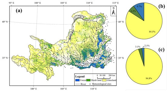
Figure 1.
Location and land cover of the Yellow River Basin. (a) Location, river, meteorological sites, and land-cover types of the study region in 2015 from CESA land-cover map. (b) Area proportion of grassland, forest, and shrub land converted from farmland in the period of 1990 to 2015. (c) The area proportion of grassland, forest, and shrub land converted from bare land in the period of 1990 to 2015.
2.2. Data Collection
2.2.1. NPP Data
NPP (gC·m−2·yr−1) data were collected from NASA Moderate Resolution Imagine Spectroradiometer (MODIS) MOD17 NPP products, while the production is determined by first computing a daily net photosynthesis (PSN) value, which is then composited over an 8-day interval of observations for a day. The product is wildly used in calculating terrestrial energy, carbon, water cycle process, and biogeochemistry of vegetation [40,41,42]. This study used 2016–2020 annual NPP data extracted from MOD17A3HGF v006 based on the sum of all 8-day PSN products from the given year at a 500 m spatial resolution (https://lpdaac.usgs.gov/products/mod17a3hgfv006, accessed on 10 October 2021).
2.2.2. Climate Data
Climate data from 376 weather stations distributed across the YRB were retrieved from the China Meteorological Data Sharing Network (http://data.cma.cn, accessed on 5 October 2021). Collected data contain daily and annual average temperature (AT, °C), daily and annual precipitation (AP, mm), average daily wind speed (m·s−1), daily radiation(MJ·m−2·day−1), and daily sunshine duration(h) from 2016 to 2020. The daily potential evapotranspiration (ETP, mm/d) was calculated by daily meteorological observation data with the Penman-Monteith equation as follows
where was the slop of saturation vapor pressure curve (kPa·°C) at air temperature, Rn is the net daily radiation at the vegetated surface (MJ·m−2·day−1), G is the soil heat flux (MJ·m−2·day−1), is the psychrometric constant (kPa·°C), Tavg is the mean daily air temperature (°C) at 2 m height, is the average daily wind speed (m·s−1) at 2 m height and is the vapor pressure deficit (kPa).
The arid index (AI) was used to indicate the water available condition [43], which was calculated as follows
where METP was the mean annual potential evapotranspiration (mm/yr), which was calculated as the annual average of ETP, and MAP is the mean annual precipitation. In the semi-arid area AI < 3 while in the arid area AI > 3.
To identify a spatial pattern in climatic parameters, we used the ANUSPLINA4.3 package to interpolate climate data into a 500 m spatial solution with a thin plate smoothing splines algorithm. ANNUSPLINA4.3 package is a widely used measure for interpolating time series meteorological data with a high-definition [44,45].
2.2.3. Land Cover Data
The land cover maps of YRB were collected from the national ecosystem survey and assessment of China (CESA) with a 30 m spatial resolution, which covers four time points (1990, 2000, 2010, and 2015). CESA land cover maps were produced by using Landsat Thematic Mapper (TM) and Enhanced Thematic Mapper (ETM) images and domestic HJ-1 images verified by 675 field surveys [46]. Using 2015 land-cover data, we show the distribution of grassland, shrub land, and forest and in YRB in Figure 1a. Grassland, forest, and shrub land cover 46.2%, 7.2%, and 11.8% area of YRB, respectively. Forests and shrubs mostly grow in the southeast and grasslands mostly grow in the west and northwest area of YRB. By comparing the 1990 (before “Grain-for-Green” and other ecological restoration programs were implemented) and 2015 CESA land cover maps, we identified the original grassland, shrub land, and forest that remained the same between 1990 and 2015, while artificial vegetation was identified as farmland or bare land in 1990 but had been converted to grassland, shrub land and forest in 2015. CESA land-cover data were resampled into 500 m spatial resolution by Arcgis 10.5.
2.3. Data Calculate and Analysis
2.3.1. PUE Calculate
PUE (gC·m−2·mm−1) was calculated at each 500 m raster as the ratio of NPP to AP [47]:
Because AP, AT, NPP, and PUE fluctuated annually and changed significantly over the past two decades, here we calculated the average of 2001–2020 AP and AT as MAP and MAT, calculated 2016–2020 average NPP and PUE to explore spatial heterogeneity.
2.3.2. Statistical Analysis
To describe the fluctuation intensity of NPP, PUE, AP, and AT in spatial statistics, we used the coefficient of variation (CV):
where n is the time-series number or the spatial-series number and y is NPP, PUE, AP, and AT.
According to the 2015 CESE land-cover map, NPP, PUE, and their mean value of grassland, shrub land, and forest were classified. To explore spatial patterns of NPP and PUE along geographic and climate gradients, we calculated the mean value of NPP and PUE at 1° intervals in latitude, 1° intervals in longitude, 100 m intervals in elevation, 50 mm intervals in MAP, 1 °C intervals in MAT and 0.5-unit intervals in AI. The correlation of NPP and PUE with geographic, climate factors was obtained using Origin 2021b software through polynomial fitting and significance analysis.
To estimate the effect intensity of geographical factors and climate factors that control the spatial pattern of NPP and PUE, we performed structural equation models (SEM). SEM technique represents linear relationships between variables in a theoretical network and is widely used to analyze the relationship between variables in the biophysical systems [48,49]. A cascading effect existed whereby geographical factors (Longitude, Latitude, and Altitude) directly affected climate factors (MAT, MAP, and AI), which in turn led to spatial heterogeneity in NPP and PUE. The structural equation models were performed by SPSSAU at http://www.spssau.com (accessed on 3 November 2021).
The data processing steps and methodology applied in this study was shown in Figure 2.
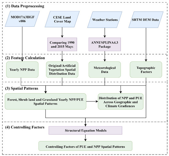
Figure 2.
The flowchart of the data processing steps and methodology applied in this study.
3. Results
3.1. Spatial Heterogeneity of PUE and NPP
In YRB, NPP and PUE variation trends were roughly the same and decreased from southeast to northwest (Figure 3a,b), differing significantly between 27.59–1043.36 gC·m−2·yr−1 and 0.06–3.30 gC·m−1·mm−1, respectively. Figure Southeast mountains and plains deciduous broadleaf forest and deciduous broadleaf shrub land had the highest values of NPP that exceeded 539.63 gC·m−2·yr−1, where PUE exceeded 0.85 gC·m−1·mm−1. Northwest and west region temperate steppe and alpine steppe had the lowest values of NPP that less than 155.46 gC·m−2·yr−1 and the lowest values of PUE that less than 0.28 gC·m−1·mm−1.
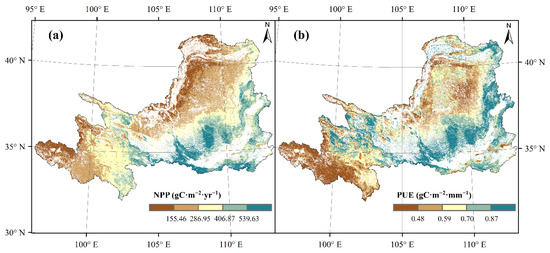
Figure 3.
Spatial patterns of (a) NPP and (b) PUE of forest, shrub land and grassland across the YRB.
In terms of different vegetation types(Table 1), the forest had the highest NPP (avg = 488.26 gC·m−2·yr−1), PUE (avg = 0.82 gC·m−1·mm−1), and MAP (609.07 mm) values, followed by shrub land with medium values, while lowest values were calculated for grassland NPP, PUE, and MAP. However, grassland had the highest CVNPP (39.54%) and CVPUE (31.72%), indicating that grassland had the highest NPP and PUE spatial heterogeneity. Shrub land had the medium CVNPP (32.81%) and CVPUEue (25.94%) while forest had the lowest CVNPP (25.11%) and CVPUE (24.15%). In summary, forest, which generally grows in moist environments, had the greatest capacity to produce organic matter with the highest precipitation-use efficiency, whereas grassland was the opposite, and shrub land was in the middle.

Table 1.
The spatial mean, maximum, minimum, coefficient of variation(CV) of the forest, shrub land, grassland NPP and PUE, and the spatial average MAP(MAPavg) in their respective distribution areas.
3.2. Distribution of NPP and PUE across Geographic and Climate Gradiences
The spatial variations of NPP and PUE in the YRB exhibited strong correlations with geographical and climatic factors. Forest and shrub land NPP showed increase-decrease patterns across latitude (R2 = 0.86, 0.83, p < 0.01), longitude (R2 = 0.79, 0.88, p < 0.01), and elevation gradients (R2 = 0.98, 0.95, p < 0.01). Higher NPP values were appeared around 34°N, 107°E and at the elevation of 2000 m. The NPP patterns of grassland, however, were shown to be more gradual and with lower values. They differed from those of forest and shrub land in terms of their variation patterns and position of the largest NPP value (Figure 4a–c). The PUE patterns of forest, shrub land, and grassland were generally consistent with the NPP patterns of each type of plant. Grasslands also had a lower PUE compared to forest and shrub land with slightly different patterns spatially, even though PUE fluctuated across latitude, longitude, and elevation regardless of the plant type (Figure 4d–f).
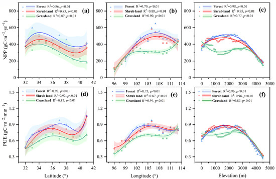
Figure 4.
Variations in NPP and PUE across latitude (a,d), longitude (b,e), and elevation (c,f) gradient of forest, shrub land and grassland in the YRB. Soild lines are the regression curves, and shading represented the regression analysis confidence range (5th and 95th percentiles). Each point is the bin-averaged value at 1° latitude intervals in (a,d), 1° longitude intervals in (b,e) and 100 m elevation intervals in (c,f).
For forest, shrub land and grassland, the mean NPP values displayed significant positive linear patterns across the gradient of MAP (R2 = 0.84, 0.91, 0.92, respectively) (Figure 5a). The NPP of forest, shrub landshrub land and grassland increased 64.16 gC·m−2·yr−1, 73.09 gC·m−2·yr−1 and 84.80 gC·m−2·yr−1 after every 100 mm increase in MAP, respectively. On the contrary, NPP displayed significant negative linear patterns across the gradient of AI (forest: R2 = 0.94, shrub land: R2 = 0.97, grassland: R2 = 0.98, respectively) (Figure 5c). The NPP of forest, shrub landshrub land and grassland decreased 112.52 gC·m−2·yr−1, 94.95 gC·m−2·yr−1 and 60.75 gC·m−2·yr−1 for every one unit increase in AI, respectively. The patterns of NPP across MAT gradient varied among different vegetation types. The NPP of forest and shrub land was positive correlated with MAT where MAT < 0 °C and exhibited stable where MAT > 0 °C (R2 = 0.97, 0.96, respectively) (Figure 4b), but for grassland, the relationship between grassland NPP and MAT was choppy (R2 = 0.99) (Figure 5b).
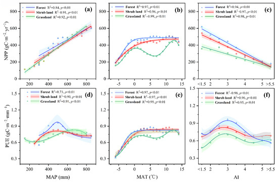
Figure 5.
Variations in NPP and PUE across the map (a,d), MAT (b,e), and AI (c,f) gradient of the forest, shrub land, and grassland in the YRB. Lines were the regression curves, and shading represented the regression analysis confidence range (5th and 95th percentiles). Each point was the averaged value at 50 mm MAP intervals in (a,d), 1 °C MAT intervals in (b,e), and 0.5-unit AI intervals in (c,f).
There appeared to be segmented trends in PUE related to MAP and AI. For the grassland, PUE decreased where MAP < 350 mm, increased where 300 < MAP < 600 mm and decreased where MAP > 600 mm. For the forest and shrub landshrub land, PUE exhibited increase-decrease trend while increased where MAP < 500 mm and decreased where MAP > 500 mm (forest: R2 = 0.73, shrub land: R2 = 0.90, grassland: R2 = 0.91, respectively) (Figure 5d). AI = 3 was the turning point of PUE’s increase-decrease trend across AI gradient for all vegetation types (forest: R2 = 0.98, shrub landshrub land: R2 = 0.96, grassland: R2 = 0.95, respectively) (Figure 5f). The relationship between PUE and MAT of each type of vegetation was like to that of NPP and MAT, which showed piecewise patterns in forest and shrub land with turning point at 0 °C, after which NPP and PUE followed a straight-line trend and choppy pattern for grassland (forest: R2 = 0.97, shrub land: R2 = 0.97 grassland: R2 = 0.99, respectively) (Figure 5e)).
3.3. Controlling Factors of PUE and NPP Spatial Patterns
Based on SEM, geographical and climate factors accounted for their in-cascading effects on NPP and PUE, and results indicated that geographic factors governed MAT, MAP, and AI, further affecting NPP and PUE. For all vegetation in YRB, climate factors (MAT, MAP, and AI) account for 56% and 93% of the spatial variation in NPP and PUE, respectively, while geographic factors (latitude, longitude, and elevation) contributed 98%, 59% and 62% of the variation in MAT, MAP, and AI, respectively (Figure 6d).
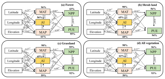
Figure 6.
SEMs of geographic factors (Latitude, longitude, and elevation) and climate factors (MAP, MAT, and AI) on spatial variation of NPP and PUE for forest (a), shrub land (b), grassland (c), and all vegetation (d). Solid and dashed arrows represented the positive or negative effects in fitted SEMs, respectively. The * and ** represented a significant relationship at p < 0.05 and p < 0.01, respectively.
MAT and MAP both had the opposite impact on NPP (positive, p < 0.01) and PUE (negative, p < 0.01) of shrub land and grassland, while MAT had a negative effect on forest NPP as well as PUE (p < 0.01). AI showed negative relationships with NPP and PUE of all kinds of vegetation (p < 0.01). Meanwhile, AI was the major controlling factor of the NPP spatial pattern with a correlation coefficient of −0.45 (p < 0.01), despite MAT and MAP being positively correlated with correlation coefficient values of 0.37 and 0.39, respectively. On the other hand, PUE was influenced mainly by MAP (−0.85, p < 0.01) and NPP (0.82, p < 0.01). it is also important to mention that, The NPP of grassland was more sensitive to the spatial pattern of MAT (0.41) and MAP (0.43), compared to the forest (−0.08, 0.27) and shrub land (0.16, 0.42). Despite wide correlations between climate factors, the PUE of each vegetation type was primarily controlled by their NPP (0.89 in forest, 0.84 in shrub land and 0.80 in grassland).
4. Discussion
4.1. Spatial Pattern Characteristics of NPP and PUE
We provided a detailed picture of the NPP and PUE patterns in the YRB, which are influenced by the various landforms, the largely changed topography, the diversified climate, and the regional particularities of plants. Our results indicated that the spatial variation trends for NPP and PUE were broadly consistent in YRB, decreasing from southeast to northwest. Both NPP and PUE varied nonlinearly across latitude, longitude, and elevation in YRB, in contrast to Eurasian grasslands [17], North-South Transect forests of China [50], and China’s grasslands [21]. NPP and PUE values varied from 27.59 to 1043.36 gC·m−1·mm−1 and from 0.06 to 3.25 gC·m−1·mm−1, with the mean values of 358.18 gC·m−1·mm−1 and 0.72 gC·m−1·mm−1, respectively. In previous studies, NPP and PUE values that were measured by field survey and flux observation in YRB varied from 70.49 to 956.72 gC·m−1·mm−1 and from 0.17 to 1.71 gC·m−1·mm−1, with the mean values of 331.06 gC·m−1·mm−1 and 0.74 gC·m−1·mm−1, respectively [17,20,51,52,53,54]. Since remote sensing NPP is credible and convenient, it is feasible to estimate vegetation productivity and precipitation use efficiency
Compared with grassland and shrub land, the forest had the highest mean NPP value and the lowest CVNPP in YRB, indicating that the forest had the highest and most stable productivity. In addition, the forest had a higher and more stable mean PUE than grassland and shrub land, which means that it had a more effective water use strategy. It could be attributed to the fact that most of the forests were located in moist regions with MAP > 400 mm and AI < 3, as well as their higher plant species richness, which had been demonstrated to enhance water use efficiency at the community scale [55,56,57,58]. This may be attributed to the notion that more species may result in more efficient use of precipitation due to niche complementarity, while higher species richness can lead to more functional groups that are responsive to higher precipitation levels [11,59,60]. On the contrary, growing in drier regions has poor plant species richness, that is why grassland had the lowest and most variable NPP and PUE values.
It seems that due to the unique geographic conditions and the complex interactions between physical water cycles and plant physiology, local-specific variations of NPP and PUE are prevalent [22]. Previous studies reported that NPP increased with MAP gradient, especially in arid and semiarid ecosystems where precipitation plays a vital role in replenishing soil moisture [10,20,50]. In our analysis, we calculated the mean NPP over 50 mm MAP intervals for each vegetation type and found that NPP correlated linearly with MAP, like in the previous research [61,62].
However, the positive linear correlation of MAP-NPP did not result in a relatively constant PUE in YRB, PUE appeared to be segmented trends along MAP gradient, similar to the research of global grassland [63]. It may be because our PUE was calculated directly from NPP to AP ratios and averaged over MAP gradient, rather than obtained by calculating the MAP-PUE spatial relationship (slope, for example) [10]. However, our finding that PUE exhibited a segmented pattern across the precipitation gradient in YRB, which was inconsistent with some previous studies, such as a linear positive pattern found in a 4500-km grassland transect [10] and a linear negative pattern found in a Chinese warm temperate deciduous broad-leaved forest [50] but similar to the unimodal pattern observed in Northern Tibet grassland [64]. Wetter sites tend to have lower PUE because excessive precipitation exceeds vegetation needs, while drier sites tend to have lower PUE due to low plant density, low production potential, high evaporation potential, and high tolerance to water stress [65,66,67]. Meanwhile, the segmented correlation of MAP-PUE varied between vegetation types, the peak of the grassland MAP-PUE curve appeared at a higher MAP (700 mm) than that of forest (500 mm) and shrub land (500 mm), while the forest’s curve had a higher peak (0.96 gC·m−1·mm−1) than shrub land (0.84 gC·m−1·mm−1) and grassland (0.83 gC·m−1·mm−1). Ecosystem complexity and different water use strategies may be responsible for this difference between vegetation types [9,16].
4.2. Hydrothermal Controlling Mechanism of NPP and PUE Spatial Patterns
Based on our findings, MAP, MAT, and AI were strongly influenced by geographic factors and played a significant role in controlling the spatial variations of NPP and PUE in the Yellow River Basin, consistent with the previous finding of Eurasian grasslands [17] and three typical revegetation species on the Loess Plateau [68]. As a typical semi-arid and arid area, water condition was the primary factor that controlled the spatial patterns of NPP and PUE. MAP had opposite effects on NPP and PUE, positively affecting NPP but negatively affecting PUE. However, AI played a more critical role in controlling NPP spatial patterns than MAP, suggesting that vegetation productivity was more dependent on available water than total precipitation. Higher AI indicates a lower ratio between annual precipitation and evapotranspiration, indicating a dry climate. Moreover, AI was significantly correlated with precipitation stability, as well as water availability in the plant, which constrained the photosynthetic production [21,23,69].
According to previous studies, YRB is likely to become more arid in the future with less precipitation and higher temperatures [6,70]. As AI was associated with both water and heat, MAT, and MAP controlled vegetation production differently along AI gradients. Based on the Person correlation, we calculated the correlation between MAP, MAT, and NPP of original vegetation and artificial vegetation, R2 was used to represent the coefficient of determination. The result showed an increasing control of MAP with increasing AI (more arid), but a decreasing control of MAT, indicating that, in the wetter area, vegetation product was mainly controlled by heat because the water was plentiful, but in drier area, moisture was a more important control of plant productivity since the water was scarce.
The threshold point at which MAT-controlling NPP turned into MAP-controlling varied with vegetation type. For grassland, it occurred when AI was about 4, with drier conditions than for shrub land and forest (Figure 7c–h), suggesting that grassland was mainly controlled by MAT in more area than other plant types. The reason could be that 21.33% of grassland in YRB comprised alpine steppe and alpine meadows, the growth of which is significantly affected by temperature [69,71]. Moreover, artificial grassland, which was widely distributed in the medium area, particularly the Loess plateau and alpine region, its threshold point appeared in even more arid condition than that of the original grassland (Figure 7c,f). By comparison, artificial shrub land had a threshold point that was almost identical to that of the original shrub land (Figure 7d,g). The correlation counted by remote data along AI gradients did not appear to be significant for forest land, because forest covered only 7.817% of the YRB and the majority of it is located in the southeast where AI was less than 3, and artificial forest made up only 2.17% of the total forest and covered less than 10% of the artificial vegetation area (Figure 1b,c). Hence, the hydrothermal controlling mechanism of forest NPP spatial pattern requires further investigation.
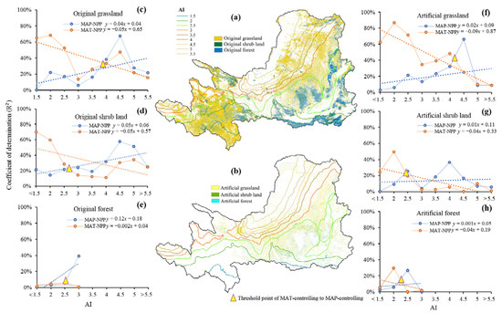
Figure 7.
AI gradients with (a) original vegetation distribution and (b) artificial vegetation distribution, and correlation coefficient of determination (R2) among MAT, MAP, and NPP along AI gradients in (c) original grassland, (d) original shrub land, (e) original forest, (f) artificial grassland, (g) artificial shrub land, and (h) artificial forest.
4.3. Implication for Revegetation and Land Management
The distribution of original vegetation at the basin scale was regional, as a result of climate conditions linked to moisture and heat [72]. As that climate condition becomes more arid in the future, vegetation will become more sensitive to moisture in YRB [6]. Since that 66,100 km2 of farmland and 2093 km2 of bare land had converted into artificial vegetation (forest, shrub land, and grassland), and their suitability to YRB has been through different methods based on diversified plant types [73], some typical artificial plants, such as Robinia pseudoacacia, had significantly smaller plants than in other area [36].
It is noteworthy that compared to original vegetation, artificial forest, artificial shrub land, and artificial grassland converted from bare land and farmland had lower NPP and PUE (Figure 8a,b). Perhaps this happen because low productivity farmland which was already facing serious water and soil erosion was converted to artificial farmland under the Grain for Green program [39,74]. Therefore, restoration vegetation planted in abandoned slope farmland may be restricted to water and nutrients because of soil erosion, creating new uncertainties for the ecosystem, further affecting NPP and PUE [6,75]. With regard to bare land that is converted into vegetation, revegetation increased evapotranspiration (ET) and depleted soil moisture, intensifying the water competition in the ecosystem, resulting in adverse effects on plant growth and water storage [5,76].
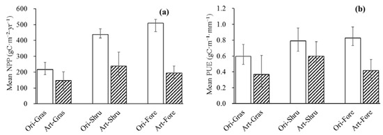
Figure 8.
The mean NPP (a) and PUE (b) of original vegetation and artificial vegetation. Ori-Gras, Art-Gras, Ori-Shru, Art-Shru, Ori-Fore, and Art-For represented original grassland, artificial grassland, original shrub land, artificial shrub land, original forest and artificial forest, respectively. Error bar represented the standard deviation (SD).
Furthermore, excessive vegetation water consumption overburdened water resources in the basin [77,78], the NPP created by vegetation in the watershed has already been overloaded, which brought prominent competition between human and vegetation water use and threatened water security [1,79]. There have been extensive studies on the appropriate plant species for restoration and the applicability of existing plantings in this area, the consensus was that continuous desiccation of the climate in the future will further reduce the suitability range of artificial vegetation, especially artificial forests [6,68,73]. This prediction could be explained further by our findings regarding MAP and MAT controlling mechanisms for NPP. As a result of climate change the entire basin will become arid with higher AI values, which means the NPP of all plants will decrease and more vegetation will shift from MAT-controlling to MAP-controlling. It follows that increased sensitivity of vegetation to water availability will contribute to reduced tolerance to water variations, as well as an increase in conflict between vegetation and human society regarding water availability. The loss of vegetation productivity and increased water insecurity is clearly counterproductive to the original intentions of ecological restoration; thus, drought-tolerant, and stable carbon sequestration plants for wind prevention and sand fixing will be preferable to plants that require a lot of water. Consequently, it encourages us to think seriously about how to restore the vegetation of the Yellow River Basin so that both economic and ecological benefits can be achieved parallelly.
5. Conclusions
We studied the spatial pattern and biogeographic mechanism of NPP and PUE in YRB to determine whether ecological restoration programs are effective at restoring ecosystem function under climate change. Here we integrated remote sensing observation with in-situ climate data to estimate NPP and PUE value at the basin scale and for each vegetation type (forest, shrub land, and grassland) separately. Findings of this study reveal that NPP and PUE spatial trends were consistent along the geographical gradients. Forest was the most productive ecosystem with the highest mean NPP and PUE with the lowest CVNPP and CVPUE, and grassland with the lowest NPP and PUE values. NPP and PUE showed segmented patterns across geographical (latitude, longitude, and elevation) gradients and MAT gradients. NPP displayed significant positive linear patterns across MAP but negative linear patterns across AI, while PUE showed segmented trends with MAP and AI.
We used SEMs to affirm how geographic factors influence MAP, MAT, and AI, further affecting NPP and PUE by following a cascading effect. SEMs revealed that NPP was mainly controlled by AI, while PUE was mainly controlled by NPP and MAP. The hydrothermal controlling mechanism of the NPP spatial pattern indicated that the main controlling climate factor of NPP changed from MAT to MAP with AI increasing. Grassland was more sensitive to MAT than forest and shrub land with the threshold point appearing in drier conditions. In view of the upcoming higher AI in the further, NPP across YRB will decrease and vegetation will become more sensitive to water availability. Artificial vegetation exhibited lower NPP and PUE than original vegetation since it had already caused a variety of ecological problems, especially increased water competition between human society and the ecosystem, drought-tolerant and stable carbon sequestration plants for wind prevention and sand fixing will be preferable in ecological restoration to plants that require a lot of water. These results have improved our understanding of regional patterns and biogeographic processes of NPP and PUE across YRB, allowing us to optimize the spatial structure of vegetation.
Author Contributions
Y.L. guided the paper writing and adjusted the structure; T.J. collected the data, analyzed the result, and wrote the original draft; L.S. investigated data and performed data analyses; X.W. provided suggestions and revised the paper; M.M.A. provided suggestions and revised the paper. All authors have read and agreed to the published version of the manuscript.
Funding
This study was supported by the Strategic Priority Research Program of the Chinese Academy of Sciences, Pan-Third Pole Environment Study for a Green Silk Road (XDA20060301) and the National Key Research and Development Program (2016YFC0501603).
Conflicts of Interest
The authors declare no conflict of interest.
References
- Feng, X.; Fu, B.; Piao, S.; Wang, S.; Ciais, P.; Zeng, Z.; Lü, Y.; Zeng, Y.; Li, Y.; Jiang, X.; et al. Revegetation in China’s Loess Plateau is approaching sustainable water resource limits. Nat. Clim. Chang. 2016, 6, 1019–1022. [Google Scholar] [CrossRef]
- Li, H.; Luo, Y.; Sun, L.; Li, X.; Ma, C.; Wang, X.; Jiang, T.; Zhu, H. Modelling the artificial forest (Robinia pseudoacacia L.) root-soil water interactions in the Loess Plateau, China. Hydrol. Earth Syst. Sci. 2022, 26, 17–34. [Google Scholar] [CrossRef]
- Li, S.; Liang, W.; Fu, B.; Lu, Y.; Fu, S.; Wang, S.; Su, H. Vegetation changes in recent large-scale ecological restoration projects and subsequent impact on water resources in China’s Loess Plateau. Sci. Total Environ. 2016, 569–570, 1032–1039. [Google Scholar] [CrossRef]
- Su, C.; Fu, B. Evolution of ecosystem services in the Chinese Loess Plateau under climatic and land use changes. Glob. Planet. Chang. 2013, 101, 119–128. [Google Scholar] [CrossRef]
- Zhao, M.; Geruo, A.; Zhang, J.; Velicogna, I.; Liang, C.; Li, Z. Ecological restoration impact on total terrestrial water storage. Nat. Sustain. 2020, 4, 56–62. [Google Scholar] [CrossRef]
- Wang, C.; Wang, S.; Fu, B.; Lu, Y.; Liu, Y.; Wu, X. Integrating vegetation suitability in sustainable revegetation for the Loess Plateau, China. Sci. Total Environ. 2021, 759, 143572. [Google Scholar] [CrossRef]
- Meier, R.; Schwaab, J.; Seneviratne, S.I.; Sprenger, M.; Lewis, E.; Davin, E.L. Empirical estimate of forestation-induced precipitation changes in Europe. Nat. Geosci. 2021, 14, 473–478. [Google Scholar] [CrossRef]
- Peng, S.S.; Piao, S.; Zeng, Z.; Ciais, P.; Zhou, L.; Li, L.Z.X.; Myneni, R.B.; Yin, Y.; Zeng, H. Afforestation in China cools local land surface temperature. Proc. Natl. Acad. Sci. USA 2014, 111, 2915–2919. [Google Scholar] [CrossRef]
- Zhu, Y.; Delgado-Baquerizo, M.; Shan, D.; Yang, X.; Liu, Y.; Eldridge, D.J. Diversity-productivity relationships vary in response to increasing land-use intensity. Plant Soil. 2020, 450, 511–520. [Google Scholar] [CrossRef]
- Hu, Z.; Yu, G.; Fan, J.; Zhong, H.; Wang, S.; Li, S. Precipitation-use efficiency along a 4500-km grassland transect. Glob. Ecol. Biogeogr. 2010, 19, 842–851. [Google Scholar] [CrossRef]
- Hooper, D.U.; Chapin, F.S.; Ewel, J.J.; Hector, A.; Inchausti, P.; Lavorel, S.; Lawton, J.H.; Lodge, D.M.; Loreau, M.; Naeem, S.; et al. Effects of biodiversity on ecosystem functioning: A consensus of current knowledge. Ecol. Monogr. 2005, 75, 3–35. [Google Scholar] [CrossRef]
- McNaughton, S.J.; Oesterheld, M.; Frank, D.A.; Williams, K.J. Ecosystem-level patterns of primary productivity and herbivory in terrestrial habitats. Nature 1989, 341, 142–144. [Google Scholar] [CrossRef] [PubMed]
- Roy, J.; Saugier, B.; Mooney, H.A. Terrestrial Global Productivity; Academic Press: Cambridge, MA, USA, 2001. [Google Scholar]
- Wang, Y.; Sun, J.; Liu, M.; Zeng, T.; Tsunekawa, A.; Mubarak, A.A.; Zhou, H. Precipitation-use efficiency may explain net primary productivity allocation under different precipitation conditions across global grassland ecosystems. Glob. Ecol. Conserv. 2019, 20, e00713. [Google Scholar] [CrossRef]
- Huxman, T.E.; Smith, M.D.; Fay, P.A.; Knapp, A.K.; Shaw, M.R.; Loik, M.E.; Smith, S.D.; Tissue, D.T.; Zak, J.C.; Weltzin, J.F.; et al. Convergence across biomes to a common rain-use efficiency. Nature 2004, 429, 651–654. [Google Scholar] [CrossRef]
- Knapp, A.K.; Ciais, P.; Smith, M.D. Reconciling inconsistencies in precipitation–productivity relationships: Implications for climate change. New Phytol. 2016, 214, 41–47. [Google Scholar] [CrossRef]
- Zhang, T.; Yu, G.; Chen, Z.; Hu, Z.; Jiao, C.; Yang, M.; Fu, Z.; Zhang, W.; Han, L.; Fan, M.; et al. Patterns and controls of vegetation productivity and precipitation-use efficiency across Eurasian grasslands. Sci. Total Environ. 2020, 741, 140204. [Google Scholar] [CrossRef]
- Peng, Z.; Wang, L.; Xie, J.; Li, L.; Coulter, J.A.; Zhang, R.; Luo, Z.; Cai, L.; Carberry, P.; Whitbread, A. Conservation tillage increases yield and precipitation use efficiency of wheat on the semi-arid Loess Plateau of China. Agric. Water Manag. 2020, 231, 106024. [Google Scholar] [CrossRef]
- Ponce-Campos, G.E.; Moran, M.S.; Huete, A.; Zhang, Y.; Bresloff, C.; Huxman, T.E.; Eamus, D.; Bosch, D.D.; Buda, A.R.; Gunter, S.A.; et al. Ecosystem resilience despite large-scale altered hydroclimatic conditions. Nature 2013, 494, 349–352. [Google Scholar] [CrossRef]
- Jia, X.X.; Xie, B.N.; Shao, M.; Zhao, C.L. Primary Productivity and Precipitation-Use Efficiency in Temperate Grassland in the Loess Plateau of China. PLoS ONE 2015, 10, e0135490. [Google Scholar] [CrossRef]
- Sun, J.; Du, W. Effects of precipitation and temperature on net primary productivity and precipitation use efficiency across China’s grasslands. GIScience Remote Sens. 2017, 54, 881–897. [Google Scholar] [CrossRef]
- Yang, Z.; Collins, S.L.; Bixby, R.J.; Song, H.; Wang, D.; Xiao, R. A meta-analysis of primary productivity and rain use efficiency in terrestrial grassland ecosystems. Land Degrad. Dev. 2020, 32, 842–850. [Google Scholar] [CrossRef]
- Zhang, J.; Li, J.; Xiao, R.; Zhang, J.; Wang, D.; Miao, R.; Song, H.; Liu, Y.; Yang, Z.; Liu, M.; et al. The response of productivity and its sensitivity to changes in precipitation: A meta-analysis of field manipulation experiments. J. Veg. Sci. 2020, 32, e12954. [Google Scholar] [CrossRef]
- Fu, B.; Wang, S.; Liu, Y.; Liu, J.; Liang, W.; Miao, C. Hydrogeomorphic Ecosystem Responses to Natural and Anthropogenic Changes in the Loess Plateau of China. Annu. Rev. Earth Planet. Sci. 2017, 45, 223–243. [Google Scholar] [CrossRef]
- Tang, Q.; Oki, T.; Kanae, S.; Hu, H. A spatial analysis of hydro-climatic and vegetation condition trends in the Yellow River basin. Hydrol. Process. 2008, 22, 451–458. [Google Scholar] [CrossRef]
- Sun, Q.; Miao, C.; Duan, Q.; Wang, Y. Temperature and precipitation changes over the Loess Plateau between 1961 and 2011, based on high-density gauge observations. Glob. Planet. Chang. 2015, 132, 1–10. [Google Scholar] [CrossRef]
- Wang, Q.-X.; Fan, X.-H.; Qin, Z.-D.; Wang, M.-B. Change trends of temperature and precipitation in the Loess Plateau Region of China, 1961–2010. Glob. Planet. Chang. 2012, 92–93, 138–147. [Google Scholar] [CrossRef]
- Li, Z.; Liu, W.-Z.; Zhang, X.-C.; Zheng, F.-L. Assessing the site-specific impacts of climate change on hydrology, soil erosion and crop yields in the Loess Plateau of China. Clim. Chang. 2011, 105, 223–242. [Google Scholar] [CrossRef]
- Yuan, M.; Wang, L.; Lin, A.; Liu, Z.; Li, Q.; Qu, S. Vegetation green up under the influence of daily minimum temperature and urbanization in the Yellow River Basin, China. Ecol. Indic. 2020, 108, 105760. [Google Scholar] [CrossRef]
- Bryan, B.A.; Gao, L.; Ye, Y.; Sun, X.; Connor, J.D.; Crossman, N.D.; Stafford-Smith, M.; Wu, J.; He, C.; Yu, D.; et al. China’s response to a national land-system sustainability emergency. Nature 2018, 559, 193–204. [Google Scholar] [CrossRef]
- Feng, X.; Fu, B.; Lu, N.; Zeng, Y.; Wu, B. How ecological restoration alters ecosystem services: An analysis of carbon sequestration in China’s Loess Plateau. Sci. Rep. 2013, 3, 2846. [Google Scholar] [CrossRef]
- Zhu, Z.; Piao, S.; Myneni, R.B.; Huang, M.; Zeng, Z.; Canadell, J.G.; Ciais, P.; Sitch, S.; Friedlingstein, P.; Arneth, A.; et al. Greening of the Earth and its drivers. Nat. Clim. Chang. 2016, 6, 791–795. [Google Scholar] [CrossRef]
- Wang, S.; Fu, B.; Piao, S.; Lü, Y.; Ciais, P.; Feng, X.; Wang, Y. Reduced sediment transport in the Yellow River due to anthropogenic changes. Nat. Geosci. 2015, 9, 38–41. [Google Scholar] [CrossRef]
- Chen, C.; Park, T.; Wang, X.; Piao, S.; Xu, B.; Chaturvedi, R.K.; Fuchs, R.; Brovkin, V.; Ciais, P.; Fensholt, R.; et al. China and India lead in greening of the world through land-use management. Nat. Sustain. 2019, 2, 122–129. [Google Scholar] [CrossRef] [PubMed]
- Zhang, X.; Zhang, L.; Zhao, J.; Rustomji, P.; Hairsine, P. Responses of streamflow to changes in climate and land use/cover in the Loess Plateau, China. Water Resour. Res. 2008, 44. [Google Scholar] [CrossRef]
- Jia, X.; Shao, M.; Zhu, Y.; Luo, Y. Soil moisture decline due to afforestation across the Loess Plateau, China. J. Hydrol. 2017, 546, 113–122. [Google Scholar] [CrossRef]
- Jiang, W.; Yuan, L.; Wang, W.; Cao, R.; Zhang, Y.; Shen, W. Spatio-temporal analysis of vegetation variation in the Yellow River Basin. Ecol. Indic. 2015, 51, 117–126. [Google Scholar] [CrossRef]
- Cao, Z.; Li, Y.; Liu, Y.; Chen, Y.; Wang, Y. When and where did the Loess Plateau turn “green”? Analysis of the tendency and breakpoints of the normalized difference vegetation index. Land Degrad. Dev. 2018, 29, 162–175. [Google Scholar] [CrossRef]
- Yu, Y.; Zhao, W.; Martinez-Murillo, J.F.; Pereira, P. Loess Plateau: From degradation to restoration. Sci. Total Environ. 2020, 738, 140206. [Google Scholar] [CrossRef]
- Park, J.H.; Gan, J.; Park, C. Discrepancies between Global Forest Net Primary Productivity Estimates Derived from MODIS and Forest Inventory Data and Underlying Factors. Remote Sens. 2021, 13, 1441. [Google Scholar] [CrossRef]
- Zhao, Y.; Liu, H.; Zhang, A.; Cui, X.; Zhao, A. Spatiotemporal variations and its influencing factors of grassland net primary productivity in Inner Mongolia, China during the period 2000–2014. J. Arid Environ. 2019, 165, 106–118. [Google Scholar] [CrossRef]
- de Leeuw, J.; Rizayeva, A.; Namazov, E.; Bayramov, E.; Marshall, M.T.; Etzold, J.; Neudert, R. Application of the MODIS MOD 17 Net Primary Production product in grassland carrying capacity assessment. Int. J. Appl. Earth Obs. Geoinf. 2019, 78, 66–76. [Google Scholar] [CrossRef]
- Huang, J.; Yu, H.; Guan, X.; Wang, G.; Guo, R. Accelerated dryland expansion under climate change. Nat. Clim. Chang. 2015, 6, 166–171. [Google Scholar] [CrossRef]
- Hijmans, R.J.; Cameron, S.E.; Parra, J.L.; Jones, P.G.; Jarvis, A. Very high resolution interpolated climate surfaces for global land areas. Int. J. Climatol. 2005, 25, 1965–1978. [Google Scholar] [CrossRef]
- McVicar, T.R.; Van Niel, T.G.; Li, L.; Hutchinson, M.F.; Mu, X.; Liu, Z. Spatially distributing monthly reference evapotranspiration and pan evaporation considering topographic influences. J. Hydrol. 2007, 338, 196–220. [Google Scholar] [CrossRef]
- Wu, B.; Qian, J.; Zeng, Y.; Zhang, L.; Yan, C.; Wang, Z.; Li, A.; Ma, R.; Yu, X.; Huang, J. Land Cover Atlas of the People’s Republic of China (1: 1,000,000); China Map Publishing House: Beijing, China, 2017. [Google Scholar]
- Le Houérou, H.; Bingham, R.; Skerbek, W. Relationship between the variability of primary production and the variability of annual precipitation in world arid lands. J. Arid Environ. 1988, 15, 1–18. [Google Scholar] [CrossRef]
- Anderson, J.C.; Gerbing, D.W. Structural Equation Modeling In Practice—A Review And Recommended 2-Step Approach. Psychol. Bull. 1988, 103, 411–423. [Google Scholar] [CrossRef]
- Tedersoo, L.; Bahram, M.; Põlme, S.; Kõljalg, U.; Yorou, N.S.; Wijesundera, R.; Ruiz, L.V.; Vasco-Palacios, A.M.; Thu, P.Q.; Suija, A.; et al. Global diversity and geography of soil fungi. Science 2014, 346, 1052. [Google Scholar] [CrossRef]
- Sun, J.; Zhou, T.; Du, W.; Wei, Y. Precipitation Mediates the Temporal Dynamics of Net Primary Productivity and Precipitation Use Efficiency in China’s Northern and Southern Forests. Ann. For. Sci. 2019, 76, 92. [Google Scholar] [CrossRef]
- Yang, Y.; Fang, J.; Ma, W.; Guo, D.; Mohammat, A. Large-scale pattern of biomass partitioning across China’s grasslands. Glob. Ecol. Biogeogr. 2010, 19, 268–277. [Google Scholar] [CrossRef]
- Yuan, J.; Jose, S.; Hu, Z.; Pang, J.; Hou, L.; Zhang, S. Biometric and Eddy Covariance Methods for Examining the Carbon Balance of a Larix principis-rupprechtii Forest in the Qinling Mountains, China. Forests 2018, 9, 67. [Google Scholar] [CrossRef]
- Zheng, K.; Wei, J.Z.; Pei, J.Y.; Cheng, H.; Zhang, X.L.; Huang, F.Q.; Li, F.M.; Ye, J.S. Impacts of climate change and human activities on grassland vegetation variation in the Chinese Loess Plateau. Sci. Total Environ. 2019, 660, 236–244. [Google Scholar] [CrossRef]
- Luo, Y.; Zhang, X.; Wang, X.; Lu, F. Biomass and its allocation of Chinese forest ecosystems. Ecology 2014, 95, 2026. [Google Scholar] [CrossRef]
- Hooper, D.U.; Vitousek, P.M. The effects of plant composition and diversity on ecosystem processes. Science 1997, 277, 1302–1305. [Google Scholar] [CrossRef]
- Esquivel, J.; Echeverría, C.; Saldaña, A.; Fuentes, R. High functional diversity of forest ecosystems is linked to high provision of water flow regulation ecosystem service. Ecol. Indic. 2020, 115, 106433. [Google Scholar] [CrossRef]
- Fei, S.; Jo, I.; Guo, Q.; Wardle, D.A.; Fang, J.; Chen, A.; Oswalt, C.M.; Brockerhoff, E.G. Impacts of climate on the biodiversity-productivity relationship in natural forests. Nat. Commun. 2018, 9, 5436. [Google Scholar] [CrossRef]
- Walde, M.; Allan, E.; Cappelli, S.L.; Didion-Gency, M.; Gessler, A.; Lehmann, M.M.; Pichon, N.A.; Grossiord, C. Both diversity and functional composition affect productivity and water use efficiency in experimental temperate grasslands. J. Ecol. 2021, 109, 3877–3891. [Google Scholar] [CrossRef]
- Yang, Y.; Fang, J.; Fay, P.A.; Bell, J.E.; Ji, C. Rain use efficiency across a precipitation gradient on the Tibetan Plateau. Geophys. Res. Lett. 2010, 37. [Google Scholar] [CrossRef]
- Tilman, D.; Reich, P.B.; Knops, J.; Wedin, D.; Mielke, T.; Lehman, C. Diversity and productivity in a long-term grassland experiment. Science 2001, 294, 843–845. [Google Scholar] [CrossRef]
- Bai, Y.F.; Wu, J.G.; Xing, Q.; Pan, Q.M.; Huang, J.H.; Yang, D.L.; Han, X.G. Primary production and rain use efficiency across a precipitation gradient on the Mongolia plateau. Ecology 2008, 89, 2140–2153. [Google Scholar] [CrossRef]
- Petrie, M.D.; Peters, D.P.C.; Yao, J.; Blair, J.M.; Burruss, N.D.; Collins, S.L.; Derner, J.D.; Gherardi, L.A.; Hendrickson, J.R.; Sala, O.E.; et al. Regional grassland productivity responses to precipitation during multiyear above- and below-average rainfall periods. Glob. Chang. Biol. 2018, 24, 1935–1951. [Google Scholar] [CrossRef] [PubMed]
- Paruelo, J.M.; Lauenroth, W.K.; Burke, I.C.; Sala, O.E. Grassland Precipitation-Use Efficiency Varies Across a Resource Gradient. Ecosystems 1999, 2, 64–68. [Google Scholar] [CrossRef]
- Zhang, X.; Du, X.; Zhu, Z. Effects of precipitation and temperature on precipitation use efficiency of alpine grassland in Northern Tibet, China. Sci. Rep. 2020, 10, 20309. [Google Scholar] [CrossRef]
- Bai, Y.F.; Han, X.G.; Wu, J.G.; Chen, Z.Z.; Li, L.H. Ecosystem stability and compensatory effects in the Inner Mongolia grassland. Nature 2004, 431, 181–184. [Google Scholar] [CrossRef]
- Noy-Meir, I. Desert Ecosystems: Environment and Producers. Annu. Rev. Ecol. Syst. 1973, 4, 25–51. [Google Scholar] [CrossRef]
- Maestre, F.T.; Benito, B.M.; Berdugo, M.; Concostrina-Zubiri, L.; Delgado-Baquerizo, M.; Eldridge, D.J.; Guirado, E.; Gross, N.; Kéfi, S.; Le Bagousse-Pinguet, Y.; et al. Biogeography of global drylands. New Phytol. 2021, 231, 540–558. [Google Scholar] [CrossRef]
- Jia, X.; Shao, M.; Yu, D.; Zhang, Y.; Binley, A. Spatial variations in soil-water carrying capacity of three typical revegetation species on the Loess Plateau, China. Agric. Ecosyst. Environ. 2019, 273, 25–35. [Google Scholar] [CrossRef]
- Sun, J.; Zhou, T.C.; Liu, M.; Chen, Y.C.; Liu, G.H.; Xu, M.; Shi, P.L.; Peng, F.; Tsunekawa, A.; Liu, Y.; et al. Water and heat availability are drivers of the aboveground plant carbon accumulation rate in alpine grasslands on the Tibetan Plateau. Glob. Ecol. Biogeogr. 2019, 29, 50–64. [Google Scholar] [CrossRef]
- Yan, W.; Zhong, Y.; Shangguan, Z. Responses of different physiological parameter thresholds to soil water availability in four plant species during prolonged drought. Agric. For. Meteorol. 2017, 247, 311–319. [Google Scholar] [CrossRef]
- Zeng, N.; Ren, X.; He, H.; Zhang, L.; Li, P.; Niu, Z. Estimating the grassland aboveground biomass in the Three-River Headwater Region of China using machine learning and Bayesian model averaging. Environ. Res. Lett. 2021, 16, 114020. [Google Scholar] [CrossRef]
- Chapin, F.S.; Matson, P.A.; Mooney, H.A.; Vitousek, P.M. Principles of Terrestrial Ecosystem Ecology; Springer: New York, NY, USA, 2002. [Google Scholar]
- Zhang, Z.; Huang, M.; Yang, Y.; Zhao, X. Evaluating drought-induced mortality risk for Robinia pseudoacacia plantations along the precipitation gradient on the Chinese Loess Plateau. Agric. For. Meteorol. 2020, 284, 107897. [Google Scholar] [CrossRef]
- Lu, Y.; Fu, B.; Feng, X.; Zeng, Y.; Liu, Y.; Chang, R.; Sun, G.; Wu, B. A policy-driven large scale ecological restoration: Quantifying ecosystem services changes in the Loess Plateau of China. PLoS ONE 2012, 7, e31782. [Google Scholar] [CrossRef]
- Zhang, C.; Liu, G.; Xue, S.; Wang, G. Soil bacterial community dynamics reflect changes in plant community and soil properties during the secondary succession of abandoned farmland in the Loess Plateau. Soil Biol. Biochem. 2016, 97, 40–49. [Google Scholar] [CrossRef]
- Lu, F.; Hu, H.; Sun, W.; Zhu, J.; Liu, G.; Zhou, W.; Zhang, Q.; Shi, P.; Liu, X.; Wu, X.; et al. Effects of national ecological restoration projects on carbon sequestration in China from 2001 to 2010. Proc. Natl. Acad. Sci. USA 2018, 115, 4039–4044. [Google Scholar] [CrossRef]
- Zhao, G.; Li, E.; Mu, X.; Wen, Z.; Rayburg, S.; Tian, P. Changing trends and regime shift of streamflow in the Yellow River basin. Stoch. Environ. Res. Risk Assess. 2015, 29, 1331–1343. [Google Scholar] [CrossRef]
- Xu, M.; Wang, G.; Wang, Z.; Hu, H.; Kumar Singh, D.; Tian, S. Temporal and spatial hydrological variations of the Yellow River in the past 60 years. J. Hydrol. 2022, 609, 127750. [Google Scholar] [CrossRef]
- Lv, M.; Ma, Z.; Li, M.; Zheng, Z. Quantitative Analysis of Terrestrial Water Storage Changes Under the Grain for Green Program in the Yellow River Basin. J. Geophys. Res. Atmos. 2019, 124, 1336–1351. [Google Scholar] [CrossRef]
Publisher’s Note: MDPI stays neutral with regard to jurisdictional claims in published maps and institutional affiliations. |
© 2022 by the authors. Licensee MDPI, Basel, Switzerland. This article is an open access article distributed under the terms and conditions of the Creative Commons Attribution (CC BY) license (https://creativecommons.org/licenses/by/4.0/).