Incremental Learning with Neural Network Algorithm for the Monitoring Pre-Convective Environments Using Geostationary Imager

Abstract

Early warning of severe weather caused by intense convective weather systems is challenging. To help such activities, meteorological satellites with high temporal and spatial resolution have been utilized for the monitoring of instability trends along with water vapor variation. The current study proposes a retrieval algorithm based on an artificial neural network (ANN) model to quickly and efficiently derive total precipitable water (TPW) and convective available potential energy (CAPE) from Korea’s second geostationary satellite imagery measurements (GEO-KOMPSAT-2A/Advanced Meteorological Imager (AMI)). To overcome the limitations of the traditional static (ST) learning method such as exhaustive learning, impractical, and not matching in a sequence data, we applied an ANN model with incremental (INC) learning. The INC ANN uses a dynamic dataset that begins with the existing weight information transferred from a previously learned model when new samples emerge. To prevent sudden changes in the distribution of learning data, this method uses a sliding window that moves along the data with a window of a fixed size. Through an empirical test, the update cycle and the window size of the model are set to be one day and ten days, respectively. For the preparation of learning datasets, nine infrared brightness temperatures of AMI, six dual channel differences, temporal and geographic information, and a satellite zenith angle are used as input variables, and the TPW and CAPE from ECMWF model reanalysis (ERA5) data are used as the corresponding target values over the clear-sky conditions in the Northeast Asia region for about one year. Through the accuracy tests with radiosonde observation for one year, the INC NN results demonstrate improved performance (the accuracy of TPW and CAPE decreased by approximately 26% and 26% for bias and about 13% and 12% for RMSE, respectively) when compared to the ST learning. Evaluation results using ERA5 data also reveal more stable error statistics over time and overall reduced error distribution compared with ST ANN.

1. Introduction

Severe weather events caused by convection—thunderstorm, lightning, heavy rainfall, hail, and convective gust—are serious threats and hazards to life and property, and building an early warning system to predict thermodynamically unstable weather systems is quite an important task to reduce the damage and risk. Since local-scale convective systems rapidly evolve, forecasting severe convective weather is still a challenging issue in operational meteorology today. The best way to detect the pre-convective state is to monitor instability trends with moistening tendency. Total precipitable water (TPW), which is vertically integrated moisture in the atmosphere and represents the distribution of water content in the atmosphere, and convective available potential energy (CAPE), indicating the degree of atmospheric instability, are used to understand the current weather conditions and evaluate the potential for thunderstorm development [1,2,3,4,5,6]. For example, a more recent study identified the thermodynamic conditions for severe convective occurrences over the Khulna region during monsoon season using statistically estimated parameters (values of TPW > 50 mm and CAPE > 2500 J/kg [1]) and extreme rainfall events with more than 30 mm/h over the Canary Islands using a case study (the value of TPW > 30 mm and CAPE > 1000 J/kg). Moreover, various research associated with severe convective weather in the Korean peninsula suggest TPW with more than 45 mm and strong CAPE ranging from 1000 to 2500 J/kg are applied to forecast the localized heavy rainfall events [3,4,5]. Therefore, the analysis of short-term gradient information of TPW (moisture index) and CAPE (dynamic index) can play a key role in the prediction of the occurrence of severe convective weather systems.

Traditionally, TPW and CAPE have been calculated using vertical profiles of temperature and humidity derived from radiosonde [7]. This information provides important historical data for the predicting emergence or outbreak of convective weather systems [8]. Radio-sounding provides vertical temperature and humidity information with high accuracy regardless of weather conditions but with the limited spatiotemporal resolution for short-range forecasts [9]. In an operational setting, the numerical weather prediction (NWP) model data have been utilized to forecast the severe convective weather environments. Still, it is challenging for the NWP model to accurately predict the occurrence, development, and movement of isolated local convective storm systems with short lifetimes [10] since the model forecasts depend on the initial condition [11].

Meanwhile, the potential benefits of using geostationary (GEO) meteorological satellites with high spatiotemporal resolutions in such areas have been investigated. Previous studies [9,12] have emphasized that the vertical temperature and humidity profiles derived from GEO orbit weather satellite observations can be utilized to predict the initial stages of convective systems and therefore can be applied to nowcasting using continuously provided data with high spatiotemporal resolutions, although the accuracy of the derived index can be degraded when the vertical resolutions of satellite observations are low in the atmospheric boundary layer [7]. Korea Meteorological Administration (KMA) successfully launched on 4 December 2018 its own second-generation GEO weather satellite—the Geostationary Korea Multipurpose Satellite (GEO-KOMPSAT-2A; GK-2A). It carries a much-improved 16-channel imager—Advanced Meteorological Imager (AMI)—covering visible (VIS) to infrared (IR) with a spatial resolution of 0.5 to 1 km for VIS, 2.0 km for IR, temporal resolution of a 10-min time interval for a full-disk coverage, and a 2-min time interval for the regional extended local area (ELA) [13]. Such improved measurements will help to further understand the occurrence and growth of severe convective weather [14].

Normally, for the retrieval of atmospheric vertical profiles of temperature and humidity from GEO satellite observations, physical approaches based on an inverse method (i.e., one-dimensional variational method) have been used [15,16]. The methods yield results of relatively high and stable accuracy, but relatively low spatiotemporal resolution caused by combining multiple pixels to increase the signal-to-noise ratio and to decrease computation time. On the other hand, the artificial neural network (ANN) approach is available to utilize the much-improved spatiotemporal resolution of GEO data since this method excels in rapid-handling of complex and non-linear relationships and is independent of the NWP models [17,18,19]. A conventional ANN approach based on static (ST) learning uses a fixed learning dataset [20]. In the case that the characteristics of the target values change over time and a comprehensive and overall training set is not available before the learning process, the performance of the ST NN model will degrade over time [21]. One solution is to maintain the ST ANN model by fully re-training when new samples arrive, together with the previous data. Although this periodical update NN model based on the ST learning provides improved accuracy, the learning phase using the whole training set might be time-consuming, impractical, and exhaustive [22].

In this study, we introduce an ANN model based on the incremental (INC) learning approach which is a continuous learning approach that adapts to changes whenever new examples emerge. This is the modification of learned knowledge without having to discard the already obtained or repeat the learning process [21]. INC learning is also called adaptive learning, online learning, and transfer learning due to its characteristics such as more adaptive, responsive, and modified learning. More recently, INC methodologies have been implemented in various neural network models such as ANN [22], convolutional neural network (CNN) [23,24], radial basis function neural network [25], and generative adversarial networks [26,27] to mainly deal with classification tasks, but it is rarely applied in the regression problems.

The ANN model based on the INC learning is proposed to derive the atmospheric products for the monitoring of pre-convective environments in this study. Its objectives are to: (1) develop an efficient and effective algorithm to estimate the TPW and CAPE from GK2A/AMI data over Northeast Asia with high spatiotemporal resolutions, (2) apply the INC approach through continuous learning to adapt changes depending on time, and (3) compare and analyze the test results from INC ANN and ST ANN. The next section provides an explanation of the dataset used to develop and assess the retrieval algorithm. Section 3 describes the ANN algorithm based on multi-layer perceptron (MLP), our INC learning strategies to adapt and optimize the concept drift, preparation of learning dataset, and evaluation metrics. In Section 4, the results including the learning and evaluation are described and discussion is then shown in Section 5. The conclusions are represented in Section 6. Additionally, a comparison with state-of-the-art models is represented in Appendix A.

2. Data

2.1. Study Area

The study area is a part of the Northeast Asia region (22–47°N and 110–145°E, see Figure 1) which corresponds to ELA centered on the Korean Peninsula as one of the GK2A observation regions. The selected region includes the Western Pacific Ocean as well as the Korean Peninsula, Japan, China, and Southeast Russia. Overall, the distributions of averaged values within the ELA region during the year 2020 for TPW and summer 2020 for CAPE display characteristic high values around the Equator and low values toward mid and high latitudes, as shown in Figure 1a,b. This pattern is particularly shown over the ocean, whereas the impact of altitude (Figure 1c) is found in the land [28]. In the summertime, a great deal of severe convective systems occur in Southeast Asia since the warm and damp air current from the tropical oceans provides sufficient water and seasonal precipitation [10].

2.2. GK2A Satellite Data

The operational service of GK2A, stationed above the equator at 128.2°E, started on 25 July 2019, after about seven months of in-orbit-test and is expected to serve for at least ten years. The AMI, an imaging radiometer of GK2A, has significantly enhanced temporal, spatial, and spectral resolution compared to the imager of Korea’s first geostationary meteorological satellite, which is Meteorological Imager loaded on Communication, Ocean and Meteorological Satellite. The AMI has 16 channels from 0.47 to 13.3 $\mathsf{\mu }\mathrm{m}$ including four VIS channels, two near-infrared (NIR) channels, and ten IR channels with the spatial resolution at a sub-satellite point of 0.5 to 2 km, as shown in

Table 1. GEO-KOMPSAT-2A Advanced Meteorological Imager specifications.

Channel		Central Wavelength (μm)	Spatial Resolution at Sub-Satellite Point (km)
1	VIS	0.470	1
2		0.510	1
3		0.640	0.5
4		0.860	1
5	NIR	1.38	2
6		1.61	2
7	SW038	3.83	2
8	WV063	6.24	2
9	WV069	6.95	2
10	WV073	7.34	2
11	IR087	8.59	2
12	IR096	9.63	2
13	IR105	10.4	2
14	IR112	11.2	2
15	IR123	12.4	2
16	IR133	13.3	2

. AMI can scan one full-disk area, five ELA, and five local areas (LA) within 10 min [13].

GK2A Level-1B (L1B) products contain image pixel values in the form of the geolocated and calibrated band averaged radiance. The band averaged radiances are converted to brightness temperature (BT) using the inverse Planck function. The IR channels (channel 8 to 16) of GK2A L1B data with a high spatial resolution (2 km) were used as the input variables in the ANN model. GK2A Level-2 (L2) product, cloud-mask (CLD) with the same type of GK2A L1B grid system, was applied to exclude cloudy areas in the retrieval algorithm at 2 km spatial resolution. The AMI pixels within 9 $\times$ 9 AMI field of views (FOVs) centered on ECMWF model reanalysis (ERA5) were collocated and averaged using clear pixels only.

In addition to GK2A/AMI L1B and L2 data, we used information such as the observation time, geo-locational information (latitude, longitude, and satellite zenith angle), and land/sea mask to distinguish between an ocean and a continent. All data based on the GK2A were downloaded from the National Meteorological Satellite Center (NMSC)/KMA at the following link http://datasvc.nmsc.kma.go.kr/datasvc/html/data/listData.do(accessed on 5 December 2021). To develop the retrieval algorithm for TPW and CAPE, one year (25 July 2019 to 24 July 2020) of GK2A/AMI data were used for ST learning dataset and the next one year (25 July 2020 to 24 July 2021) data were used for INC learning as input data. In addition, rapid scan data within the LA region centered on Korea with a two-minute interval were used for the feasibility test to predict the pre-convective environments.

2.3. Radiosonde Observations

Radiosonde observations (RAOB) have been launched around the world twice or four times daily at each station since the 1940s. RAOB mainly contain air temperature, relative humidity, and pressure from the surface to the stratosphere. The profiles are provided at least mandatory pressure levels including 1000, 925, 850, 700, 500, 400, 300, 250, 200, 150, 100, 70, 50, 30, 20, and 10 hPa specified by the World Meteorological Organization in 1996 [29]. For the accuracy test of the developed ANN algorithm within the ELA area, the vertical profiles of temperature and humidity provided by the University of Wyoming were used. One year (25 July 2020 to 24 July 2021) data with 61 stations as represented by the orange dots in Figure 1a are used for testing. These data can be downloaded on the website of the University of Wyoming (http://weather.uwyo.edu/upperair/bufrraob.shtml (accessed on 5 December 2021) for China and http://weather.uwyo.edu/upperair/sounding.html (accessed on 5 December 2021) for other regions excluding China).

The accuracy of calculated TPW and CAPE from RAOB is limited since RAOB records have inhomogeneous spatiotemporal and systematic errors [30]. For the quality control (QC) of RAOB, the vertical profiles of temperature and humidity demand that at least five standard atmospheric pressure levels exist and the top-level reaches at least 300 hPa, and a gap of more than 200 hPa between consecutive levels is rejected [31].

2.4. Numerical Weather Prediction Data

The NWP is to forecast the weather by calculating the state and movement of the atmosphere using the laws of physics combing thermodynamics and dynamics [32]. The NWP model produces a future state by assimilating the observation data from the initial state of the current atmosphere at each grid. Reanalysis data produce coherent, spatially complete data by combining all available observation data around the globe without time restriction in the NWP model. This has benefits, such as that more time to collect observations ensures the quality of the reanalysis product [33]. ERA5 is the fifth generation ECMWF reanalysis which replaces previous versions of reanalysis (ERA-Interim reanalysis) and is uploaded with a delay of 5 days. ERA5 model-level data cover all regions of the ELA and has high-resolution data with approximately 0.25° $\times$ 0.25° spatial resolution, 137 vertical levels, and one-hour temporal resolution [33]. It is provided by the Meteorological Archival and Retrieval System catalog which is a web interface that allows authorized users to explore the entire archive content.

In the study, temperature and specific humidity profiles and surface pressure of ERA5 were used to calculate the TPW and CAPE. The calculated TPW and CAPE are used as target values of the ANN model and the reference data for evaluation. To check the accuracy of ERA5 data, the calculated TPW and CAPE are compared with them from all stations of RAOB within the ELA region for one year (25 July 2020 to 24 July 2021). ERA5 TPW showed a bias of −0.38 mm with RMSE 3.55 mm and CAPE showed bias with 150.08 J/kg and RMSE with 532.21 J/kg (Figure 2a) compared to the RAOB. Figure 2b,c displays the error maps of TPW and CAPE. As for bias, most stations have negative TPW values and almost all stations have positive CAPE values except for Japan, which has negative CAPE bias. In the case of RMSE, the stations in East China exhibit high values, whereas most stations in Japan have low values in both TPW and CAPE. This is because the lower latitudes have relatively higher TPW and CAPE as the humidity increases.

2.5. Digital Elevation Model Data

Digital Elevation Model (DEM) from Shuttle Radar Topography Mission is extracted from C-band radar [34]. These data have a spatial resolution of about 30 m globally covering from 60° N to 56° S and accuracy of 20 m horizontally and 16 m vertically [35]. Lee et al. (2019) suggested that altitude is an important factor to consider in the study of TPW retrieval using various machine learning methods [18]. The spatial mean error distribution of the retrieved TPW implicates the TPW is overestimated especially in regions with relatively high elevations [18]. Therefore, to ensure the accuracy of TPW in the study, the DEM data were applied as an input variable only for the land pixels and resampled to 2 km × 2 km and clipped (Figure 1c) to match the GK2A/AMI data ranges.

3. Methods

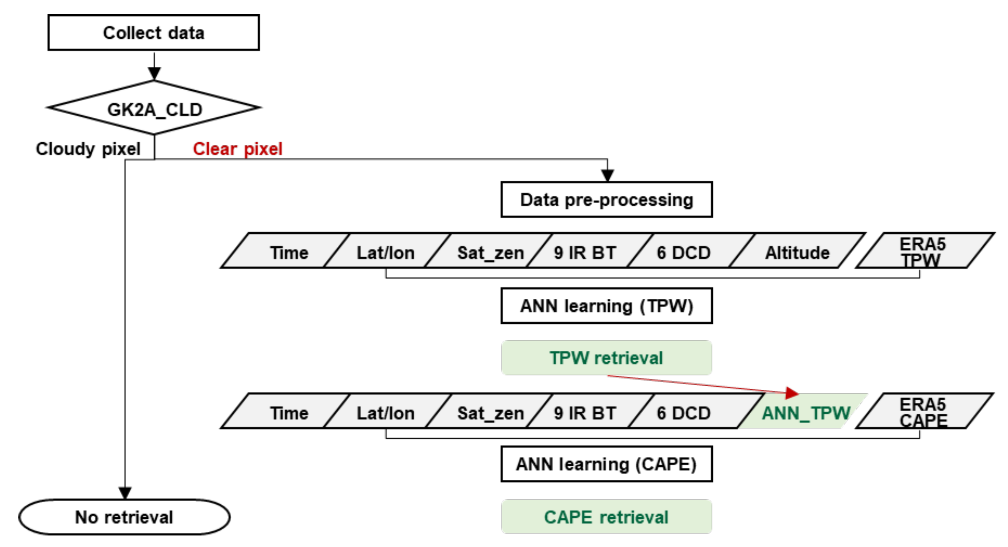
3.1. Retrieval Algorithm Descriptions

The retrieval algorithm of clear-sky TPW and CAPE was developed using IR channels of AMI data. This algorithm was developed based on the machine learning model. We determined to use the ANN model considering the performance and complexity trade-off through a comparison with state-of-the-art models as shown in Appendix A. First of all, as shown in Figure 3, the algorithm starts from the cloud screening using cloud mask products from AMI to extract the clear-sky pixels. In the pre-processing procedure, all input variables from AMI are read and the TPW and CAPE values are calculated from the ERA5 data. For the collocated data, all AMI data are assembled and averaged within the spatial resolution target data. Detailed descriptions of the preparation of the learning dataset are given in Section 3.4. Once all the data are prepared, the neural network model for TPW trains the nonlinear relationship between the input variables and target value through iterative adjustment of the weights in the direction to minimize the errors (see Section 3.2). The retrieved TPW is used in the retrieval algorithm for CAPE as one of the input variables. The neural network model for CAPE is also trained.

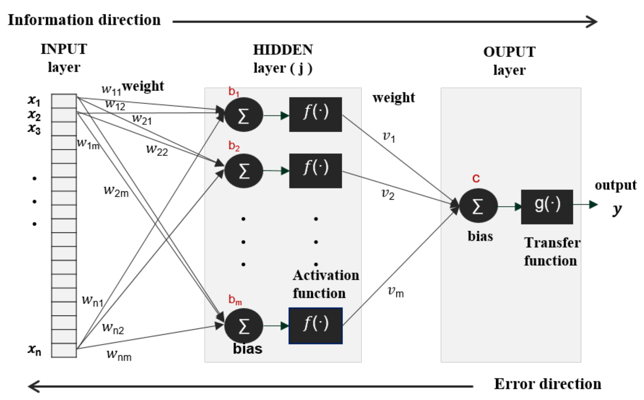
3.2. Conventional ANN Approach (Static Learning)

As one of the most generally used nonlinear machine learning models, ANN based on the multilayer perceptron (MLP) feedforward backpropagation has been successfully applied to the algorithms for estimating meteorological variables using satellite observation data [18,36,37,38]. ANN is inspired by the biological brain composed of networks of neurons to learn higher-order knowledge and solve more complex problems by designing an appropriate architecture [39]. To deal with non-linearity to the network, an activation function transforms the outputs of each layer. In this study, we designed our ANN model with the framework Keras [40] using TensorFlow [41] backend. The ANN hyper-parameters include an activation function, optimizer, and the number of hidden layers, the number of neurons in each hidden layer, the number of iterative training (epoch), and the learning rate.

Through extensive performance tests, the hyper-parameters were empirically determined to work best through a variety of specific set-ups. The architecture of the developed ANN models (Figure 4) consists of the following: one input layer composed of twenty input neurons and one hidden layer composed of forty neurons. The activation function in the hidden layer and output layer is the hyperbolic tangent function and the linear function, respectively. The equation of the final output from the input variables in the ANN model with one hidden layer can be described as:

$$\widehat{y}= \mathrm{g}\left({\displaystyle \sum }_{j=1}^m{\upsilon }_{j}f\left({\displaystyle \sum }_{i=1}^n{w}_{ij}{x}_i+b_j\right)+c\right)$$

(1)

where $\widehat{y}$ is the estimated prediction of the output layer, $x_i$ is the input vector, $w_{ij}$ is the weight between the input node and the hidden node, $v_j$ is the weight between the hidden node and the output node, $b_j$ is the bias in the hidden layer, $c$ is the bias in the output layer, and $f$ and $\mathrm{g}$ are the activation function in the hidden layer and the output layer, respectively.

In the learning process, the objective of the ANN is to minimize the generalization error between the prediction $\widehat{y}$ and the target value $y$. An optimizer is to adjust the model parameters such as weights and bias through an iterative method [42]. For numerically fast and accurate optimization, Adam optimizer [43] is used in this study. The mean squared error is chosen as our loss function for regression problems. The number of iteration and batch sizes are set to 3000 and 256, respectively. Additionally, to reduce unnecessary computation tasks and converge the network quickly, the Min-Max normalization technique scale all input data to values ranging from $-$1 to 1 [44].

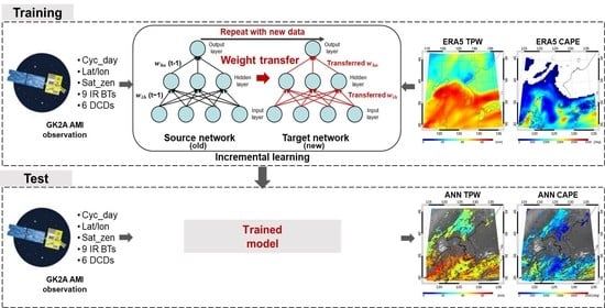
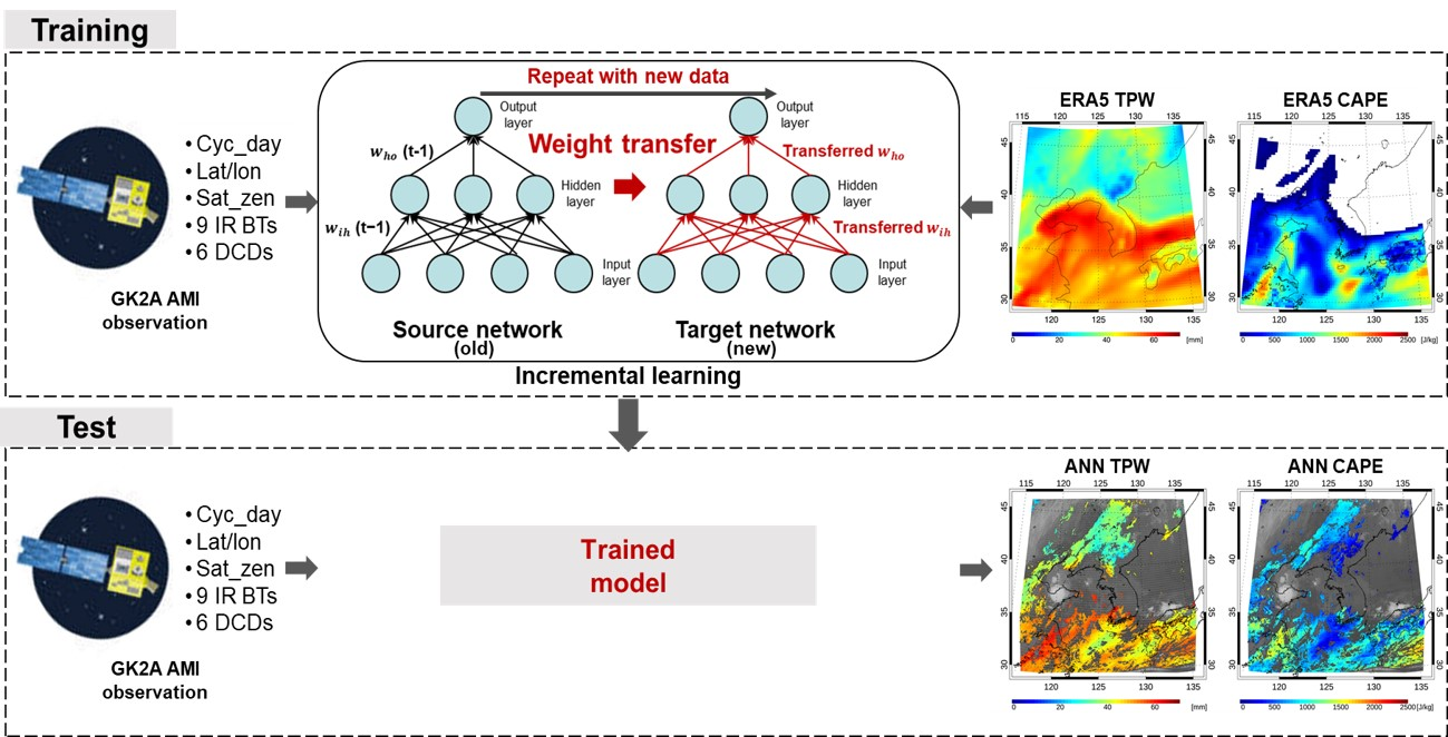
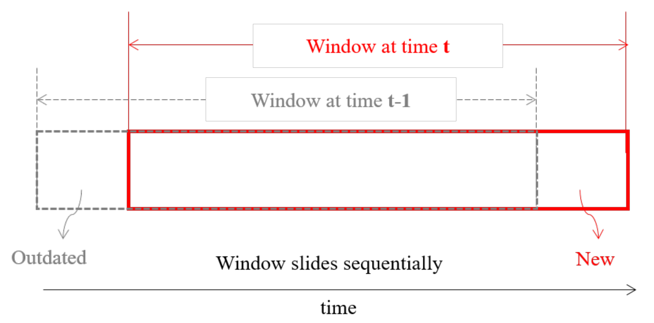
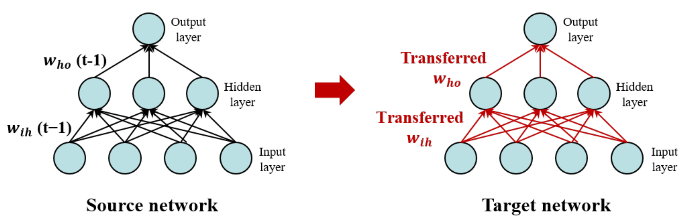
3.3. Incremental Learning Strategies

‘Concept drift’, a term used in the field of machine learning, means that the statistical characteristics of a target variable change over time [45,46]. If the concept drift occurs in the ST ANN, re-training using the entire learning data may not reflect the concept drift. This is because most of the new information is provided by the most recent examples. For the detection of the drift, the error metric is measured and tracked during the test period, where a rise in the error is regarded as an indication of drift [45]. In case of the target concept changing stably or gradually, a new example helps to improve and refine the existing learned model. Adaptation is done by gradually training a new model with current data [47]. In this study, for concept drift adaptation and optimization to preserve the accuracy over time, the ANN model is incrementally and continuously updated based on a sliding window and transferred weights.

In INC learning, a window-based approach that produces compact and representative data, is used [48,49] to handle a huge amount of data constantly coming. This approach incrementally adjusts the previous model using the most recent window. The window represents each block of data which divides the historical data into a period [50]. A sliding window with equal width is utilized in the study to achieve time and space efficiency, although its histogram produces a high variance. Unfortunately, this method may cause any catastrophic forgetting to completely forget any previously learned knowledge [47] when the target concept abruptly changes while the previous window moves to the next window. Therefore, to gradually forget the outdated data and to update the newly arrived data, a sliding temporal window with time steps where the drift does not occur and the error is stable is utilized. The “step size” of the sliding window is the size of the “sliding” action, which is the length of sequence move between each window. Figure 5 shows an example of the process of updating from t − 1 to t.

To find the proper length of the window is challenging. For example, a short length of the sliding window can lead to a big difference and high variance in the next sequence whereas a long one leads to heavy computational load and decreased reactivity of the system [46,51]. To determine an optimal window size in between the two extremes, an empirical experiment that tests error statistics depending on the update cycle from the 1st to the 14th with a one-day interval has been conducted [51,52]. The mean biases of multiple sets corresponding window length during the test period between the retrieved results and target values are calculated and averaged. Figure 6 illustrates mean error values from the test results depending on the different window lengths. As can be seen in Figure 6, for both TPW and CAPE, the mean error decreases as the window length increases up to 10 days. The optimal window length is set to be ten days in consideration of the error statistics (with the nearest value to zero). In addition, considering the similarity between consecutive time steps, the update cycle of this algorithm is set to be one day.

The frequently repeated learning within the sliding window requires high computing resources and tends to fit the local information. To overcome these issues, we propose transfer learning to mitigate these impacts from two aspects. Transfer learning techniques allow models to predict a new task (target network) using learned knowledge from the existing model (source network) [22]. For example, when new samples emerge, the INC learning begins with the transferred weights from a previously learned model as initial weights, to expand the knowledge of the existing model to adapt to new data (Figure 7). Transfer learning techniques should be considered when the source and target domains have similarities.

3.4. Preparation of Learning Dataset

To construct the dataset of the ANN model for the retrieval of TPW and CAPE, GK2A/AMI and ERA5 data were collected in the ELA region.

Table 2. Input variables used to retrieve TPW and CAPE. An abbreviation for each brightness temperature (BT) in channel 8 to 16 is BT8 to BT16, respectively. Dual channel difference is named DCD. The physical property of each input variable is described.

Variable	Physical Property
$\mathrm{BT}8 (6.2 \mathsf{\mu }\mathrm{m}$)	Water vapor in upper tropospheric
$\mathrm{BT}9 (6.9 \mathsf{\mu }\mathrm{m}$)	Water vapor in mid and upper tropospheric
$\mathrm{BT}10 (7.3 \mathsf{\mu }\mathrm{m}$)	Water vapor in mid tropospheric
$\mathrm{BT}11 (8.6 \mathsf{\mu }\mathrm{m}$)	SO2, low level moisture, cloud phase
$\mathrm{BT}12 (9.63 \mathsf{\mu }\mathrm{m}$)	Total ozone, upper air flow
$\mathrm{BT}13 (10.4 \mathsf{\mu }\mathrm{m}$)	Land/sea surface temperature, cloud information, fog, Asian dust, amount of water vapor in lower level, atmospheric motion vector
$\mathrm{BT}14 (11.2 \mathsf{\mu }\mathrm{m}$)
$\mathrm{BT}15 (12.4 \mathsf{\mu }\mathrm{m}$)
$\mathrm{BT}16 (13.3 \mathsf{\mu }\mathrm{m}$)	Air temperature
DCD1 (BT14–BT8)	Moisture in upper tropospheric
DCD2 (BT14–BT9)	Moisture in mid and upper tropospheric
DCD3 (BT14–BT10)	Moisture in mid tropospheric
DCD4 (BT14–BT11)	Amount of water vapor
DCD5 (BT14–BT15)	Split-window channels (amount of water vapor)
DCD6 (BT10–BT8)	Difference between water vapor channels
Cyclic day	Time information
Latitude/Longitude	Geographic information
Satellite zenith angle	Optical depth
Altitude	Topographic information (only use for TPW)
Total precipitable water	Amount of water vapor in the air (only use for CAPE)

describes the input variables of the learning dataset and its physical characteristics. In this study, time and geographic information, satellite zenith angle, and nine IR brightness temperatures (BT) of GK2A/AMI are used as the input variables. The BT at each channel measures different characteristics in the atmosphere. For instance, the atmospheric window channels (BT 11, 13, 14, and 15) indicate the surface properties related to the temperature of land and sea, whereas the water vapor channels (BT8, 9, and 10) show the water vapor in each different mid-level atmosphere. O₃ and CO₂ channels are cooler in the clear sky than the window channels due to the absorption of O₃ and CO₂, respectively [53,54]. In addition, the six dual channel differences (DCD) which represent the amount of water vapor at each level are used. The elevation from DEM data is used only for the retrieval of TPW, and the TPW calculated from ERA5 is used for the retrieval of CAPE.

For the temporal collocation of learning data, AMI data observed at the same time were collected based on the ERA5 data (00, 06, 12, and 18 UTC), and all AMI data are assembled considering the spatial resolution ERA5 data. For example, the clear-sky AMI pixels within 9 $\times$ 9 AMI FOVs centered on the ERA5 grid are selected. Only if more than 100% of the pixels within the 9 $\times$ 9 AMI pixels are clear, they are assembled. Finally, for the collocation and resampling with input and target variables, all collocated clear pixels of AMI data are averaged.

Table 3. Description of period and usage of training and testing dataset.

Method		Period and Usage
Training	Static learning	25 July 2019 to 24 July 2020 (00/06/12/18 UTC)	TPW: 80% (487,135) for training and 20% (121,784) for validation CAPE: 80% (492,478) for training and 20% (123,120) for validation
	Incremental learning	18 July 2020 to 24 July 2021 (00/06/12/18 UTC)	8:2 for training and validation
Testing		25 July 2020 to 24 July 2021 (00/06/12/18 UTC)

describes the period and use of the learning dataset for the ST and INC learning and testing dataset. The ST algorithm requires the training dataset with comprehensive and representative characteristics before the learning [42]. To construct the ST learning dataset, one-year data covering all seasons were selected from the same number of samples every 1 mm for TPW and 50 J/kg for CAPE [55]. Each of about 600,000 independent learning samples are carefully prepared for TPW and CAPE, respectively. The final learning dataset is randomly split into 80% for the training and 20% for the validation. In addition, the test dataset from 25 July 2020 to 24 July 2021 is used. For INC learning, all new clear pixel data every sliding window (ten days) from 18 July 2020 to 24 July 2021 are utilized for learning and all untrained clear pixel data within the update cycle (one day after the period corresponding to the sliding window) 25 July 2020 to 24 July 2021 are used for testing. Like the ST learning, a randomly divided 80% and 20% of INC learning samples were used to learn the ANN model and optimize the hyper-parameters in the ANN model, respectively.

3.5. Accuracy Assessment

For the performances assessment of the proposed retrieval models for TPW and CAPE, three statistical accuracy metrics such as correlation coefficient (R), bias, and root-mean-square-error (RMSE) are used and defined as follows:

$$R=\frac{{{\displaystyle \sum }}_{a=1}^n\left({\widehat{y}}_a-\overline{\widehat{y}}\right)\left(y_a-\overline{y}\right)}{\sqrt{{{\displaystyle \sum }}_{a=1}^n{({\widehat{y}}_a-\overline{\widehat{y}})}^2{{\displaystyle \sum }}_{a=1}^n{(y_a-\overline{y})}^2}}$$

(2)

$$\mathrm{bias}=\frac{1}{n}{\displaystyle \sum }_{a=1}^n({\widehat{y}}_a-y_a)$$

(3)

$$\mathrm{RMSE}=\sqrt{\frac{{{\displaystyle \sum }}_{a=1}^n{({\widehat{y}}_a-y_a)}^2}{n}}$$

(4)

where $y$ is the target value or reference, $\widehat{y}$ is the retrieved value, and n is the number of examples. The Pearson correlation coefficient with values between −1.0 and 1.0 describes the direction and strength of the linear relationship between two variables and is used in this study (Equation (2)). Bias is the averaged deviation between the target and the estimated values between the target value and retrieved value (Equation (3)). RMSE, a formal way to measure the error, is defined as the square root of the average squared error (Equation (4)).

TPW and CAPE estimated from the two different models are compared with the reference data, ERA5 and RAOB, and statistical error metrics are calculated to evaluate the performance based on the collocation criteria. To calculate the statistical validation metrics with ERA5, the clear-sky AMI pixels within 9 $\times$ 9 AMI FOVs centered on the ERA5 grid or RAOB station are selected for the collocation. Only if more than 80% the pixels within the 9 $\times$ 9 AMI pixels are clear, they are averaged and compared. In the case of RAOB, as described in Section 2.3, only quality-controlled data are used. The spatial collocation with RAOB is conducted using all clear-sky GK2A pixels gathered within a 150 km horizontal radius from each RAOB point. The assembled pixels are averaged and compared only when more than 80% of pixels in the domain are clear.

To investigate the characteristics of the models, the accuracy metrics are further analyzed on the temporal and spatial domains. The error statistics (bias and RMSE) over time are monitored and compared for about one year of the test period to check the model stability over time and to examine the seasonal variability. The collocated data are averaged over a week to reduce frequent fluctuations and to clearly show the trends. Additionally, autocorrelation (AC) is utilized to quantify and compare the temporal variability as shown in the following equation:

$$\mathrm{AC}=\frac{{{\displaystyle \sum }}_{t=0}^{N-L-1}\left(x_t-\overline{x}\right)\left(x_{t+L}-\overline{x}\right)}{{{\displaystyle \sum }}_{t=0}^{N-1}{\left(x_t-\overline{x}\right)}^2}$$

(5)

where $N$ is the number of data, $\mathrm{t}$ is the index of the date, $L$ is time lag, $x$ and $\overline{x}$ is the bias and globally averaged bias, respectively. Mathematically, AC means the degree of similarity between observations as a function of the time lag between the time series data. The AC values can be analyzed to measure how much past values influence the current values with values ranging from −1.0 and 1.0. The spatial distribution of errors in the ST and INC ANN models are compared using ERA5 data in the ELA region during the testing period.

Additionally, to clarify the relative contribution of input variables to the final estimation, permutation feature importance is used [56]. This is a method to determine the variable importance through how much a feature affects performance loss when it is not used. In order not to use the specific feature, instead of excluding the variable, the feature is randomly mixed (permutation) and the feature is recognized as noise. Since it is applied in the test stage after learning, it has the advantage of not requiring re-training. The values of the difference between test results using the data that the certain feature is permuted and the original test result is calculated and compared.

4. Results

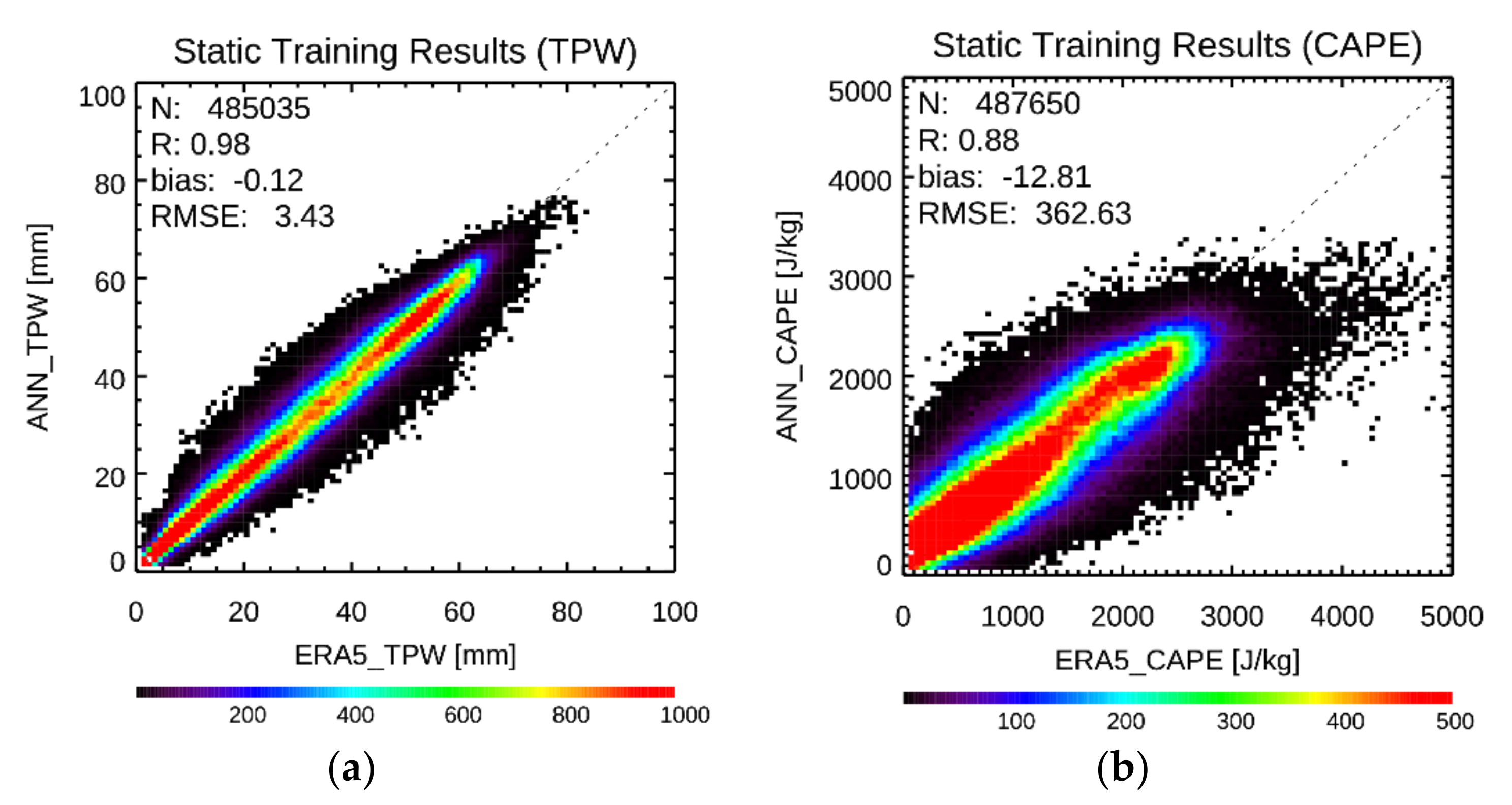
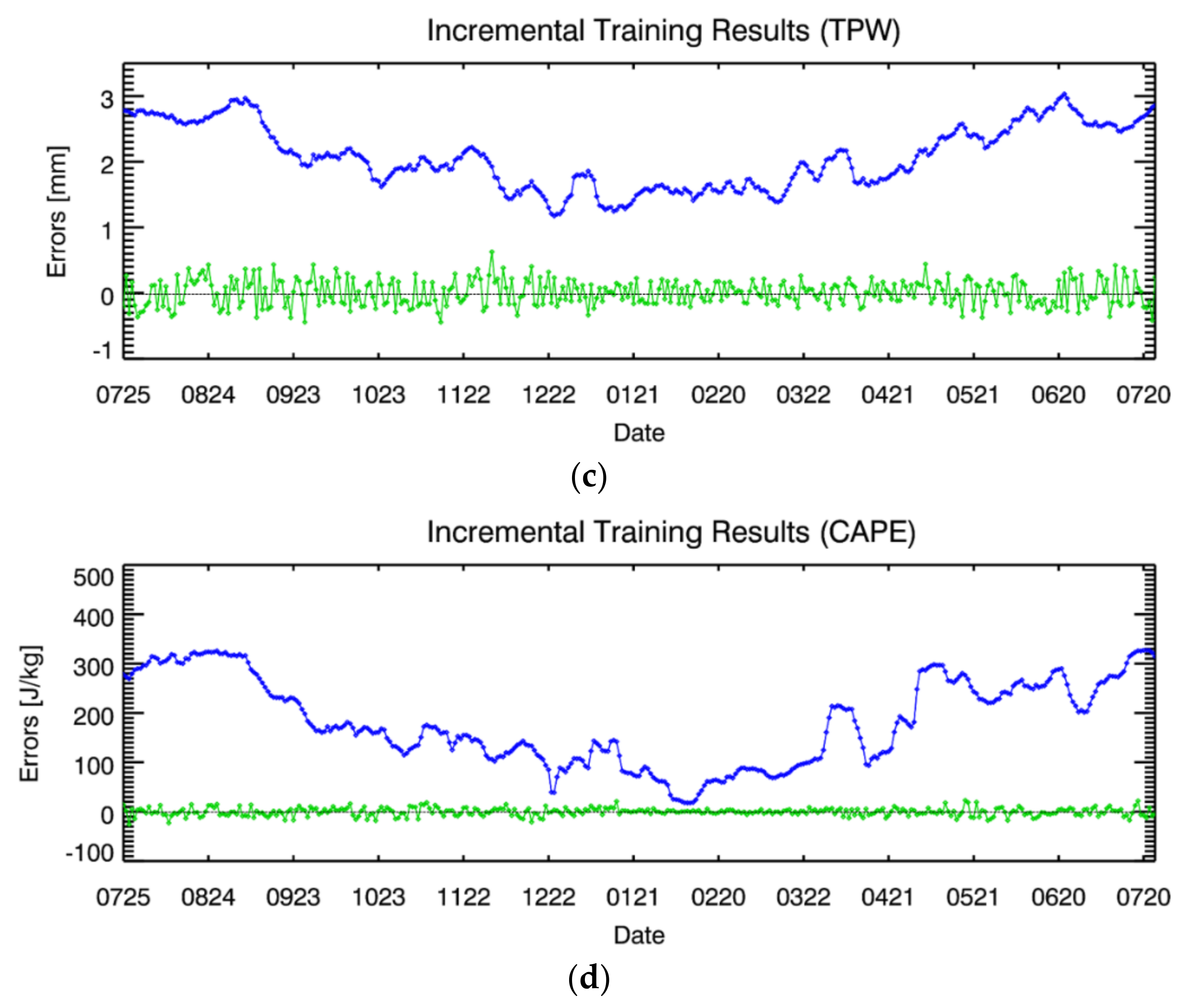
4.1. Model Performance

Figure 8 depicts the training performance of the ST and INC learning models for TPW and CAPE during the periods from 25 July 2019 to 24 July 2020 for the ST learning and from 25 July 2020 to 24 July 2021 for INC learning. The bias, RMSE, and R of the ST ANN are –0.12 mm, 3.43 mm, and 0.98 for TPW and −12.81 J/kg, 362.63 J/kg, and 0.88 for CAPE, respectively (Figure 8a,b). The training results of the INC ANN model are shown as time series graphs since the INC learning is continuously trained over time in Figure 8c,d. INC algorithm has the biases fluctuating with a small width based on the zero value for both variables and RMSE ranging from 1 mm to 3 mm and 0 J/kg to 300 J/kg in TPW and CAPE, respectively. According to the training results, it is clear that the INC algorithm for TPW and CAPE outperforms the ST ANN model in terms of model performance.

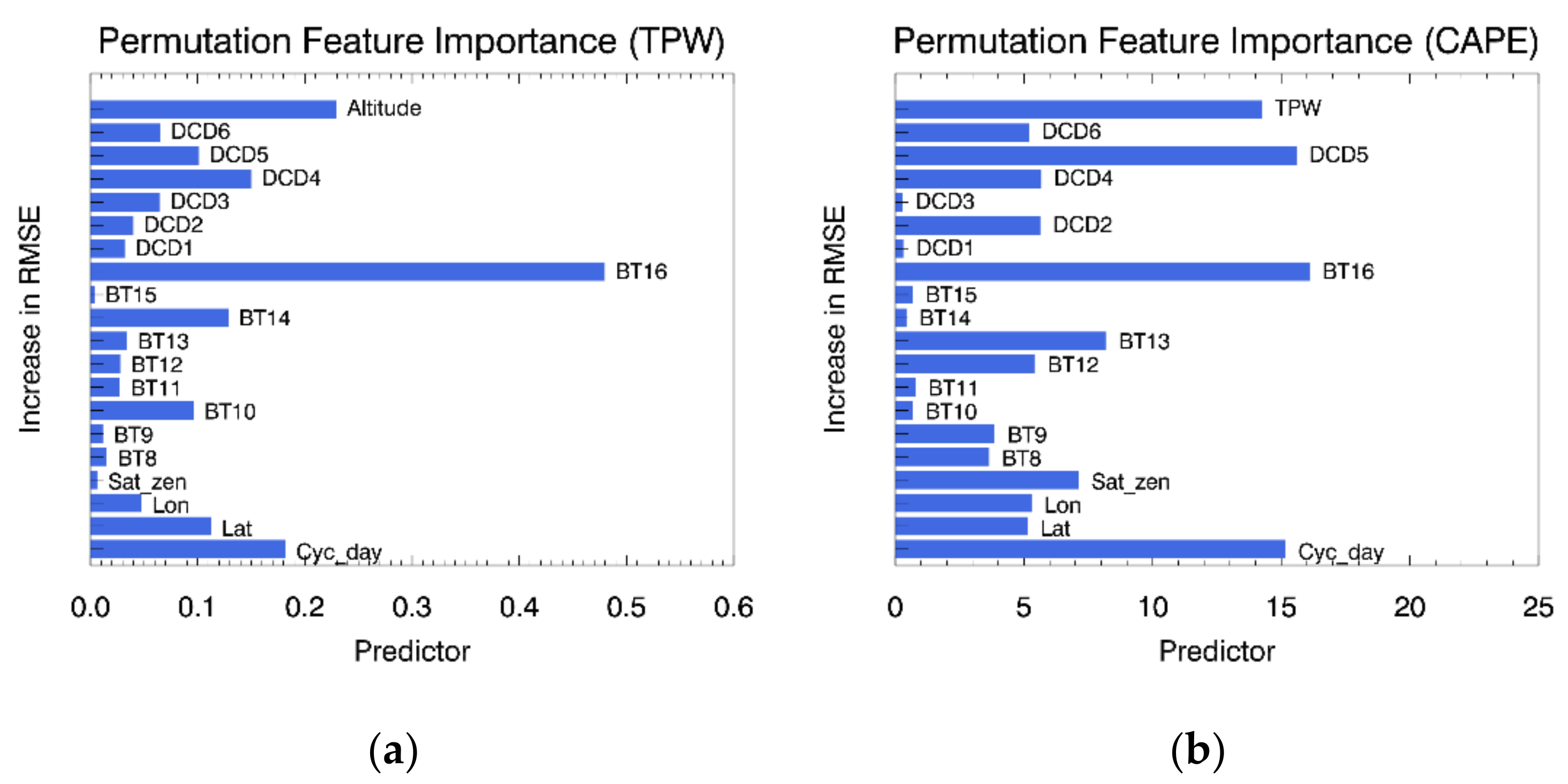
4.2. Feature Contributions

To identify how much each input variable contributes to the ANN model, the calculated differences of RMSE by permutation feature importance are compared. In Figure 9, the length of the bar indicates the RMSE difference. In both TPW and CAPE, BT16 is diagnosed as a main contributing variable. The BT16, the carbon dioxide absorption channel, apparently shows the surface features in clear air [54]. DCD4, DCD5, and cyc_day are considered the next significant input variables having a strong contribution to the estimation of both TPW and CAPE. The window channel differences—DCD4 and DCD5—represent the amount of water vapor. Cyc_day means the date which impacts temperature and humidity in the atmosphere. Altitude and TPW are also identified as explanatory predictors for the TPW and CAPE, respectively. As analyzed in [18], altitude is one of the important input variables for the estimation of TPW, which is the sum of water vapor in the air column. In addition, variables related to water vapor amounts such as the difference between the clean window channel and water vapor channel (e.g., DCD1, DCD2, and DCD3) exhibit relatively high magnitudes. Thus, it is clear that the window channel giving clear information of the surface temperature and DCDs representing the amount of moisture in each layer of the atmosphere have high variable importance.

4.3. Evaluation Results and Comparison

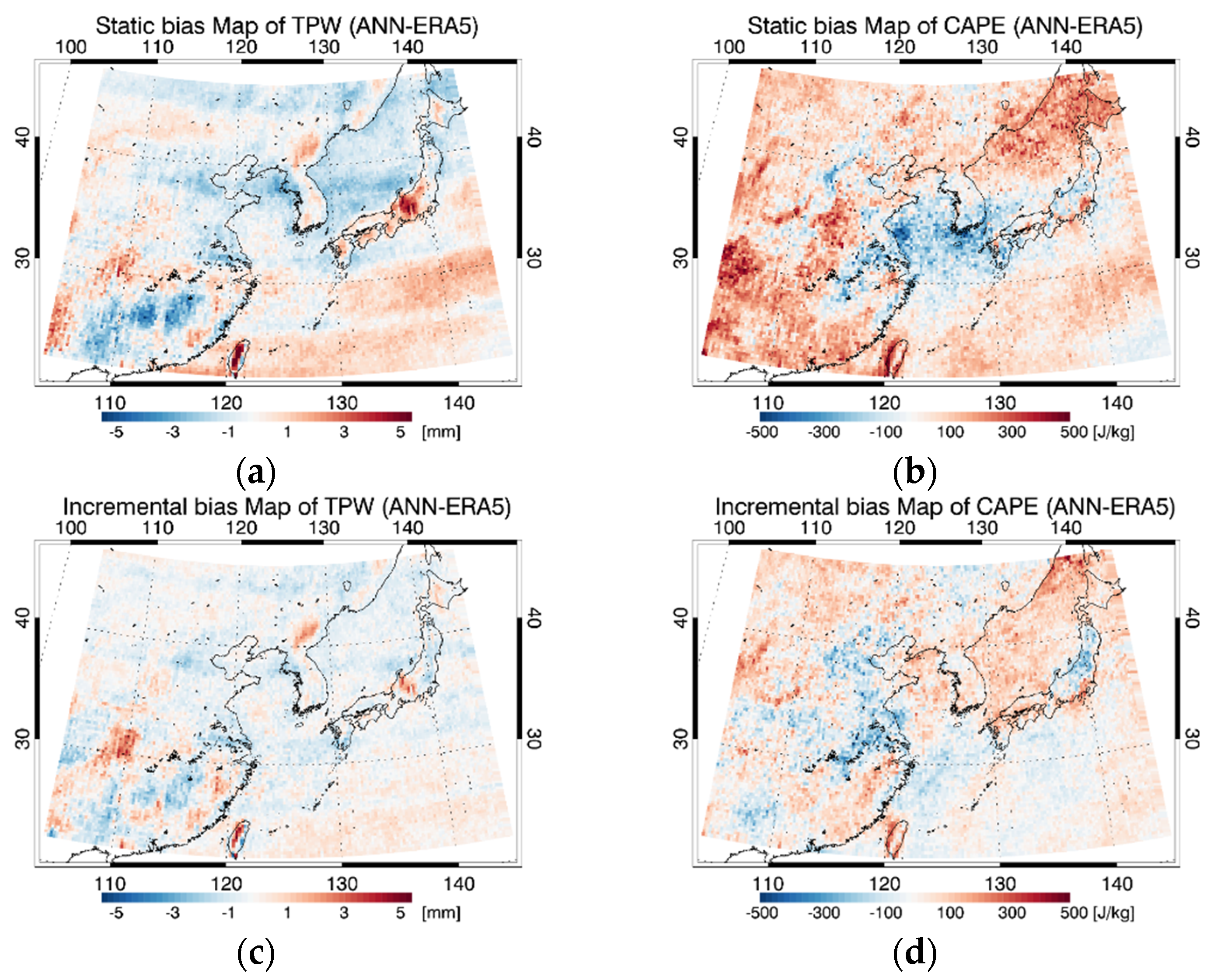
To quantitatively validate each learning model and compare results from the models, the observed AMI data from the period not used in the learning process were utilized.

Table 4. Accuracy assessment based on ERA5 and RAOB for the ST and INC NN model in the ELA region during the test period. Evaluation metrics (i.e., bias, RMSE, and R) are calculated.

	Static NN			Incremental NN
	Bias	RMSE	R	Bias	RMSE	R
ERA5_TPW	0.11	3.43	0.97	0.04	3.17	0.98
ERA5_CAPE	3.65	516.62	0.74	−9.69	461.50	0.80
RAOB_TPW	0.23	5.05	0.95	−0.17	4.39	0.96
RAOB_CAPE	338.10	700.81	0.56	251.70	619.28	0.65

summarizes the overall error statistics (averaged bias, RMSE, and R) between the target values and estimated values from models at the ELA region during the testing period. For the comparison with ERA5, about five and one million collocated data are used for TPW and CAPE, respectively. The ST and INC algorithm gives 0.11 and 0.04 mm of bias and 3.43 and 3.17 mm of RMSE for TPW, and 3.65 and −9.69 J/kg of bias, 516.62 and 461.50 J/kg of RMSE for CAPE, respectively.

Untrained datasets from RAOB were also utilized to verify the accuracy of the developed algorithms. As described in Section 2.3, only quality-controlled data were used, which remains are a relatively small number of collocated data (one million for TPW and one thousand for CAPE collocation data over the clear-sky conditions) compared with the number of ERA5. As shown in Table 4, in the comparison with RAOB, the INC model gives improved error statistics compared to the ST learning, having 26% decreased bias for TPW and 26% for CAPE. RMSE is also reduced by about 13% and 12% in TPW and CAPE with the INC model. These test results demonstrate that the INC algorithm outperforms when compared to the ST ANN model.

4.4. Error Analysis

In addition to the evaluation of accuracy, the model stability and the error statistics (bias and RMSE) over time are monitored for about one year of the test period. The bias displayed large variability in the ST algorithm, whereas INC learning has a bias closer to zero for both TPW and CAPE. As shown in Figure 10, RMSE shows almost similar values in both models but showed slightly lower values in the INC model compared to the ST model. RMSE also tended to be high in hot and humid summer and low in cold and dry winter regardless of the variables.

Table 5. Autocorrelation values of the bias for the static and incremental ANN model in ELA region during test period. The time lag is set to one day.

	Static ANN	Incremental ANN
TPW	0.76	0.52
CAPE	0.79	0.32

reveals the AC values of the biases calculated by setting the time lag to one day. AC values from the INC algorithm are lower than those from the ST ANN model for both TPW and CAPE, which implies that the test results from the INC model are less temporally related and stationary over time. According to the results, it is clear that the gradual learning results, which are immediately reflected in the latest training data, are more stable and less sensitive to time error statistics compared to the conventional ST learning results.

Figure 11 displays the spatial distribution map of the test errors for TPW and CAPE of ST and INC learning, compared to ERA5 in the ELA region during the testing period. First of all, the INC ANN model (Figure 11c,d) reveals a remarkably lower bias when compared to the ST ANN model for both TPW and CAPE. The ST ANN model reveals relatively high bias values overall.

Meanwhile, in the case of the TPW bias map, a striping with blue-shaded negative bias was identified in both ANN models as shown in Figure 11a,c. In the case of CAPE, the striping features are not prominently observed. The striping issue is due to the calibration problems in GK2A/AMI CO₂ channel [57] and the striping feature also appears in the retrieved results of the developed models which utilize the original high-resolution GK2A data. Additionally, the tendency to overestimate TPW over the regions that have relatively lower surface pressure (relatively higher terrain elevation) is reduced compared to the previous result [18] by adding altitude as an input variable in the INC model result, but it is still prominent in the ST model result.

5. Discussion

This is the first study conducted to estimate TPW and CAPE at the same time from GK2A/AMI data in Northeast Asia using the INC ANN model. This study proposed a novel method that continuously learns and immediately reflects new trend data by using the sliding window and adjusting the transferred weights from previous learning. The evaluation results demonstrate that the INC algorithm significantly improves the accuracy for TPW and CAPE compared with the conventional approach (the ST learning). The error statistics from the INC learning results are analyzed to have lower spatiotemporal variability. It should also be noted that the INC algorithm is applicable without a sufficient training set that contains all necessary knowledge before learning. With this advantage, it can be utilized where the training sets which are representative and comprehensive are too big, the target concepts change over time, and the learning samples can be assembled over time such as time-series data. Therefore, it might be feasible in real-time operations considering time, storage, or other costs.

When used with the rapid scan data with high spatial (2 km) and temporal (2 min for the full-scan) resolution, the INC ANN-derived instability and moisture would provide useful information prior to the outbreak of a severe convective storm. Furthermore, these high-resolution products can provide promising information even among the cloudy images despite the clear-sky output for severe convective weather forecasting through near-real-time monitoring. To evaluate the possible application of the proposed algorithm for a localized short-term prediction of severe weather caused by intense convective weather systems, we plan to develop a pixel-based machine learning model to detect severe convective rainfall using atmospheric parameters from the developed model. GK2A data with high spatiotemporal resolution will be used for the early warning of intense convective systems that develop and disappear rapidly. To define the severe weather associated with heavy rainfall, radar reflectivity with more than 35 dBZ values which identify the threshold of the occurrence of the convective severe weather [58] during a long-term period will be utilized. Finally, the retrieved clear TPW and CAPE from the developed model using GK2A data and the radar reflectivity value are used as predictors and a predictive and target value of the detection algorithm-based machine learning model, respectively.

In this study, the INC ANN model is developed with the fixed model complexity determined from learning using the first data. When new samples emerge, each learned weight is transferred from the previous network to the next network which has an identical model structure. However, since the model complexity can grow and shrink to optimally integrate new knowledge, there is a possibility for improvement of the model performance. Another important consideration regarding the architecture of INC learning is the appropriate setting of the sliding window approach. In this study, the length of the window and update cycle are empirically examined. Future work can consider a more objective methodology for optimal settings to improve accuracy. For example, the current INC algorithm has not yet fully considered all possible cases including data absence or quality abnormality of input/output data, which can cause sudden model performance degradation and thus needs to be considered. Although for a short time, the transferred previous weights can be used, in the long term, the improvement of the algorithm should be considered to maintain the stability of the model.

6. Conclusions

In this study, the retrieval algorithm of TPW and CAPE based on the ANN model was developed using AMI, a pseudo-sounding imager onboard the geostationary GK2A satellite, over Northeast Asia to monitor the pre-convective environments. The implementation of INC learning in the ANN model can adapt to changes in the target property before having a comprehensive and sufficient learning dataset. To extend the existing model’s knowledge by gradually forgetting the outdated data when new data arrives to update, the INC approach using the transfer learning based on a sliding window with ten days for the window length and one day for time step is presented. Time and geographic information, satellite zenith angle, nine AMI IR BTs (covering 6.2 to 13.3 $\mathsf{\mu }\mathrm{m}$ wavelength range), six dual channel differences, altitude (only for TPW retrieval), and TPW (only for CAPE retrieval) were used as the input variables whereas the corresponding TPW and CAPE calculated from the atmospheric sounding of ERA5 data were used as an output value. Each hyper-parameter of the ANN model was optimized using the validation datasets (20% of whole learning). BT16 and DCDs between the window channels, which measure temperature and amount of moisture near the surface, are diagnosed as mainly contributing variables to the retrieval of TPW and CAPE in the ANN model. The RAOB data are used for the model evaluation and comparison with the ST ANN model. When compared to RAOB, the INC ANN model shows better performance in evaluation metrics (the accuracy of TPW and CAPE decreased by approximately 26% and 26% for bias and about 13% and 12% for RMSE, respectively). According to the error analysis, it is clear that the INC algorithm produces temporally more stable and spatially lower errors than the ST algorithm. Considering the much finer spatiotemporal resolution of AMI on the GK2A (every 2 min with a spatial resolution of approximately 2 km), the estimated TPW and CAPE are anticipated to provide quite helpful information for near-real-time monitoring to diagnose the genesis, evolution, and fine structure of rapid evolving meteorological events. In addition, the weather forecasting application of the retrieved TPW and CAPE together with wind components will be conducted in pre-convective atmospheric conditions.

References

1. Koutavarapu, R.; Umakanth, N.; Satyanarayana, T.; Kumar, M.S.; Rao, M.C.; Lee, D.-Y.; Shim, J. Study of Statistical Estimated Parameters Using ERA5 Reanalysis Data over Khulna Region during Monsoon Season. Acta Geophys. 2021, 69, 1963–1978. [Google Scholar] [CrossRef]
2. Botes, D.; Mecikalski, J.R.; Jedlovec, G.J. Atmospheric Infrared Sounder (AIRS) Sounding Evaluation and Analysis of the Pre-Convective Environment: Pre-Convective Airs Sounding Analysis. J. Geophys. Res. 2012, 117, 1–22. [Google Scholar] [CrossRef]
3. Kwon, T.-Y.; Kim, J.-S.; Kim, B.-G. Comparison of the Properties of Yeongdong and Yeongseo Heavy Rain. Atmosphere 2013, 23, 245–264. [Google Scholar] [CrossRef] [Green Version]
4. Kim, Y.-C.; Ham, S.-J. Heavy Rainfall prediction using convective instability index. J. Korean Soc. Aviat. Aeronaut. 2009, 17, 17–23. [Google Scholar]
5. Jung, S.-P.; Kwon, T.-Y.; Han, S.-O.; Jeong, J.-H.; Shim, J.; Choi, B.-C. Thermodynamic Characteristics Associated with Localized Torrential Rainfall Events in the Southwest Region of the Korean Peninsula. Asia-Pac. J. Atmos. Sci. 2015, 51, 229–237. [Google Scholar] [CrossRef]
6. McNulty, R.P. Severe and Convective Weather: A Central Region Forecasting Challenge. Weather Forecast. 1995, 10, 187–202. [Google Scholar] [CrossRef]
7. Kulikov, M.Y.; Belikovich, M.V.; Skalyga, N.K.; Shatalina, M.V.; Dementyeva, S.O.; Ryskin, V.G.; Shvetsov, A.A.; Krasil’nikov, A.A.; Serov, E.A.; Feigin, A.M. Skills of Thunderstorm Prediction by Convective Indices over a Metropolitan Area: Comparison of Microwave and Radiosonde Data. Remote Sens. 2020, 12, 604. [Google Scholar] [CrossRef] [Green Version]
8. Gartzke, J.; Knuteson, R.; Przybyl, G.; Ackerman, S.; Revercomb, H. Comparison of Satellite-, Model-, and Radiosonde-Derived Convective Available Potential Energy in the Southern Great Plains Region. J. Appl. Meteor. Climatol. 2017, 56, 1499–1513. [Google Scholar] [CrossRef]
9. Bevis, M.; Businger, S.; Herring, T.A.; Rocken, C.; Anthes, R.A.; Ware, R.H. GPS Meteorology: Remote Sensing of Atmospheric Water Vapor Using the Global Positioning System. J. Geophys. Res. Atmos. 1992, 97, 15787–15801. [Google Scholar] [CrossRef]
10. Liu, Z.; Min, M.; Li, J.; Sun, F.; Di, D.; Ai, Y.; Li, Z.; Qin, D.; Li, G.; Lin, Y.; et al. Local Severe Storm Tracking and Warning in Pre-Convection Stage from the New Generation Geostationary Weather Satellite Measurements. Remote Sens. 2019, 11, 383. [Google Scholar] [CrossRef] [Green Version]
11. Lee, J.; Lee, S.-W.; Han, S.-O.; Lee, S.-J.; Jang, D.-E. The Impact of Satellite Observations on the UM-4DVar Analysis and Prediction System at KMA. Atmosphere 2011, 21, 85–93. [Google Scholar] [CrossRef]
12. Mecikalski, J.R.; Rosenfeld, D.; Manzato, A. Evaluation of Geostationary Satellite Observations and the Development of a 1–2 h Prediction Model for Future Storm Intensity. J. Geophys. Res. Atmos. 2016, 121, 6374–6392. [Google Scholar] [CrossRef]
13. Kim, D.; Gu, M.; Oh, T.-H.; Kim, E.-K.; Yang, H.-J. Introduction of the Advanced Meteorological Imager of Geo-Kompsat-2a: In-Orbit Tests and Performance Validation. Remote Sens. 2021, 13, 1303. [Google Scholar] [CrossRef]
14. Li, Z.; Li, J.; Menzel, W.P.; Schmit, T.J.; Nelson, J.P.; Daniels, J.; Ackerman, S.A. GOES Sounding Improvement and Applications to Severe Storm Nowcasting. Geophys. Res. Lett. 2008, 35. [Google Scholar] [CrossRef] [Green Version]
15. Jin, X.; Li, J.; Schmit, T.J.; Li, J.; Goldberg, M.D.; Gurka, J.J. Retrieving Clear-Sky Atmospheric Parameters from SEVIRI and ABI Infrared Radiances. J. Geophys. Res. Atmos. 2008, 113. [Google Scholar] [CrossRef]
16. Lee, S.J.; Ahn, M.-H.; Chung, S.-R. Atmospheric Profile Retrieval Algorithm for Next Generation Geostationary Satellite of Korea and Its Application to the Advanced Himawari Imager. Remote Sens. 2017, 9, 1294. [Google Scholar] [CrossRef] [Green Version]
17. Basili, P.; Bonafoni, S.; Mattioli, V.; Pelliccia, F.; Ciotti, P.; Carlesimo, G.; Pierdicca, N.; Venuti, G.; Mazzoni, A. Neural-Network Retrieval of Integrated Precipitable Water Vapor over Land from Satellite Microwave Radiometer. In Proceedings of the 2010 11th Specialist Meeting on Microwave Radiometry and Remote Sensing of the Environment, Washington, DC, USA, 1–4 March 2010; pp. 161–166. [Google Scholar]
18. Lee, Y.; Han, D.; Ahn, M.-H.; Im, J.; Lee, S.J. Retrieval of Total Precipitable Water from Himawari-8 AHI Data: A Comparison of Random Forest, Extreme Gradient Boosting, and Deep Neural Network. Remote Sens. 2019, 11, 1741. [Google Scholar] [CrossRef] [Green Version]
19. Mallet, C.; Moreau, E.; Casagrande, L.; Klapisz, C. Determination of Integrated Cloud Liquid Water Path and Total Precipitable Water from SSM/I Data Using a Neural Network Algorithm. Int. J. Remote Sens. 2002, 23, 661–674. [Google Scholar] [CrossRef]
20. Hecht-Nielsen, R. III.3—Theory of the Backpropagation Neural Network**Based on “Nonindent”. In Neural Networks for Perception, Proceedings of the International Joint Conference on Neural Networks, Washington, DC, USA, 18–22 June 1989; Wechsler, H., Ed.; Academic Press: Cambridge, MA, USA, 1992; pp. 65–93. ISBN 978-0-12-741252-8. [Google Scholar]
21. Gamage, S.; Premaratne, U. Detecting and Adapting to Concept Drift in Continually Evolving Stochastic Processes. In Proceedings of the International Conference on Big Data and Internet of Thing, London, UK, 20–22 December 2017; Association for Computing Machinery: New York, NY, USA, 2017; pp. 109–114. [Google Scholar]
22. Andrade, M.; Gasca, E.; Rendón, E. Implementation of Incremental Learning in Artificial Neural Networks. In Proceedings of the 3rd Global Con- ference on Artificial Intelligence, Miami, FL, USA, 18–22 October 2017; EasyChair: Manchester, UK, 2017; Volume 50, pp. 221–232. [Google Scholar]
23. Tasar, O.; Tarabalka, Y.; Alliez, P. Incremental Learning for Semantic Segmentation of Large-Scale Remote Sensing Data. IEEE J. Sel. Top. Appl. Earth Obs. Remote Sens. 2019, 12, 3524–3537. [Google Scholar] [CrossRef] [Green Version]
24. Xiao, T.; Zhang, J.; Yang, K.; Peng, Y.; Zhang, Z. In Proceedings of the 22nd ACM International Conference on Multimedia Virtual Event, Online, 3–7 November 2014; Association for Computing Machinery: New York, NY, USA, 2014; pp. 177–186.
25. Bruzzone, L.; Fernàndez Prieto, D. An Incremental-Learning Neural Network for the Classification of Remote-Sensing Images. Pattern Recognit. Lett. 1999, 20, 1241–1248. [Google Scholar] [CrossRef]
26. Li, X.; Du, Z.; Huang, Y.; Tan, Z. A Deep Translation (GAN) Based Change Detection Network for Optical and SAR Remote Sensing Images. ISPRS J. Photogramm. Remote Sens. 2021, 179, 14–34. [Google Scholar] [CrossRef]
27. Zhan, Y.; Qin, J.; Huang, T.; Wu, K.; Hu, D.; Zhao, Z.; Wang, Y.; Cao, Y.; Jiao, R.; Medjadba, Y.; et al. Hyperspectral Image Classification Based on Generative Adversarial Networks with Feature Fusing and Dynamic Neighborhood Voting Mechanism. In Proceedings of the IGARSS 2019—2019 IEEE International Geoscience and Remote Sensing Symposium, Yokohama, Japan, 28 July–2 August 2019; pp. 811–814. [Google Scholar]
28. Tuller, S.E. World Distribution of Mean Monthly and Annual Precipitable Water. Mon. Weather Rev. 1968, 96, 785–797. [Google Scholar] [CrossRef]
29. Durre, I.; Vose, R.S.; Wuertz, D.B. Overview of the Integrated Global Radiosonde Archive. J. Clim. 2006, 19, 53–68. [Google Scholar] [CrossRef] [Green Version]
30. Dai, A.; Wang, J.; Thorne, P.W.; Parker, D.E.; Haimberger, L.; Wang, X.L. A New Approach to Homogenize Daily Radiosonde Humidity Data. J. Clim. 2011, 24, 965–991. [Google Scholar] [CrossRef]
31. Zhang, W.; Lou, Y.; Haase, J.S.; Zhang, R.; Zheng, G.; Huang, J.; Shi, C.; Liu, J. The Use of Ground-Based GPS Precipitable Water Measurements over China to Assess Radiosonde and ERA-Interim Moisture Trends and Errors from 1999 to 2015. J. Clim. 2017, 30, 7643–7667. [Google Scholar] [CrossRef]
32. Persson, A. User Guide to ECMWF Forecast Products. 2001; p. 107. Available online: https://ghrc.nsstc.nasa.gov/uso/ds_docs/tcsp/tcspecmwf/ECMWFUserGuideofForecastProductsm32.pdf (accessed on 5 December 2021).
33. Hersbach, H.; Bell, B.; Berrisford, P.; Hirahara, S.; Horányi, A.; Muñoz-Sabater, J.; Nicolas, J.; Peubey, C.; Radu, R.; Schepers, D.; et al. The ERA5 Global Reanalysis. Q. J. R. Meteorol. Soc. 2020, 146, 1999–2049. [Google Scholar] [CrossRef]
34. Hensley, S.; Rosen, P.; Gurrola, E. The SRTM Topographic Mapping Processor. In Proceedings of the IGARSS 2000. IEEE 2000 International Geoscience and Remote Sensing Symposium. Taking the Pulse of the Planet: The Role of Remote Sensing in Managing the Environment. Proceedings (Cat. No.00CH37120), Honolulu, HI, USA, 24–28 July 2000; IEEE: Honolulu, HI, USA, July 2000; Volume 3, pp. 1168–1170. [Google Scholar]
35. Berry, P.A.M.; Garlick, J.D.; Smith, R.G. Near-Global Validation of the SRTM DEM Using Satellite Radar Altimetry. Remote Sens. Environ. 2007, 106, 17–27. [Google Scholar] [CrossRef]
36. Blackwell, W.J. A Neural-Network Technique for the Retrieval of Atmospheric Temperature and Moisture Profiles from High Spectral Resolution Sounding Data. IEEE Trans. Geosci. Remote Sens. 2005, 43, 2535–2546. [Google Scholar] [CrossRef]
37. Koenig, M.; de Coning, E. The MSG Global Instability Indices Product and Its Use as a Nowcasting Tool. Weather Forecast. 2009, 24, 272–285. [Google Scholar] [CrossRef]
38. Martinez, M.A.; Velazquez, M.; Manso, M.; Mas, I. Application of LPW and SAI SAFNWC/MSG Satellite Products in Pre-Convective Environments. Atmos. Res. 2007, 83, 366–379. [Google Scholar] [CrossRef]
39. Atkinson, P.M.; Tatnall, A.R.L. Introduction Neural Networks in Remote Sensing. Int. J. Remote Sens. 1997, 18, 699–709. [Google Scholar] [CrossRef]
40. Chollet, F. Deep Learning with Python; Simon and Schuster: New York, NY, USA, 2017; ISBN 978-1-63835-204-4. [Google Scholar]
41. Abadi, M.; Barham, P.; Chen, J.; Chen, Z.; Davis, A.; Dean, J.; Devin, M.; Ghemawat, S.; Irving, G.; Isard, M.; et al. TensorFlow: A System for Large-Scale Machine Learning; UNSENIX: Berkeley, CA, USA, 2016; pp. 265–283. [Google Scholar]
42. Blackwell, W.J.; Chen, F.W. Neural Networks in Atmospheric Remote Sensing; Artech House: Norwood, MA, USA, 2009; ISBN 978-1-59693-373-6. [Google Scholar]
43. Kingma, D.P.; Ba, J. Adam: A Method for Stochastic Optimization. arXiv 2017, arXiv:1412.6980. [Google Scholar]
44. Jin, J.; Li, M.; Jin, L. Data Normalization to Accelerate Training for Linear Neural Net to Predict Tropical Cyclone Tracks. Math. Probl. Eng. 2015, 2015, e931629. [Google Scholar] [CrossRef] [Green Version]
45. Casillas, J.; Wang, S.; Yao, X. Concept Drift Detection in Histogram-Based Straightforward Data Stream Prediction. In Proceedings of the 2018 IEEE International Conference on Data Mining Workshops (ICDMW), Singapore, 17–20 November 2018; pp. 878–885. [Google Scholar]
46. Gepperth, A.; Hammer, B. Incremental Learning Algorithms and Applications. In Proceedings of the European Symposium on Artificial Neural Networks (ESANN), Bruges, Belgium, 27–29 April 2016. [Google Scholar]
47. Gama, J.; Medas, P.; Castillo, G.; Rodrigues, P. Learning with Drift Detection. In Advances in Artificial Intelligence—SBIA 2004, Proceedings of the 17th Brazilian Symposium on Artificial Intelligence, Sao Luis, Brazil, 29 September–1 Ocotber 2004; Bazzan, A.L.C., Labidi, S., Eds.; Springer: Berlin/Heidelberg, Germany, 2004; pp. 286–295. [Google Scholar]
48. Guha, S.; Koudas, N.; Shim, K. Approximation and Streaming Algorithms for Histogram Construction Problems. ACM Trans. Database Syst. 2006, 31, 396–438. [Google Scholar] [CrossRef]
49. Sebastião, R.; Gama, J.; Mendonça, T. Constructing Fading Histograms from Data Streams. Prog. Artif. Intell. 2014, 3, 15–28. [Google Scholar] [CrossRef] [Green Version]
50. Wang, H.; Fan, W.; Yu, P.S.; Han, J. Mining Concept-Drifting Data Streams Using Ensemble Classifiers. In Proceedings of the Ninth ACM SIGKDD International Conference on Knowledge Discovery and Data Mining, Washington, DC, USA, 24 August 2003; Association for Computing Machinery: New York, NY, USA, 2003; pp. 226–235. [Google Scholar]
51. Oskoei, M.A.; Hu, H. Support Vector Machine-Based Classification Scheme for Myoelectric Control Applied to Upper Limb. IEEE Trans. Biomed. Eng. 2008, 55, 1956–1965. [Google Scholar] [CrossRef]
52. Smith, L.H.; Hargrove, L.J.; Lock, B.A.; Kuiken, T.A. Determining the Optimal Window Length for Pattern Recognition-Based Myoelectric Control: Balancing the Competing Effects of Classification Error and Controller Delay. IEEE Trans. Neural Syst. Rehabil. Eng. 2011, 19, 186–192. [Google Scholar] [CrossRef] [Green Version]
53. Ebell, K.; Orlandi, E.; Hünerbein, A.; Löhnert, U.; Crewell, S. Combining Ground-Based with Satellite-Based Measurements in the Atmospheric State Retrieval: Assessment of the Information Content. J. Geophys. Res. Atmos. 2013, 118, 6940–6956. [Google Scholar] [CrossRef]
54. Schmit, T.J.; Lindstrom, S.S.; Gerth, J.J.; Gunshor, M.M. Applications of the 16 Spectral Bands on the Advanced Baseline Imager (ABI). 2018. Available online: http://nwafiles.nwas.org/jom/articles/2018/2018-JOM4/2018-JOM4.pdf (accessed on 5 December 2021).
55. Yu, L.; Wang, S.; Lai, K.K. An Integrated Data Preparation Scheme for Neural Network Data Analysis. IEEE Trans. Knowl. Data Eng. 2006, 18, 217–230. [Google Scholar] [CrossRef]
56. Altmann, A.; Toloşi, L.; Sander, O.; Lengauer, T. Permutation Importance: A Corrected Feature Importance Measure. Bioinformatics 2010, 26, 1340–1347. [Google Scholar] [CrossRef]
57. Lee, S.J.; Ahn, M.-H. Synergistic Benefits of Intercomparison Between Simulated and Measured Radiances of Imagers Onboard Geostationary Satellites. IEEE Trans. Geosci. Remote Sens. 2021, 59, 10725–10737. [Google Scholar] [CrossRef]
58. Voormansik, T.; Rossi, P.J.; Moisseev, D.; Tanilsoo, T.; Post, P. Thunderstorm Hail and Lightning Detection Parameters Based on Dual-Polarization Doppler Weather Radar Data. Meteorol. Appl. 2017, 24, 521–530. [Google Scholar] [CrossRef] [Green Version]
59. Albawi, S.; Mohammed, T.A.; Al-Zawi, S. Understanding of a Convolutional Neural Network. In Proceedings of the 2017 International Conference on Engineering and Technology (ICET), Antalya, Turkey, 21–23 August 2017; pp. 1–6. [Google Scholar]
60. Medsker, L.; Jain, L.C. (Eds.) Recurrent Neural Networks: Design and Applications; CRC Press: Boca Raton, FL, USA, 1999; ISBN 978-1-00-304062-0. [Google Scholar]
61. Baeza-Yates, R.; Liaghat, Z. Quality-Efficiency Trade-Offs in Machine Learning for Text Processing. In Proceedings of the 2017 IEEE International Conference on Big Data (Big Data), Boston, MA, USA, 11–14 December 2017; pp. 897–904. [Google Scholar]
Figure 1. The study area (extended local area; ELA) with (a) averaged TPW using ECMWF model reanalysis (ERA5) for one year in 2020, and (b) averaged CAPE using ERA5 during summer in 2020, and (c) altitude plotted with radiosonde observation stations (orange dots).
Remotesensing 14 00387 g001aRemotesensing 14 00387 g001b
Figure 2. Comparisons between radiosonde observation (RAOB) TPW and ERA5 TPW in Northeast Asia for about one year (25 July 2020 to 24 July 2021). A total of 65 RAOB stations are used to produce the collocation dataset between RAOB TPW and ERA5 TPW over clear-sky conditions. The comparison results between RAOB TPW and ERA5 TPW are represented as (a) scatter plots (the color depicts the density and the red line represents a regression line) and error map of (b) TPW and (c) CAPE (the color represents the magnitude of the errors).
Remotesensing 14 00387 g002
Figure 3. Flowchart of the retrieval algorithm of TPW and CAPE.
Remotesensing 14 00387 g003
Figure 4. The structure of the artificial neural network (ANN) based on multi-layer perceptron.
Remotesensing 14 00387 g004
Figure 5. The sliding window procedure during incremental learning from t − 1 to t.
Remotesensing 14 00387 g005
Figure 6. Mean errors from test results depending on the window length in (a) TPW and (b) CAPE.
Remotesensing 14 00387 g006
Figure 7. The schematic diagram of the incremental (INC) learning based on multi-layer perceptron. The weights trained before of source network ( w i h t 1 and w h o t 1 ) are transferred to the target network.
Remotesensing 14 00387 g007
Figure 8. Training performance of the two different ANN models. Scatter plots colored by the density for (a) TPW and (b) CAPE from the ST learning. The time series of error statistics for (c) TPW and (d) CAPE from the INC learning results. The green and blue dots represent bias and RMSE, respectively.
Remotesensing 14 00387 g008aRemotesensing 14 00387 g008b
Figure 9. Analysis of final (a) TPW and (b) CAPE weights from static (ST) ANN model results for each input variable.
Remotesensing 14 00387 g009
Figure 10. Model stability of (a) TPW and (b) CAPE depending on the learning method (ST and INC method) during the test period. The red is ST learning and the blue is INC learning. The solid and dotted lines are the bias and RMSE, respectively.
Remotesensing 14 00387 g010
Figure 11. Spatial error map, in terms of bias, from the testing results depending on the learning method for TPW and CAPE in ELA region for the test period (24 July 2020 to 24 July 2021). The upper figures represent bias maps between ERA5 and ST ANN model (a,b) and the lower figures represent bias maps between ERA5 and INC ANN model (c,d).
Remotesensing 14 00387 g011